A Counting Semantics for Monitoring LTL Specifications over Finite Traces

Abstract

We consider the problem of monitoring a Linear Time Logic (LTL) specification that is defined on infinite paths, over finite traces. For example, we may need to draw a verdict on whether the system satisfies or violates the property “p holds infinitely often.” The problem is that there is always a continuation of a finite trace that satisfies the property and a different continuation that violates it.

We propose a two-step approach to address this problem. First, we introduce a counting semantics that computes the number of steps to witness the satisfaction or violation of a formula for each position in the trace. Second, we use this information to make a prediction on inconclusive suffixes. In particular, we consider a good suffix to be one that is shorter than the longest witness for a satisfaction, and a bad suffix to be shorter than or equal to the longest witness for a violation. Based on this assumption, we provide a verdict assessing whether a continuation of the execution on the same system will presumably satisfy or violate the property.

This work was partially supported by the European Union (IMMORTAL project, grant no. 644905), the Austrian FWF (National Research Network RiSE/SHiNE S11405-N23 and S11406-N23), the SeCludE project (funded by UnivPM) and the ENABLE-S3 project that has received funding from the ECSEL Joint Undertaking under Grant Agreement no. 692455. This Joint Undertaking receives support from the European Unions HORIZON 2020 research and innovation programme and Austria, Denmark, Germany, Finland, Czech Republic, Italy, Spain, Portugal, Poland, Ireland, Belgium, France, Netherlands, United Kingdom, Slovakia, Norway.

1 Introduction

Alice is a verification engineer and she is presented with a new exciting and complex design. The requirements document coming with the design already incorporates functional requirements formalized in Linear Temporal Logic (LTL) [13]. The design contains features that are very challenging for exhaustive verification and her favorite model checking tool does not terminate in reasonable time.

Runtime Verification. Alice decides to tackle this problem using runtime verification (RV) [3], a light, yet rigorous verification method. RV drops the exhaustiveness of model checking and analyzes individual traces generated by the system. Thus, it scales much better to the industrial-size designs. RV enables automatic generation of monitors from formalized requirements and thus provides a systematic way to check if the system traces satisfy (violate) the specification.

Motivating Example. In particular, Alice considers the following specification:

$$ \psi \equiv \mathsf {G(request } \rightarrow \mathsf {F\, grant)} $$

This LTL formula specifies that every request coming from the environment must be granted by the design in some finite (but unbounded) future. Alice realizes that she is trying to check a liveness property over a set of finite traces. She looks closer at the executions and identifies the two interesting examples trace $\tau _{1}$ and trace $\tau _{2}$, depicted in Table 1.

Table 1. Unbounded response property example.

The monitoring tool reports that both $\tau _{1}$ and $\tau _{2}$ presumably violate the unbounded response property. This verdict is against Alice’s intuition. The evaluation of trace $\tau _{1}$ seems right to her – the request at Cycle 1 is followed by a grant at Cycle 3, however the request at Cycle 4 is never granted during that execution. There are good reasons to suspect a bug in the design. Then she looks at $\tau _{2}$ and observes that after every request the grant is given exactly after 2 cycles. It is true that the last request at Cycle 7 is not followed by a grant, but this seems to happen because the execution ends at that cycle – the past trace observations give reason to think that this request would be followed by a grant in cycle 9 if the execution was continued. Thus, Alice is not satisfied by the second verdict.

Alice looks closer at the way that the LTL property is evaluated over finite traces. She finds out that temporal operators are given strength – eventually and until are declared as strong operators, while always and weak until are defined to be weak [9]. A strong temporal operator requires all outstanding obligations to be met before the end of the trace. In contrast, a weak temporal operator must not witness any outstanding obligation violation before the end of the trace. Under this interpretation, both $\tau _{1}$ and $\tau _{2}$ violate the unbounded response property.

Alice explores another popular approach to evaluate future temporal properties over finite traces – the 3-valued semantics for LTL [4]. In this setting, the Boolean set of verdicts is extended with a third unknown (or maybe) value. A finite trace satisfies (violates) the 3-valued LTL formula if and only if all the infinite extensions of the trace satisfy (violate) the same LTL formula under its classical interpretation. In all other cases, we say that the satisfaction of the formula by the trace is unknown. Alice applies the 3-valued interpretation of LTL on the traces $\tau _{1}$ and $\tau _{2}$ to evaluate the unbounded response property. In both situations, she ends up with the unknown verdict. Once again, this is not what she expects and it does not meet her intuition about the satisfaction of the formula by the observed traces.

Alice desires a semantics that evaluates LTL properties on finite traces by taking previous observations into account.

Contributions. In this paper, we study the problem of LTL evaluation over finite traces encountered by Alice and propose a solution. We introduce a new counting semantics for LTL that takes into account the intuition illustrated by the example from Table 1. This semantics computes for every position of a trace two values – the distances to the nearest satisfaction and violation of the co-safety, respectively safety, part of the specification. We use this quantitative information to make predictions about the (infinite) suffixes of the finite observations. We infer from these values the maximum time that we expect for a future obligation to be fulfilled. We compare it to the value that we have for an open obligation at the end of the trace. If the latter is greater (smaller) than the expected maximum value, we have a good indication of a presumed violation (satisfaction) that we report to the user. In particular, our approach will indicate that $\tau _{1}$ is likely to violate the specification and should be further inspected. In contrast, it will evaluate that $\tau _{2}$ most likely satisfies the unbounded response property.

Organization of the Paper. The rest of the paper is organized as follows. We discuss the related work in Sect. 2 and we provide the preliminaries in Sect. 3. In Sect. 4 we present our new counting semantics for LTL and we show how to make predictions about (infinite) suffixes of the finite observations. Section 5 shows the application of our approach to some examples. Finally in Sect. 6 we draw our conclusions.

2 Related Work

The finitary interpretation of LTL was first considered in [11], where the authors propose to enrich the logic with the weak next operator that is dual to the (strong) next operator defined on infinite traces. While the strong next requires the existence of a next state, the weak next trivially evaluates to true at the end of the trace. In [9], the authors propose a more semantic approach with weak and strong views for evaluating future obligations at the end of the trace. In essence the empty word satisfies (violates) every formula according to the weak (strong) view. These two approaches result in the violation of the specification $\psi$ by both traces $\tau _{1}$ and $\tau _{2}$.

The authors in [4] propose a 3-valued finitary LTL interpretation of LTL, in which the set $\{ \textsf {true}, \textsf {false} \}$ of verdicts is extended with a third $\textsf {inconclusive}$ verdict. According to the 3-valued LTL, a finite trace satisfies (violates) a specification iff all its infinite extensions satisfy (violate) the same property under the classical LTL interpretation. Otherwise, it evaluates to $\textsf {inconclusive}$. The main disadvantage of the 3-valued semantics is the dominance of the $\textsf {inconclusive}$ verdict in the evaluation of many interesting LTL formulas. In fact, both $\tau _{1}$ and $\tau _{2}$ from Table 1 evaluate to $\textsf {inconclusive}$ against the unbounded response specification $\psi$.

In [5], the authors combine the weak and strong operators with the 3-valued semantics to refine the $\textsf {inconclusive}$ with {presumably true, presumably false}. The strength of the remaining future obligation dictates the presumable verdict. The authors in [12] propose a finitary semantics for each of the LTL (safety, liveness, persistence and recurrence) hierarchy classes that asymptotically converges to the infinite traces semantics of the logic. In these two works, the specification $\psi$ also evaluates to the same verdict for both the traces $\tau _{1}$ and $\tau _{2}$.

To summarize, none of the related work handles the unbounded response example from Table 1 in a satisfactory manner. This is due to the fact that these approaches decide about the verdict based on the specification and its remaining future obligations at the end of the trace. In contrast, we propose an approach in which the past observations within the trace are used to predict the future and derive the appropriate verdict. In particular, the application of our semantics for the evaluation of $\psi$ over $\tau _{1}$ and $\tau _{2}$ results in presumably true and presumably false verdicts.

In [17], the authors propose another predictive semantics for LTL. In essence, this work assumes that at every point in time the monitor is able to precisely predict a segment of the trace that it has not observed yet and produce its outcome accordingly. In order to ensure such predictive power, this approach requires a white-box setting in which instrumentation and some form of static analysis of the systems are needed in order to foresee in advance the upcoming observations. This is in contrast to our work, in which the monitor remains a passive participant and predicts its verdict only based on the past observations.

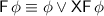
In a different research thread [15], the authors introduce the notion of monitorable specifications that can be positively or negatively determined by a finite trace. The monitorability of LTL is further studied in [6, 14]. This classification of specifications is orthogonal to our work. We focus on providing a sensible evaluation to all LTL properties, including the non-monitorable ones (e.g., ).

We also mention the recent work on statistical model checking for LTL [8]. In this work, the authors assume a gray-box setting, where the system-under-test (SUT) is a Markov chain with the known minimum transition probability. This is in contrast to our work, in which we passively observe existing finite traces generated by the SUT, i.e., we have a blackbox setting.

In [1], the authors propose extending LTL with a discounting operator and study the properties of the augmented logic. The LTL specification formalism is extended with path-accumulation assertions in [7]. These LTL extensions are motivated by the need for a more quantitative and refined analysis of the systems. In our work, the motivation for the counting semantics is quite different. We use the quantitative information that we collect during the execution of the trace to predict the future behavior of the system and thus improve the quality of the monitoring verdict.

3 Preliminaries

We first introduce traces and Linear Temporal Logic (LTL) that we interpret over 3-valued semantics.

Definition 1

(Trace). Let P a finite set of propositions and let $\varPi =2^P$. A (finite or infinite) trace $\pi$ is a sequence $\pi _{1}, \pi _{2}, \ldots \in \varPi ^* \cup \varPi ^\omega$ . We denote by $|\pi | \in \mathbb {N} \cup \{ \infty \}$ the length of $\pi$. We denote by $\pi \cdot \pi '$ the concatenation of $\pi \in \varPi ^*$ and $\pi ' \in \varPi ^* \cup \varPi ^\omega$.

Definition 2

(Linear Temporal Logic). In this paper, we consider linear temporal logic (LTL) and we define its syntax by the grammar:

where $p \in P$. We denote by $\varPhi$ the set of all LTL formulas.

From the basic definition we can derive other standard Boolean and temporal operators as follows:

Let $\pi \in \varPi ^{\omega }$ be an infinite trace and $\phi$ an LTL formula. The satisfaction relation $(\pi , i) \models \phi$ is defined inductively as follows

We now recall the 3-valued semantics from [4]. We denote by $[\pi \models _{3} \phi ]$ the evaluation of $\phi$ with respect to the trace $\pi \in \varPi ^{*}$ that yields a value in $\{ \top , \bot , {?}\}$.

$$\begin{array}{lll} [\pi \models _{3} \phi ]&{} = &{} \begin{aligned} {\left\{ \begin{array}{ll} \top &{} \forall \pi ' \in \varPi ^{\omega }, \pi \cdot \pi ' \models \phi \text {,} \\ \bot &{} \forall \pi ' \in \varPi ^{\omega }, \pi \cdot \pi ' \not \models \phi \text {,} \\ {?}&{} \text {otherwise}. \\ \end{array}\right. } \end{aligned}\\ \end{array}$$

We now restrict LTL to a fragment without explicit $\top$ and $\bot$ symbols and with the explicit operator that we add to the syntax. We provide an alternative 3-valued semantics for this fragment, denoted by $\mu _\pi (\phi , i)$ where $i \in \mathbb {N}_{>0}$ indicates a position in or outside the trace. We assume the order $\bot< ? < \top$, and extend the Boolean operations to the 3-valued domain with the rules $\lnot _3 \top = \bot$, $\lnot _3 \bot = \top$ and $\lnot _3 ? = ?$ and $\phi _1 \vee _3 \phi _2 = max(\phi _1,\phi _2)$. We define the semantics inductively as follows:

We note that the adapted semantics allows evaluating a finite trace in polynomial time, in contrast to $[\pi \models _{3} \phi ]$, which requires a $\textsc {PSPACE}$-complete algorithm. This improvement in complexity comes at a price – the adapted semantics cannot semantically characterize tautologies and contradiction. We have for example that $\mu _\pi (p \vee \lnot p, 1)$ for the empty word evaluates to ${?}$, despite the fact that $p \vee \lnot p$ is semantically equivalent to $\top$. The novel semantics that we introduce in the following sections make the same tradeoff.

In the following lemma, we relate the two three-valued semantics.

Lemma 3

Given an LTL formula and a trace $\pi \in \varPi ^{*}$, $|\pi | \ne 0$, we have that

$$ \begin{array}{lll} \mu _\pi (\phi ,1) = \top &{} \Rightarrow &{} [\pi \models _{3} \phi ] = \top \text {,}\\ \mu _\pi (\phi ,1) = \bot &{} \Rightarrow &{} [\pi \models _{3} \phi ] = \bot \text {.}\\ \end{array} $$

Proof

These two statements can be proven by induction on the structure of the LTL formula (see Appendix A.1 in [2]). $[\pi \models _{3} \phi ] = \; {?}\Rightarrow \mu _\pi (\phi ,1) = \; {?}$ is the consequence of the first two.

4 Counting Finitary Semantics for LTL

In this section, we introduce the counting semantics for LTL. We first provide necessary definitions in Sect. 4.1, we present the new semantics in Sect. 4.2 and finally propose a predictive mapping that transforms the counting semantics into a qualitative 5-valued verdict in Sect. 4.3.

4.1 Definitions

Let $\mathbb {N}_{+} = \mathbb {N}_0 \cup \{ \infty , -\}$ be the set of natural numbers (incl. 0) extended with the two special symbols $\infty$ ($\mathsf {infinite}$) and $-$ ($\mathsf {impossible}$) such that $\forall n \in \mathbb {N}_0$, we define $n< \infty < -$. We define the addition $\oplus$ of two elements $a,b \in \mathbb {N}_{+}$ as follows.

Definition 4

(Operator $\oplus$). We define the binary operator $\oplus : \mathbb {N}_{+} \times \mathbb {N}_{+} \rightarrow \mathbb {N}_{+}$ s. t. for $a \oplus b$ with $a, b \in \mathbb {N}_{+}$ we have $a + b$ if $a,b \in \mathbb {N}_0$ and $\max \{ a,b \}$ otherwise.

We denote by (s, f) a pair of two extended numbers $s,f \in \mathbb {N}_{+}$. In Definition 5, we introduce several operations on pairs: (1) the swap between the two values ($\sim$), (2) the increment by 1 of both values ($\oplus 1$), (3) the minmax binary operation ($\sqcup$) that gives the pair consisting of the minimum first value and the maximum second value, and (4) the maxmin binary operation ($\sqcap$) that is symmetric to ($\sqcup$).

Definition 7 introduces the counting semantics for LTL that for a finite trace $\pi$ and LTL formula $\phi$ gives a pair $(s,f) \in \mathbb {N}_{+} \times \mathbb {N}_{+}$. We call s and f satisfaction and violation witness counts, respectively. Intuitively, the s (f) value denotes the minimal number of additional steps that is needed to witness the satisfaction (violation) of the formula. The value $\infty$ is used to denote that the property can be satisfied (violated) only in an infinite number of steps, while $-$ means the property cannot be satisfied (violated) by any continuation of the trace.

Definition 5

(Operations $\sim$, $\oplus 1$, $\sqcup$, $\sqcap$).

Given two pairs $(s,f) \in \mathbb {N}_+ \times \mathbb {N}_+$ and $(s',f')\in \mathbb {N}_+ \times \mathbb {N}_+$, we have:

$$\begin{array}{rcl} \sim (s,f) &{} = &{} (f,s)\text {,} \\ (s,f) \oplus 1&{} = &{} (s \oplus 1,f \oplus 1) \text {,}\\ (s,f) \sqcup (s',f') &{} = &{} (\min (s,s'), \max (f,f')) \text {,}\\ (s,f) \sqcap (s',f')&{} = &{} (\max (s,s'), \min (f,f')) \text {.} \\ \end{array}$$

Example 6

Given the pairs (0, 0), $(\infty ,1)$ and $(7,-)$ we have the following:

$$ \begin{array}{rclrcl} \sim (0,0) &{} = &{} (0,0)\text {,} \;\;\;\;&{} \sim (\infty ,1) &{} = &{} (1,\infty )\text {,} \\ (0,0) \oplus 1&{} = &{} (1,1) \text {,} \;\;\;\;&{} (\infty ,1) \oplus 1&{} = &{} (\infty ,2) \text {,} \\ (0,0) \sqcup (\infty ,1) &{} = &{} (0,1)\text {,}\;\; \;\;&{} (\infty ,1) \sqcup (7,-) &{} = &{} (7,-)\text {,} \\ (0,0) \sqcap (\infty ,1) &{} = &{} (\infty ,0)\text {,} \;\;\;\;&{} (\infty ,1) \sqcap (7,-) &{} = &{} (\infty ,1)\text {.} \\ \end{array} $$

Remark. Note that $\mathbb {N}_+ \times \mathbb {N}_+$ forms a lattice where $(s,f) \unlhd (s',f')$ when $s \ge s'$ and $f \le f'$ with join $\sqcup$ and meet $\sqcap$. Intuitively, larger values are closer to true.

4.2 Semantics

We now present our finitary semantics.

Definition 7

(Counting finitary semantics). Let $\pi \in \varPi ^{*}$ be a finite trace, $i \in \mathbb {N}_{>0}$ be a position in or outside the trace and $\phi \in \varPhi$ be an LTL formula. We define the counting finitary semantics of LTL as the function

$d_\pi ~:~\varPhi \times \varPi ^{*} \times \mathbb {N}_{>0}\rightarrow \mathbb {N}_{+} \times \mathbb {N}_{+}$ such that:

We now provide some motivations behind the above definitions.

• Proposition. A proposition is either evaluated before or after the end of the trace. If it is evaluated before the end of the trace and the proposition holds, the satisfaction and violations witness counts are trivially 0 and $-$, respectively. In the case that the proposition does not hold, we have the symmetric witness counts. Finally, we take an optimistic view in case of evaluating a proposition after the end of the trace: The trace can be extended to a trace with i steps s.t. either p holds or p does not hold.

• Negation. Negating a formula simply swaps the witness counts. If we witness the satisfaction of $\phi$ in n steps, we witness the violation of $\lnot \phi$ in n steps, and vice versa.

• Disjunction. We take the shorter satisfaction witness count, because the satisfaction of one subformula is enough to satisfy the property. And we take the longer violation witness count, because both subformulas need to be violated to violate the property.

• Next. The next operator naturally increases the witness counts by one step.

• Eventually. We use the rewriting rule to define the semantics of the eventually operator. When evaluating the formula after the end of the trace, we replace the remaining obligation () by $(-,\infty )$. Thus, evaluated on the empty word is satisfied by a suffix that satisfies $\phi$, and it is violated only by infinite suffixes.

• Until. We use the same principle for defining the until semantics that we used for the eventually operator. We use the rewriting rule . On the empty word, is satisfied (in the shortest way) by a suffix that satisfies $\psi$, and it is violated by a suffix that violates both $\phi$ and $\psi$.

Example 8

We refer to our motivating example from Table 1 and evaluate the trace $\tau _{2}$ with respect to the specification $\psi$. We present the outcome in Table 2. We see that every proposition evaluates to $(0,-)$ when true. The satisfaction of a proposition that holds at time i is immediately witnessed and it cannot be violated by any suffix. Similarly, a proposition evaluates to $(-,0)$ when false. The valuations of count the number of steps to positions in which g holds. For instance, the first time at which g holds is $i=3$, hence evaluates to $(2,-)$ at time 1, $(1,-)$ at time 2 and $(0,-)$ at time 3. We also note that evaluates to $(0,\infty )$ at the end of the trace – it could be immediately satisfied with the continuation of the trace with g that holds, but could be violated only by an infinite suffix in which g never holds. We finally observe that evaluates to $(\infty ,\infty )$ at all positions – the property can be both satisfied and violated only with infinite suffixes.

Table 2. Unbounded response property example: $d_\pi (\phi , i)$ with the trace $\pi = \tau _{2}$.

Not all pairs $(s,f) \in \mathbb {N}_{+} \times \mathbb {N}_{+}$ are possible according to the counting semantics. We present the possible pairs in Lemma 9.

Lemma 9

Let $\pi \in \varPi ^{*}$ be a finite trace, $\phi$ an LTL formula and $i\in \mathbb {N}_0$ an index. We have that $d_\pi (\phi ,i)$ is of the form $(a,-)$, $(-,a)$, $(b_{1}, b_{2})$, $(b_{1},\infty )$, $(\infty , b_{2})$ or $(\infty , \infty )$, where $a \le |\pi | - i$ and $b_{j} > |\pi | - i$ for $j \in \{1,2\}$.

Proof

The proof can be obtained using structural induction on the LTL formula (see Appendix A.2 in [2]).

Finally, we relate our counting semantics to the three valued semantics in Lemma 10.

Lemma 10

Given an LTL formula and a trace $\pi \in \varPi ^{*}$ where $i \in \mathbb {N}_{>0}$ is an index and $\phi$ is an LTL formula, we have that

where $a \le |\pi | - i$ and $b_{j}$ is either $\infty$ or $b_{j} > |\pi | - i$ for $j \in \{1,2\}$.

Intuitively, Lemma 10 holds because we only introduce the symbol “$-$” within the trace when a satisfaction (violation) is observed. And the values of a pair only propagate into the past (and never into the future).

4.3 Evaluation

We now propose a mapping that predicts a qualitative verdict from our counting semantics. We adopt a 5-valued set consisting of $\mathsf {true}$ ($\top$), presumably true ($\top \!_P$), $\mathsf {inconclusive}$ (${?}$), presumably false ($\bot _P$) and $\mathsf {false}$ ($\bot$) verdicts. We define the following order over these five values: $\bot< \bot _P< {?}< \top \!_P< \top$. We equip this 5-valued domain with the negation ($\lnot$) and disjunction ($\vee$) operations, letting $\lnot \top = \bot$, $\lnot \top \!_P= \bot _P$, $\lnot {?}= {?}$, $\lnot \bot _P= \top \!_P$, $\lnot \bot = \top$ and $\phi _{1} \vee \phi _{2} = \max \{ \phi _{1}, \phi _{2} \}$. We define other Boolean operators such as conjunction by the usual logical equivalences ($\phi _{1} \wedge \phi _{2} = \lnot (\lnot \phi _{1} \vee \lnot \phi _{2})$, etc.).

We evaluate a property on a trace to $\top$ ($\bot$) when the satisfaction (violation) can be fully determined from the trace, following the definition of the three-valued semantics $\mu$. Intuitively, this takes care of the case in which the safety (co-safety) part of a formula has been violated (satisfied), at least for properties that are intentionally safe (intentionally co-safe, resp.) [10].

Whenever the truth value is not determined, we distinguish whether $d_\pi (\phi ,i)$ indicates the possibility for a satisfaction, respective violation, in finite time or not. For possible satisfactions, respective violations, in finite time we make a prediction on whether past observations support the believe that the trace is going to satisfy or violate the property. If the predictions are not inconclusive and not contradicting, then we evaluate the trace to the (presumable) truth value $\top \!_P$ or$\bot _P$. If we cannot make a prediction to a truth value, we compute the truth value recursively based on the operator in the formula and the truth values of the subformulas (with temporal operators unrolled).

We use the predicate $\text {pred}_\pi$ to give the prediction based on the observed witnesses for satisfaction. The predicate $\text {pred}_\pi (\phi ,i)$ becomes ${?}$ when no witness for satisfaction exists in the past. When there exists a witness that requires at least the same amount of additional steps as the trace under evaluation then the predicate evaluates to $\top$. If all the existing witnesses (and at least one exists) are shorter than the current trace, then the predicate evaluates to $\bot$. For a prediction on the violation we make a prediction on the satisfaction of $d_\pi (\lnot \phi ,i)$, i.e., we compute $\text {pred}_\pi (\lnot \phi ,i)$.

Definition 11

(Prediction predicate). Let s, f denote natural numbers and let $s_\pi (\phi ,i), f_\pi (\phi ,i) \in \mathbb {N}_+$ such that $d_\pi (\phi ,i)=\big (s_\pi (\phi ,i),f_\pi (\phi ,i) \big )$. We define the 3-valued predicate $\text {pred}_\pi$ as

For the evaluation we consider a case split among the possible combinations of values in the pairs.

Definition 12

(Predictive evaluation). We define the predictive evaluation function $e_\pi (\phi ,i)$, with $a \le |\pi | - i$ and $b_{j} > |\pi | - i$ for $j \in \{1,2\}$ and $a,b_j \in \mathbb {N}_0$, for the different cases of $d_\pi (\phi ,i)$:

where $r_\pi (\phi ,i)$ is an auxiliary function defined inductively as follows:

The predictive evaluation function is symmetric. Hence, $e_\pi (\phi ,i) = \lnot e_\pi (\lnot \phi ,i)$ holds.

Example 13

The outcome of evaluating $\tau _2$ from Table 1 is shown in Table 3. Subformula is predicted to be $\top \!_P$ at $i=7$ because there exists a longer witness for satisfaction in the past (e.g., at $i=1$). Thus, the trace evaluates to $\top \!_P$, as expected.

Table 3. Unbounded response property example with $\pi = \tau _{2}$.

Fig. 1.

Lattice for (s, f) with $\phi$ and $i < |\pi |$ fixed.

In Fig. 1 we visualize the evaluation of a pair $d_\pi (\phi ,i) = (s,f)$ for a fixed $\phi$ and a fixed position i. On the x-axis is the witness count s for a satisfaction and on the y-axis is the witness count f for a violation. For a value s, respectively f, that is smaller than the length of the suffix starting at position i (with the other value of the pair always being $-$), the evaluation is either $\top$ or $\bot$. Otherwise the evaluation depends on the values $s_{max}$ and $f_{max}$. These two values represent the largest witness counts for a satisfaction and a violation in the past, i.e., for positions smaller than i in the trace. Based on the prediction function $\text {pred}_\pi (\phi ,i)$ the evaluation becomes $\top _P$, ${?}$ or $\bot _P$, where ${?}$ indicates that the auxiliary function $r_\pi (\phi ,i)$ has to be applied. Starting at an arbitrary point in the diagram and moving to the right increases the witness count for a satisfaction while the witness count for a violation remains constant. Thus, moving to the right makes the pair “more false”. The same holds when keeping the witness count for a satisfaction constant and moving up in the diagram as this decrease the witness count for a violation. Analogously, moving down and/or left makes the pair “more true” as the witness count for a violation gets larger and/or the witness count for a satisfaction gets smaller.

Our 5-valued predictive evaluation refines the 3-valued LTL semantics.

Theorem 14

Let $\phi$ be an LTL formula, $\pi \in \varPi ^{*}$ and $i \in \mathbb {N}_{>0}$. We have

$$ \begin{array}{lllll} \mu _\pi (\phi ,i) = &{} \top &{} \leftrightarrow &{} e_\pi (\phi , i) = &{} \top \text {,}\\ \mu _\pi (\phi ,i) = &{} \bot &{} \leftrightarrow &{} e_\pi (\phi , i) = &{} \bot \text {,}\\ \mu _\pi (\phi ,i) = &{} {?}&{} \leftrightarrow &{} e_\pi (\phi , i) \in &{} \{ \top \!_P, \bot _P, {?}\} \text {.}\\ \end{array} $$

Theorem 14 holds, because the evaluation to $\top$ and $\bot$ is simply the mapping of a pair that contains the symbol “$-$”, which we have shown in Lemma 10.

Remember that $\mathbb {N}_+ \times \mathbb {N}_+$ is partially ordered by $\unlhd$. We now show that having a trace that is “more true” than another is correctly reflected in our finitary semantics. To define “more true”, we first need the polarity of a proposition in an LTL formula.

Example 15

Note that g has positive polarity in . If we define $\tau '_2$ to be as $\tau _2$, except that $g \in \tau '_2(i)$ for $i \in \{1,\dots ,6\}$, we have $e_{\tau '_2}(\phi ,i) = \bot _P$, whereas $e_{\tau _2}(\phi ,i) = \top \!_P$.

Definition 16

(Polarity). Let $\# \lnot$ be the number of negation operators on a specific path in the parse tree of $\phi$ starting at the root. We define the polarity as the function $\text {pol}(p)$ with proposition p in an LTL formula $\phi$ as follows:

$$\begin{aligned} \text {pol}(p) = {\left\{ \begin{array}{ll} \text {pos,} &{} \text {if } \# \lnot \text { on all paths to a leaf with proposition } p \text { is even,}\\ \text {neg,} &{} \text {if } \# \lnot \text { on all paths to a leaf with proposition } p \text { is odd,}\\ \text {mixed, }&{} \text {otherwise.}\\ \end{array}\right. } \end{aligned}$$

With the polarity defined, we now define the constraints for a trace to be “more true” with respect to an LTL formula $\phi$.

Definition 17

($\pi \sqsubseteq _\phi \pi '$). Given two traces $\pi$ and $\pi '$ of equal length and an LTL formula $\phi$ over proposition p, we define that $\pi \sqsubseteq _\phi \pi '$ iff

Whenever one trace is “more true” than another, this is correctly reflected in our finitary semantics.

Theorem 18

For two traces $\pi$ and $\pi '$ of equal length and an LTL formula $\phi$ over proposition p, we have that

$$ \pi \sqsubseteq _\phi \pi ' \Rightarrow d_{\pi '}(\phi ,1) \unlhd d_{\pi }(\phi ,1). $$

Therefore, we have for $\pi \sqsubseteq _\phi \pi '$ that

$$\begin{aligned} e_{\pi }(\phi , 1) = \top \Rightarrow e_{\pi '}(\phi , 1) = \top&\text {, and}\\ e_{\pi }(\phi , 1) = \bot \Leftarrow e_{\pi '}(\phi , 1) = \bot&. \end{aligned}$$

Theorem 18 holds, because we have that replacing an arbitrary observed value in $\pi$ by one with positive polarity in $\pi '$ always results with $d_{\pi }(\phi ,1)=(s,f)$ and $d_{\pi '}(\phi ,1)=(s',f')$ in $s' \le s$ and $f' \ge f$, as with $\pi \sqsubseteq _\phi \pi '$ we have that $\pi '$ witnesses a satisfaction of $\phi$ not later than $\pi$ and $\pi '$ also witness a violation of $\phi$ not earlier than $\pi$.

Table 4. Making a system “more true”.

Table 5. Examples of LTL specifications and traces

In Table 4 we give examples to illustrate the transition of one evaluation to another one. Note that it is possible to change from $\top \!_P$ to $\bot _P$. However, this is only the predicated truth value that becomes “worse”, because we have strengthened the prefix on which the prediction is based on, the values of $d_\pi (\phi ,i)$ do not change and remain the same is such a case.

5 Examples

We demonstrate the strengths and weaknesses of our approach on the examples of LTL specifications and traces shown in Table 5. We fully develop these examples in Appendix B in [2].

Table 6 summarizes the evaluation of our examples. The first and the second column denote the evaluated specification and trace. We use these examples to compare LTL with counting semantics (c-LTL) presented in this paper, to the other two popular finitary LTL interpretations, the 3-valued LTL semantics [4] (3-LTL) and LTL on trucated paths [9] (t-LTL). We recall that in t-LTL there is a distinction between a weak and a strong next operator. We denote by t-LTL-s (t-LTL-w) the specifications from our examples in which is interpreted as the strong (weak) next operator and assume that we always give a strong interpretation to and and a weak interpretation to .

Table 6. Comparison of different verdicts with different semantics

There are two immediate observations that we can make regarding the results presented in Table 6. First, the 3-valued LTL gives for all the examples an inconclusive verdict, a feedback that after all has little value to a verification engineer. The second observation is that the verdicts from c-LTL and t-LTL can differ quite a lot, which is not very surprising given the different strategies to interpret the unseen future. We now further comment on these examples, explaining in more details the results and highlighting the intuitive outcomes of c-LTL for a large class of interesting LTL specifications.

Effect of Nested Next. We evaluate with $\psi _{1}$ and $\psi _{2}$ the effect of nesting in an and an formula, respectively. We make a prediction on at the end of the trace before evaluating and . As a consequence, we find that $(\psi _{1}, \pi _{1})$ evaluates to presumably false, while $(\psi _{2}, \pi _{2})$ evaluates to presumably true. In t-LTL, this class of specification is very sensitive to the weak/strong interpretation of next, as we can see from the verdicts.

Request/Grants. We evaluate the request/grant property $\psi _{3}$ from the motivating example on the trace $\pi _{3}$. We observe that r at cycle 2 is followed by g at cycle 3, while r at cycle 5 is not followed by g at cycle 6. Hence, $(\psi _{3}, \pi _{3})$ evaluates to presumably false.

Concurrent Request/Grants. We evaluate the specification $\psi _{4}$ against the trace $\pi _{4}$. In this example $r_{1}$ is triggered at even time stamps and $r_{2}$ is triggered at odd time stamps. Every request is granted in one cycle. It follows that regardless of the time when the trace ends, there is one request that is not granted yet. We note that $\psi _{4}$ is a conjunction of two basic request/grant properties and we make independent predictions for each conjunct. Every basic request/grant property is evaluated to presumably true, hence $(\psi _{4}, \pi _{4})$ evaluates to presumably true. At this point, we note that in t-LTL, every request that is not granted by the end of the trace results in the property violation, regardless of the past observations.

Until. We use the specification $\psi _{5}$ and the trace $\pi _{5}$ to evaluate the effect of on the predictions. The specification requires that continuously holds until becomes true. We can see that in $\pi _{5}$ is witnessed at cycles $1-4$, while is witnessed at cycle 5. We can also see that is again witnessed from cycle 6 until the end of the trace at cycle 8. As a consequence, $(\psi _{5}, \pi _{5})$ is evaluated to presumably true.

Stabilization. The specification $\psi _{6}$ says that the value of g has to eventually stabilize to either true or false. We evaluate the formula on two traces $\pi _{6}$ and $\pi _{7}$. In the trace $\pi _{6}$, g alternates between true and false every two cycles and becomes true in the last cycle. Hence, there is no sufficiently long witness of trace stabilization $(\psi _{6}, \pi _{6})$ evaluates to presumably false. In the trace $\pi _{7}$, g also alternates between true and false every two cycles, but in the last four cycles g remains continuously true. As a consequence, $(\psi _{6}, \pi _{7})$ evaluates to presumably true. This example also illustrates the importance of when the trace truncation occurs. If both $\pi _{6}$ and $\pi _{7}$ were truncated at cycle 5, both $(\psi _{6}, \pi _{6})$ and $(\psi _{6}, \pi _{7})$ would evaluate to presumably false. We note that $\psi _{6}$ is satisfied by all traces in t-LTL.

Sub-formula Domination. The specification $\psi _{7}$ exposes a weakness of our approach. It requires that in every cycle, either r or g is witnessed in some unbounded future. With our approach, $(\psi _{7}, \pi _{8})$ evaluates to presumably false. This is against our intuition because we have observed that g becomes regularly true very second time step. However, in this example our prediction for dominates over the prediction for , leading to the unexpected presumably false verdict. On the other hand, t-LTL interpretation of the same specification is dependent only on the last value of r and g.

Semantically Equivalent Formulas. We now demonstrate that our approach may give different answers for semantically equivalent formulas. For instance, both $\psi _{8}$ and $\psi _{9}$ are semantically equivalent to $\psi _{7}$. We have that $(\psi _{8}, \pi _{8})$ evaluates to presumably false, while $(\psi _{9}, \pi _{8})$ evaluates to presumably true. We note that t-LTL verdicts are stable for semantically different formulas.

6 Conclusion

We have presented a novel finitary semantics for LTL that uses the history of satisfaction and violation in a finite trace to predict whether the co-safety and safety aspects of a formula will be satisfied in the extension of the trace to an infinite one. We claim that the semantics closely follow human intuition when predicting the truth value of a trace. The presented examples (incl. non-monitorable LTL properties) illustrate our approach and support this claim.

Our definition of the semantics is trace-based, but it is easily extended to take an entire database of traces into account, which may make the approach more precise. Our approach currently uses a very simple form of learning to predict the future. We would like to consider more sophisticated statistical methods to make better predictions. In particular, we plan to apply nonparametric statistical methods (i.e., the Wilcoxon signed-rank test [16]), in combination with our counting semantics, to identify and quantify the traces that are outliers.

References

Almagor, S., Boker, U., Kupferman, O.: Discounting in LTL. In: Ábrahám, E., Havelund, K. (eds.) TACAS 2014. LNCS, vol. 8413, pp. 424–439. Springer, Heidelberg (2014). https://doi.org/10.1007/978-3-642-54862-8_37
Bartocci, E., Bloem, R., Nickovic, D., Roeck, F.: A counting semantics for monitoring LTL specifications over finite traces. CoRR, abs/1804.03237 (2018)
Bartocci, E., Falcone, Y. (eds.): Lectures on Runtime Verification. LNCS, vol. 10457. Springer, Cham (2018). https://doi.org/10.1007/978-3-319-75632-5
Bauer, A., Leucker, M., Schallhart, C.: Monitoring of real-time properties. In: Arun-Kumar, S., Garg, N. (eds.) FSTTCS 2006. LNCS, vol. 4337, pp. 260–272. Springer, Heidelberg (2006). https://doi.org/10.1007/11944836_25
Bauer, A., Leucker, M., Schallhart, C.: The good, the bad, and the ugly, but how ugly is ugly? In: Sokolsky, O., Taşıran, S. (eds.) RV 2007. LNCS, vol. 4839, pp. 126–138. Springer, Heidelberg (2007). https://doi.org/10.1007/978-3-540-77395-5_11
Bauer, A., Leucker, M., Schallhart, C.: Runtime verification for LTL and TLTL. ACM Trans. Softw. Eng. Methodol. 20(4), 14:1–14:64 (2011)
Boker, U., Chatterjee, K., Henzinger, T.A., Kupferman, O.: Temporal specifications with accumulative values. ACM Trans. Comput. Logic 15(4), 27:1–27:25 (2014)
Daca, P., Henzinger, T.A., Křetínský, J., Petrov, T.: Faster statistical model checking for unbounded temporal properties. In: Chechik, M., Raskin, J.-F. (eds.) TACAS 2016. LNCS, vol. 9636, pp. 112–129. Springer, Heidelberg (2016). https://doi.org/10.1007/978-3-662-49674-9_7
Eisner, C., Fisman, D., Havlicek, J., Lustig, Y., McIsaac, A., Van Campenhout, D.: Reasoning with temporal logic on truncated paths. In: Hunt, W.A., Somenzi, F. (eds.) CAV 2003. LNCS, vol. 2725, pp. 27–39. Springer, Heidelberg (2003). https://doi.org/10.1007/978-3-540-45069-6_3
Kupferman, O., Vardi, M.Y.: Model checking of safety properties. Form. Methods Syst. Des. 19(3), 291–314 (2001)
Manna, Z., Pnueli, A.: The Temporal Logic of Reactive and Concurrent Systems - Specification. Springer, Heidelberg (1992). https://doi.org/10.1007/978-1-4612-0931-7
Morgenstern, A., Gesell, M., Schneider, K.: An asymptotically correct finite path semantics for LTL. In: Bjørner, N., Voronkov, A. (eds.) LPAR 2012. LNCS, vol. 7180, pp. 304–319. Springer, Heidelberg (2012). https://doi.org/10.1007/978-3-642-28717-6_24
Pnueli, A.: The temporal logic of programs. In: 18th Annual Symposium on Foundations of Computer Science, Providence, Rhode Island, USA, 31 October–1 November 1977, pp. 46–57 (1977)
Pnueli, A., Zaks, A.: PSL model checking and run-time verification via testers. In: Misra, J., Nipkow, T., Sekerinski, E. (eds.) FM 2006. LNCS, vol. 4085, pp. 573–586. Springer, Heidelberg (2006). https://doi.org/10.1007/11813040_38
Viswanathan, M., Kim, M.: Foundations for the run-time monitoring of reactive systems – fundamentals of the MaC language. In: Liu, Z., Araki, K. (eds.) ICTAC 2004. LNCS, vol. 3407, pp. 543–556. Springer, Heidelberg (2005). https://doi.org/10.1007/978-3-540-31862-0_38
Wilcoxon, F.: Individual comparisons by ranking methods. Biom. Bull. 1(6), 80–83 (1945)
Zhang, X., Leucker, M., Dong, W.: Runtime verification with predictive semantics. In: Goodloe, A.E., Person, S. (eds.) NFM 2012. LNCS, vol. 7226, pp. 418–432. Springer, Heidelberg (2012). https://doi.org/10.1007/978-3-642-28891-3_37
Author information
Authors and Affiliations
Corresponding author
Editor information
Editors and Affiliations
Rights and permissions
<SimplePara><Emphasis Type="Bold">Open Access</Emphasis>This chapter is licensed under the terms of the Creative Commons Attribution 4.0 International License(http://creativecommons.org/licenses/by/4.0/), which permits use, sharing, adaptation, distribution and reproduction in any medium or format, as long as you give appropriate credit to the original author(s) and the source, provide a link to the Creative Commons license and indicate if changes were made.</SimplePara><SimplePara>The images or other third party material in this chapter are included in the chapter's Creative Commons license, unless indicated otherwise in a credit line to the material. If material is not included in the chapter's Creative Commons license and your intended use is not permitted by statutory regulation or exceeds the permitted use, you will need to obtain permission directly from the copyright holder.</SimplePara>
Copyright information
© 2018 The Author(s)
About this paper
Cite this paper
Bartocci, E., Bloem, R., Nickovic, D., Roeck, F. (2018). A Counting Semantics for Monitoring LTL Specifications over Finite Traces. In: Chockler, H., Weissenbacher, G. (eds) Computer Aided Verification. CAV 2018. Lecture Notes in Computer Science(), vol 10981. Springer, Cham. https://doi.org/10.1007/978-3-319-96145-3_29
Download citation
DOI: https://doi.org/10.1007/978-3-319-96145-3_29
Published:
Publisher Name: Springer, Cham
Print ISBN: 978-3-319-96144-6
Online ISBN: 978-3-319-96145-3
eBook Packages: Computer ScienceComputer Science (R0)