Milling Dynamics

Abstract

This chapter describes regenerative chatter in milling. Similar to Chap. 3, both analytical and numerical analyses are presented to predict the process behavior. The analytical, frequency domain stability lobe diagram is adapted to milling. Two algorithms are described: average tooth angle and Fourier series. Time domain simulations for square (straight teeth and helical teeth) and ball endmills (helical teeth) are detailed. The cutting force model is then extended and an experimental procedure for identifying the cutting force coefficients is derived for two different fitting approaches. Finally, the effect of process damping on milling stability at low speeds is presented.

If we knew what it was we were doing, it would not be called research, would it?

—Albert Einstein

Appendices

Exercises

• 1. Compute the start and exit angles for the following milling cases.

  • (a) Up milling, 30% radial immersion

  • (b) Down milling, 40% radial immersion

• 2. Determine the tooth passing frequency for a cutter with three teeth rotating at 10,000 rpm.

• 3. Calculate the maximum y direction force for a 40% radial immersion down milling cut carried out using a three tooth end mill; see Fig. 4.82. The material-tool combination gives: k_t = 720 N/mm² and k_n = 200 N/mm² (aluminum alloy). Also, b = 2.5 mm and f_t = 0.2 mm/tooth. Assume a rigid cutting tool and workpiece.

• 4. For the average tooth angle milling stability analysis, complete parts (a) through (d). A 35% radial immersion up milling cut is to be performed using a square end mill with four teeth and the force angle, β, is 68 deg. See Fig. 4.83.

  • (a) Determine the average angle of a tooth in the cut.

  • (b) Calculate the directional orientation factors.

  • (c) Compute the oriented frequency response function and identify the valid chatter frequency range(s) in Hz. The x direction dynamics are given by: f_nx = 1000 Hz, k_x = 7 × 10⁶ N/m, and ζ_x = 0.03 and the y direction dynamics are: f_ny = 1200 Hz, k_y = 6 × 10⁷ N/m, and ζ_y = 0.04. You may assume that these single degree of freedom parameters were obtained from a modal fit to frequency responses measured in the x and y directions with bandwidths of 0–2500 Hz.

  • (d) Plot the first five stability lobes, N = 0 to 4. The workpiece material is 1020 carbon steel; see Table 3.1.

• 5. For the cut described in Exercise 4, use the Fourier approach to obtain the stability lobe diagram (j = 0 to 4).

• 6. Calculate the lowest axial depth for which a constant cutting force is obtained independent of the selected radial depth of cut. The helical square end mill has a diameter of 10 mm, six teeth, and a 42 deg helix angle.

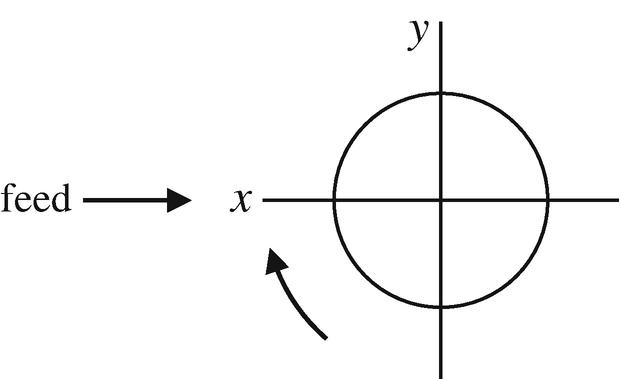
• 7. For a particular milling application, the spindle speed is 6000 rpm. The x and y direction cutting forces are shown in Fig. 4.84. The coordinate system is defined in Fig. 4.85. Only one tooth is engaged in the cut at any time and the cut is stable. The cutter teeth are straight.

  • (a) Is this cut up or down milling?

  • (b) How many teeth are on the milling cutter?

  • (c) If the Fourier transform for either cutting force signal (x or y direction) were computed, at what frequencies (in Hz) would peaks be expected?

  • (d) Determine k_t and k_n, where the tangential and normal force components are expressed as: F_t = k_tbh and F_n = k_nbh, where b = 5 mm, f_t = 0.2 mm/tooth, and the circular tool path approximation may be applied.

• 8. An endmill with four teeth is being used in a cut with an entry (starting) angle of 15 deg and an exit angle of 75 deg.

  • (a) Determine the average number of teeth in the cut (average tooth angle approach).

  • (b) What is the average angle of the surface normal for a tooth engaged in the cut (average tooth angle approach)? Sketch the cut and identify the surface normal and angle on your sketch.

    

  • (c) If β = 60 deg (average tooth angle approach), determine the directional orientation factors.

Fig. 4.82

Down milling force geometry

Fig. 4.83

35% radial immersion up milling geometry

Fig. 4.84

Time domain forces in the x and y directions

Fig. 4.85

Coordinate system for forces

Appendix: Reformulation of Fourier Series Eigenvalue Problem

In Sect. 4.3.3, we detailed the truncated Fourier series approach to obtaining the analytical stability limit for milling [5]. The dynamic milling equation (Eq. 4.49) was presented as:

$$ \left(\begin{array}{c}{F}_x\\ {}{F}_y\end{array}\right){\mathrm{e}}^{i{\omega}_{\mathrm{c}}t}=\frac{1}{2}{bK}_{\mathrm{t}}\left[{A}_0\right]\left(1-{\mathrm{e}}^{i{\omega}_{\mathrm{c}}\tau}\right)\left[\begin{array}{cc}{\mathrm{FRF}}_{xx}& 0\\ {}0& {\mathrm{FRF}}_{yy}\end{array}\right]\left(\begin{array}{c}{F}_x\\ {}{F}_y\end{array}\right){\mathrm{e}}^{i{\omega}_{\mathrm{c}}t}, $$

(4.117)

which is true if $\left(\begin{array}{c}{F}_x\\ {}{F}_y\end{array}\right){\mathrm{e}}^{i{\omega}_{\mathrm{c}}t}=\left[\begin{array}{cc}1& 0\\ {}0& 1\end{array}\right]\left(\begin{array}{c}{F}_x\\ {}{F}_y\end{array}\right){\mathrm{e}}^{i{\omega}_{\mathrm{c}}t}=\left[I\right]\left(\begin{array}{c}{F}_x\\ {}{F}_y\end{array}\right){\mathrm{e}}^{i{\omega}_{\mathrm{c}}t}$. This enables us to write $\frac{1}{2}{bK}_{\mathrm{t}}\left[{A}_0\right]\left(1-{\mathrm{e}}^{i{\omega}_{\mathrm{c}}\tau}\right)\left[\begin{array}{cc}{\mathrm{FRF}}_{xx}& 0\\ {}0& {\mathrm{FRF}}_{yy}\end{array}\right]=\left[I\right]$ or $\frac{N_{\mathrm{t}}}{4\pi }{bK}_{\mathrm{t}}\left(1-{\mathrm{e}}^{-i{\omega}_{\mathrm{c}}\tau}\right)\left[{\mathrm{FRF}}_{\mathrm{or}}\right]=\left[I\right]$. The eigenvalue problem was then posed in [5] as:

$$ \det \left(\left[I\right]+\Lambda \left[{\mathrm{FRF}}_{\mathrm{or}}\right]\right)=0, $$

(4.118)

where $\Lambda =-\frac{N_{\mathrm{t}}}{4\pi }{bK}_{\mathrm{t}}\left(1-{\mathrm{e}}^{-i{\omega}_{\mathrm{c}}\tau}\right)$ gives the eigenvalues. To apply the Matlab^® eig function, we must restate the eigenvalue problem as det([FRF_or] − λ[I]) = 0. The new complex eigenvalues are therefore $\lambda ={\lambda}_{\mathrm{Re}}+i{\lambda}_{\mathrm{Im}}=\frac{4\pi }{N_{\mathrm{t}}}\frac{1}{bK_{\mathrm{t}}\left(1-{\mathrm{e}}^{-i{\omega}_{\mathrm{c}}\tau}\right)}$. We determine the corresponding stability limit by solving this expression for b, rationalizing the result, and then substituting for ${\mathrm{e}}^{-i{\omega}_{\mathrm{c}}\tau }$ using the Euler identity ${\mathrm{e}}^{-i{\omega}_{\mathrm{c}}\tau }=\cos \left({\omega}_{\mathrm{c}}\tau \right)-i\sin \left({\omega}_{\mathrm{c}}\tau \right)$.

$$ {\displaystyle \begin{array}{l}{\tilde{b}}_{\mathrm{lim}}=\frac{4\pi }{N_{\mathrm{t}}{K}_{\mathrm{t}}\left({\lambda}_{\mathrm{Re}}+i{\lambda}_{\mathrm{Im}}\right)\left(1-{\mathrm{e}}^{-i{\omega}_{\mathrm{c}}\tau}\right)}\\ {}{\tilde{b}}_{\mathrm{lim}}=\frac{4\pi \left({\lambda}_{\mathrm{Re}}-i{\lambda}_{\mathrm{Im}}\right)}{N_{\mathrm{t}}{K}_{\mathrm{t}}\left({\lambda}_{\mathrm{Re}}+i{\lambda}_{\mathrm{Im}}\right)\left({\lambda}_{\mathrm{Re}}-i{\lambda}_{\mathrm{Im}}\right)\left(1-{\mathrm{e}}^{-i{\omega}_{\mathrm{c}}\tau}\right)}\\ {}{\tilde{b}}_{\mathrm{lim}}=\frac{4\pi \left({\lambda}_{\mathrm{Re}}-i{\lambda}_{\mathrm{Im}}\right)}{N_{\mathrm{t}}{K}_{\mathrm{t}}\left({\lambda_{\mathrm{Re}}}^2+{\lambda_{\mathrm{Im}}}^2\right)\left(1-\cos \left({\omega}_{\mathrm{c}}\tau \right)+i\sin \left({\omega}_{\mathrm{c}}\tau \right)\right)}\end{array}} $$

(4.119)

After the Euler identity substitution, we again rationalize to obtain Eq. 4.120.

$$ {\displaystyle \begin{array}{l}{\tilde{b}}_{\mathrm{lim}}=\frac{4\pi }{N_{\mathrm{t}}{K}_{\mathrm{t}}\left({\lambda_{\mathrm{Re}}}^2+{\lambda_{\mathrm{Im}}}^2\right)}\frac{\left({\lambda}_{\mathrm{Re}}-i{\lambda}_{\mathrm{Im}}\right)\left(1+\cos \left({\omega}_{\mathrm{c}}\tau \right)-i\sin \left({\omega}_{\mathrm{c}}\tau \right)\right)}{\left(1-\cos \left({\omega}_{\mathrm{c}}\tau \right)+i\sin \left({\omega}_{\mathrm{c}}\tau \right)\right)\left(1-\cos \left({\omega}_{\mathrm{c}}\tau \right)-i\sin \left({\omega}_{\mathrm{c}}\tau \right)\right)}\\ {}{\tilde{b}}_{\mathrm{lim}}=\frac{4\pi }{N_{\mathrm{t}}{K}_{\mathrm{t}}\left({\lambda_{\mathrm{Re}}}^2+{\lambda_{\mathrm{Im}}}^2\right)}\frac{\left({\lambda}_{\mathrm{Re}}-i{\lambda}_{\mathrm{Im}}\right)\left(1+\cos \left({\omega}_{\mathrm{c}}\tau \right)-i\sin \left({\omega}_{\mathrm{c}}\tau \right)\right)}{\left(2-2\cos \left({\omega}_{\mathrm{c}}\tau \right)\right)}\\ {}{\tilde{b}}_{\mathrm{lim}}=\frac{2\pi }{N_{\mathrm{t}}{K}_{\mathrm{t}}\left({\lambda_{\mathrm{Re}}}^2+{\lambda_{\mathrm{Im}}}^2\right)}\frac{\left(\begin{array}{l}\left({\lambda}_{\mathrm{Re}}\left(1-\cos \left({\omega}_{\mathrm{c}}\tau \right)\right)+{\lambda}_{\mathrm{Im}}\sin \left({\omega}_{\mathrm{c}}\tau \right)\right)\\ {}+i\left({\lambda}_{\mathrm{Im}}\left(1-\cos \left({\omega}_{\mathrm{c}}\tau \right)\right)-{\lambda}_{\mathrm{Re}}\sin \left({\omega}_{\mathrm{c}}\tau \right)\right)\end{array}\right)}{\left(1-\cos \left({\omega}_{\mathrm{c}}\tau \right)\right)}\end{array}} $$

(4.120)

Because ${\tilde{b}}_{\mathrm{lim}}$ must be real valued, the imaginary part from the parenthetical portion of the numerator in the final line in Eq. 4.120 must be equal to zero:

$$ {\lambda}_{\mathrm{Im}}\left(1-\cos \left({\omega}_{\mathrm{c}}\tau \right)\right)-{\lambda}_{\mathrm{Re}}\sin \left({\omega}_{\mathrm{c}}\tau \right)=0. $$

(4.121)

This gives $\frac{\lambda_{\mathrm{Im}}}{\lambda_{\mathrm{Re}}}=\frac{\sin \left({\omega}_{\mathrm{c}}\tau \right)}{1-\cos \left({\omega}_{\mathrm{c}}\tau \right)}=\tilde{\kappa}$. Substitution in Eq. 4.120 yields Eq. 4.122.

$$ {\displaystyle \begin{array}{l}{\tilde{b}}_{\mathrm{lim}}=\frac{2\pi }{N_{\mathrm{t}}{K}_{\mathrm{t}}\left({\lambda_{\mathrm{Re}}}^2+{\lambda_{\mathrm{Im}}}^2\right)}\left(\frac{\lambda_{\mathrm{Re}}\left(1-\cos \left({\omega}_{\mathrm{c}}\tau \right)\right)}{\left(1-\cos \left({\omega}_{\mathrm{c}}\tau \right)\right)}+\frac{\lambda_{\mathrm{Im}}\sin \left({\omega}_{\mathrm{c}}\tau \right)}{\left(1-\cos \left({\omega}_{\mathrm{c}}\tau \right)\right)}\right)\\ {}{\tilde{b}}_{\mathrm{lim}}=\frac{2\pi }{N_{\mathrm{t}}{K}_{\mathrm{t}}\left({\lambda_{\mathrm{Re}}}^2+{\lambda_{\mathrm{Im}}}^2\right)}\left({\lambda}_{\mathrm{Re}}+{\lambda}_{\mathrm{Im}}\tilde{\kappa}\right)\\ {}{\tilde{b}}_{\mathrm{lim}}=\frac{2\pi }{N_{\mathrm{t}}{K}_{\mathrm{t}}\left({\lambda_{\mathrm{Re}}}^2+{\lambda_{\mathrm{Im}}}^2\right)}{\lambda}_{\mathrm{Re}}\left(1+\frac{\lambda_{\mathrm{Im}}}{\lambda_{\mathrm{Re}}}\overset{\sim }{\kappa}\right)=\frac{2\pi }{N_{\mathrm{t}}{K}_{\mathrm{t}}\left({\lambda_{\mathrm{Re}}}^2+{\lambda_{\mathrm{Im}}}^2\right)}{\lambda}_{\mathrm{Re}}\left(1+{\overset{\sim }{\kappa}}^2\right)\end{array}} $$

(4.122)

References

Kumanchik, L., & Schmitz, T. (2007). Improved analytical chip thickness model for milling. Precision Engineering, 31, 317–324.
Tlusty, J., Zaton, W., & Ismail, F. (1983). Stability lobes in milling. Annals of the CIRP, 32(1), 309–313.
Smith, S., & Tlusty, J. (1990). Update on high-speed milling dynamics. Journal of Engineering for Industry, 112, 142–149.
Smith, S., & Tlusty, J. (1991). An overview of modeling and simulation of the milling process. Journal of Engineering for Industry, 113, 169–175.
Altintas, Y., & Budak, E. (1995). Analytical prediction of stability lobes in milling. Annals of the CIRP, 44(1), 357–362.
Davies, M., Pratt, J., Dutterer, B., & Burns, T. (2000). The stability of low radial immersion milling. Annals of the CIRP, 49(1), 37–40.
Davies, M., Pratt, J., Dutterer, B., & Burns, T. (2002). Stability prediction for low radial immersion milling. Journal of Manufacturing Science and Engineering, 124(2), 217–225.
Bayly, P., Mann, B., Schmitz, T., Peters, D., Stépàn, G., & Insperger, T. (2002). Effects of radial immersion and cutting direction on chatter instability in endmilling. In Proceedings of ASME International Mechanical Engineering Conference and Exposition, IMECE2002-34116, New Orleans, LA (on CD).
Mann, B., Bayly, P., Davies, M., & Halley, J. (2004). Limit cycles, bifurcations, and accuracy of the milling process. Journal of Sound and Vibration, 227, 31–48.
Schmitz, T., Davies, M., Medicus, K., & Snyder, J. (2001). Improving high-speed machining material removal rates by rapid dynamic analysis. Annals of the CIRP, 50(1), 263–268.
Schmitz, T., Medicus, K., & Dutterer, B. (2002). Exploring once-per-revolution audio signal variance as a chatter indicator. Machining Science and Technology, 6(2), 215–233.
Schmitz, T. (2003). Chatter recognition by a statistical evaluation of the synchronously sampled audio signal. Journal of Sound and Vibration, 262(3), 721–730.
Delio, T., Tlusty, J., & Smith, S. (1992). Use of audio signals for chatter detection and control. Journal of Engineering for Industry, 114, 146–157.
Honeycutt, A., & Schmitz, T. (2016). A new metric for automated stability identification in time domain milling simulation. Journal of Manufacturing Science and Engineering, 138(7), 074501.
Honeycutt, A., & Schmitz, T. (2017). Milling stability interrogation by subharmonic sampling. Journal of Manufacturing Science and Engineering, 139(4), 041009.
Tlusty, G. (2000). Manufacturing equipment and processes. Upper Saddle River, NJ: Prentice-Hall, Section 9.5.4.
Altintas, Y., & Lee, P. (1996). A general mechanics and dynamics model for helical end mills. Annals of the CIRP, 45(1), 59–64.
Altintas, Y. (2000). Manufacturing automation: metal cutting mechanics, machine tool vibrations, and CNC design. Cambridge: Cambridge University Press, Sect. 2.8.1.
Duncan, G. S. (2006). Milling dynamics prediction and uncertainty analysis using receptance coupling substructure analysis. Ph.D. Dissertation, University of Florida.
Koenisgberger, F., & Sabberwal, A. (1961). An investigation into the cutting force pulsations during milling operations. International Journal of Machine Tool Design and Research, 1, 15–33.
Tlusty, J., & MacNeil, P. (1975). Dynamics of cutting forces in end milling. Annals of the CIRP, 24(1), 21–25.
Kline, W., DeVor, R., & Lindberg, J. (1982). The prediction of cutting forces in end milling with applications to cornering cuts. International Journal of Machine Tool Design and Research, 22, 7–22.
Fu, H., DeVor, R., & Kapoor, S. (1984). A mechanistic model for the prediction of the force system in face milling operations. Journal of Engineering for Industry, 111, 27–36.
Yellowley, I. (1985). Observations of the mean values of forces, torque and specific power in the peripheral milling process. International Journal of Machine Tool Design and Research, 25, 337–346.
Amarego, E., & Whitfield, R. (1985). Computer based modeling of popular machining operations for forces and power prediction. Annals of the CIRP, 34, 65–69.
Wang, J.-J., Liang, S., & Book, W. (1994). Convolution analysis of cutting force pulsation. Journal of Engineering for Industry, 116, 17–25.
Endres, W., DeVor, R., & Kapoor, S. (1995). A dual-mechanism approach to the prediction of machining forces, Part 1: Model development. Journal of Engineering for Industry, 117, 526–533.
Budak, E., Altintas, Y., & Amarego, E. (1998). Prediction of milling force coefficients from orthogonal cutting data. Journal of Manufacturing Science and Engineering, 118, 216–224.
Jayaram, S., Kapoor, S., & DeVor, R. (2001). Estimation of the specific cutting pressures for mechanistic cutting force models. International Journal of Machine Tools and Manufacture, 41, 265–281.
Wang, J.-J., & Zheng, C. (2002). An analytical force model with shearing and ploughing mechanisms for end milling. International Journal of Machine Tools and Manufacture, 42, 761–771.
Chapra, S., & Canale, R. (1985). Numerical methods for engineers. New York, NY: McGraw-Hill Book Co., Section 10.1.
Rubeo, M., & Schmitz, T. (2016). Mechanistic force model coefficients: a comparison of linear regression and nonlinear optimization. Precision Engineering, 45, 311–321.
Coleman, T. F., & Li, Y. (1994). On the convergence of interior-reflective newton methods for nonlinear minimization subject to bounds. Mathematical Programming, 67, 189–224.
Smith, D., Smith, S., & Tlusty, J. (1998). High performance milling torque sensor. Journal of Manufacturing Science and Engineering, 120(3), 504–514.
Altintas, Y., Eynian, M., & Onozuka, H. (2008). Identification of dynamic cutting force coefficients and chatter stability with process damping. Annals of the CIRP, 57(1), 371–374.
Tyler, C., & Schmitz, T. (2012). Process damping analytical stability analysis and validation. Transactions of the NAMRI/SME, 40, 1–8.
Tyler, C., & Schmitz, T. (2013). Analytical process damping stability prediction. Journal of Manufacturing Processes, 15, 69–76.
Tyler, C., Karandikar, J., & Schmitz, T. (2013). Process damping coefficient identification using bayesian inference. Transactions of the NAMRI/SME, 41, 1–8.
Tyler, C., & Schmitz, T. (2014). Process damping milling model database. Transactions of the NAMRI/SME, 42, 1–8.
Tyler, C., Troutman, J., & Schmitz, T. (2015). Radial depth of cut stability lobe diagrams with process damping effects. Precision Engineering, 40, 318–324.
Tyler, C., Troutman, J., & Schmitz, T. (2016). A coupled dynamics, multiple degree of freedom process damping model, Part 1: Turning. Precision Engineering, 46, 65–72.
Tyler, C., Troutman, J., & Schmitz, T. (2016). A coupled dynamics, multiple degree of freedom process damping model, Part 2: Milling. Precision Engineering, 46, 73–80.
Author information
Authors and Affiliations