Almost Tight Multi-Instance Multi-Ciphertext Identity-Based Encryption on Lattices

Abstract

Boyen and Li [AsiaCrypt, 2016] proposed the first almost tightly secure lattice identity-based encryption scheme in the standard model. The security of such scheme is proved under learning with errors assumption in the single-instance, single-challenge setting. In this work, we show how to extend the Boyen-Li scheme to obtain an almost tight security reduction in the multi-instance, multi-ciphertext setting, in which the security loss incurred is $\textsf {poly}(\kappa )$ in the security parameter $\kappa$ and independent of the number of adversarial queries.

X. Boyen—Research supported in part by ARC Discovery Project grant number DP140103885 and ARC Future Fellowship FT140101145 from the Australian Research Council.

1 Introduction

To prove that the security of a cryptosystem is based on some computational problem, we provide a reductionist proof (in a properly defined security model) that states: If there exists an efficient adversary with runtime t that breaks the cryptosystem with non-negligible probability $\epsilon$, then an efficient algorithm can be constructed to solve the computational problem with non-negligible probability $\epsilon ' = \epsilon / L$ in time $t' \approx t$, which contradicts the assumed hardness of such computational problem. The parameter $L\ge 1$ measures the tightness of such a reduction proof. L usually can be affected by several factors, including the reductionist proof itself, the security parameter, the number of deployed instance of a cryptosystem, the number of adversarial queries and so on. We say a reductionist proof is tight if L is a small constant, and almost tight if L is a polynomial of the security parameter and independent of other factors. An (almost) tight reduction usually has smaller and fixed L, which allows us to implement the cryptosystem with shorter parameters in a more accurate way. In contrast, the parameter L in loose reductions is often large and depends on some uncontrollable quantities, e.g., the number of adversarial queries and the number of system instances. These quantities are difficult to determine accurately when the cryptosystem is deployed. Once these quantities are increased by adversaries, L could go beyond some bound fixed by the implementation, obscuring the cryptosystem’s security. Therefore, (almost) tight reduction is a desirable feature for cryptosystems.

In [11] the authors propose an almost tightly secure identity-based encryption (IBE) scheme from lattice. Its security is based on the hardness of learning-with-errors (LWE) problem and the security of an instantiated pseudorandom function (PRF). The reduction is tight in the sense that the security loss during the reduction is independent of the number of key generation queries, say $Q_{\textsf {key}}$, made by the adversary. To make the whole reduction tight, a PRF with tight reduction is required. However, the security reduction given by Boyen and Li [11] is within the “single instance, single challenge” (SISC) setting where the adversary is only given one instance of the IBE scheme and one challenge ciphertext to attack. In a more realistic scenario, many instances of an IBE scheme would be deployed and there would be many ciphertexts targeted by an adversary. To model this “multi-instance, multi-ciphertext” setting, the adversary is allowed to see any polynomial number of scheme instances, say N, adaptively make any polynomial number of identity key generation queries, say $Q_{\textsf {key}}$, and receive any polynomial number of challenge ciphertexts, say $Q_{\textsf {enc}}$. Generically, via a hybrid argument, if an IBE scheme $\varPi$ is $\epsilon$ secure (meaning that adversary breaks $\varPi$ with probability $\epsilon$ in a defined model) in the SISC setting, then $\varPi$ is $\epsilon ' = \epsilon \cdot N\cdot Q_{\textsf {enc}}$ secure in the MIMC setting. This security loss (i.e., $N\cdot Q_{\textsf {enc}}$) could be significant since N and $Q_{\textsf {enc}}$ are controlled by the adversary and, therefore, could be large. So it is preferable to have IBE schemes whose security does not depend on $Q_{\textsf {key}}$, $Q_{\textsf {enc}}$ and N in the MIMC setting.

The first construction of IBE schemes from bilinear pairings with tight reductions in the MIMC setting was given by Hofheinz et al. [24]. Several subsequent works, e.g., [4, 17, 19, 20], show various improvements in weakening underlying assumptions, computational efficiency and size of parameters. On the other hand, there is no tightly secure IBE scheme in the MIMC setting from lattices.

In this work, we propose the first lattice-based IBE scheme that has almost tight security reduction in the MIMC setting. We start from the almost tightly secure lattice IBE scheme by Boyen and Li [11] (the only known such scheme, albeit in the SISC setting), and extend it to have a tight security reduction in the MIMC setting under the LWE assumption.

1.1 Our Techniques

We first briefly review the proof idea of Boyen-Li IBE scheme. Let $C_{\textsf {PRF}}$ be a Boolean circuit of a secure one-bit output pseudorandom function PRF. In the security reduction, given any identity, a simulator devises two publicly computable matrices $\mathbf {F}_b = [\mathbf {A} | \mathbf {AR}_{\textsf {id}}]$ and $\mathbf {F}_{1-b} = [\mathbf {A} | \mathbf {A}\mathbf {\tilde{\mathbf {R}}_{\textsf {id}}} + \left( 1-2C_{\textsf {PRF}}(\mathbf {k}, \textsf {id})\right) \mathbf {G}]$ in which $b = \textsf {PRF}(\mathbf {k}, \textsf {id})\in \{0,1\}$, $\mathbf {G}$ is the gadget matrix, and the low-norm matrices $\mathbf {R}_{\textsf {id}}, \tilde{\mathbf {R}}_{\textsf {id}}$ are only known to the simulator. For a key generation query on identity $\textsf {id}$, the simulator uses the $\mathbf {G}$ trapdoor of the matrix $\mathbf {F}_{1-b}$ to sample a decryption key. For the encryption (challenge) query, using its LWE samples, the simulator constructs a challenge ciphertext $\mathbf {c}_b^\top = \mathbf {s}^\top [\mathbf {A} |\mathbf {AR}_{\textsf {id}}] + \mathbf {e}^\top$ where $\mathbf {e}$ is correlated with the secret matrix $\mathbf {R}_{\textsf {id}}$. Since b is pseudorandom (if PRF is secure), the adversary would attack $\mathbf {c}_b^\top$ with probability $\approx$1/2, providing non-trivial information for solving the LWE problem.

While this idea works well in the single instance and single ciphertext setting, it runs into issues in the MIMC setting, particularly when we aim for an (almost) tight reduction. Firstly, for, say, N instances of such IBE scheme, we will have to provide N instances of $\textsf {PRF}$ (specified by the key $\mathbf {k}_i$). In order to make the reduction independent of N, we need to, at some point, switch all instances of PRF to random function in a single step (or with $\textsf {poly}(\kappa )$ steps that only depends on the security parameter $\kappa$). It is not known how to achieve this with existing normal PRFs (a straightforward hybrid argument introduces a factor N in the security loss). Secondly, in the Boyen-Li IBE scheme, the noise $\mathbf {e}$ of the challenge ciphertext is setup by using $\mathbf {R}_{\textsf {id}}$. By adding a small “smoothing” noise to $\mathbf {e}$, Boyen and Li showed that $\mathbf {R}_{\textsf {id}}$ remains hidden under polynomial LWE modulus (assuming the PRF circuit is in $\textsf {NC}^1$). If adversary is able to make multiple challenge queries with the same identity or correlated identities, such an information-theoretic argument would not work any more. Because the adversary can gradually learn the information about $\mathbf {R}_{\textsf {id}}$ from multiple challenge ciphertexts on identities that are the same as/correlated to id, and fail the reduction.

We deal with the two issues as follows. Firstly, recall one-bit output PRFs are sufficient for Boyen-Li IBE scheme. We notice that the single-instance security of a PRF with certain key-homomorphism could be tightly extend to the security in multi-instance setting, as long as different PRF instances do not evaluate the same input. A PRF $\textsf {PRF}: \mathcal {K}\times \mathcal {X}\rightarrow \mathcal {Y}$ is key homomorphic if $(\mathcal {K}, \boxplus )$ and $(\mathcal {Y}, + )$ are groups, and given $\textsf {PRF}(\mathbf {k},\mathbf {x}),\textsf {PRF}(\mathbf {k}', \mathbf {x})$, then $\textsf {PRF}(\mathbf {k} \boxplus \mathbf {k}', \mathbf {x})= \textsf {PRF}(\mathbf {k}, \mathbf {x}) + \textsf {PRF}(\mathbf {k}',\mathbf {x})$. Given an oracle access to $\textsf {PRF}(\mathbf {k}^*, \cdot )$ one can simulate a PRF with a uniformly random key $\mathbf {k}_i$ by freshly choosing a key $\tilde{\mathbf {k}}_i$ and setting its output as $\textsf {PRF}(\mathbf {k}^*,\cdot )+ \textsf {PRF}(\tilde{\mathbf {k}}_i, \cdot )$. On the other hand, given an oracle access to a random function $F(\cdot )$, one can simulate a random function as $F'(\cdot ) = F(\cdot )+\textsf {PRF}(\tilde{\mathbf {k}}_i,\cdot )$ if all queries are different. However, only approximate key-homomorphic PRFs from lattices are known which satisfy $\textsf {PRF}(\mathbf {k} \boxplus \mathbf {k}')= \textsf {PRF}(\mathbf {k},\mathbf {x}) + \textsf {PRF}(\mathbf {k}', \mathbf {x}) + \varepsilon$ for a small error term $\varepsilon$. We can set parameters such that $\varepsilon$ barely affects the most significant bits of outputs: with overwhelming probability, $\textsf {MSB}\left( \textsf {PRF}(\mathbf {k} \boxplus \mathbf {k}') \right) = \textsf {MSB}\left( \textsf {PRF}(\mathbf {k},\mathbf {x}) + \textsf {PRF}(\mathbf {k}', \mathbf {x}) \right)$. This idea was used in a very different context, i.e., building distributed PRFs from approximate key-homomorphic PRFs [10].

For the issue of constructing multiple challenge ciphertexts (or answering multiple encryption queries), we use the lossy mode of LWE: embedding an instance of LWE problem into the matrix $\mathbf {A}$ make $\mathbf {s}^\top [\mathbf {A} | \mathbf {AR}_{\textsf {id}}]+ \mathbf {e}^\top$ statistically lose the information of $\mathbf {s}$. While $\mathbf {s}$ and $\mathbf {e}$ now are independent of the LWE problem that we embedded, we can pick fresh $\mathbf {s}, \mathbf {e}$ for each challenge ciphertext and, thus, eliminate the problem that we have in Boyen-Li IBE scheme. Moreover, while one instance of LWE problem is embedded (trough multiple samples) to all scheme instances (i.e., different matrix $\mathbf {A}$), we can switch half of the challenge ciphertexts (the ones indexed by the bit $b_{\textsf {id}}^{(j)} = \textsf {PRF}(\mathbf {k}^{(j)}, \textsf {id})$ for the scheme instance j.) to random in a single step. Such an idea stems from the notion of lossy trapdoor function [6, 27] and has recently been used in [12, 25].

2 Preliminaries

We use PPT to denote “probabilistic polynomial-time”. We denote by x||y the concatenation of bit x and y. For a positive integer n, we denote by [n] the set of positive integers no greater than n. We use bold lowercase letters (e.g. $\mathbf {a}$) to denote vectors and bold capital letters (e.g. $\mathbf {A}$) to denote matrices. For a positive integer $q\ge 2$, let $\mathbb {Z}_q$ be the ring of integers modulo q. We denote the group of $n\times m$ matrices in $\mathbb {Z}_q$ by $\mathbb {Z}_q^{n\times m}$. Vectors are treated as column vectors. The transpose of a vector $\mathbf {a}$ (resp. a matrix $\mathbf {A}$) is denoted by $\mathbf {a}^\top$ (resp. $\mathbf {A}^\top$). For $\mathbf {A}\in \mathbb {Z}_q^{n\times m}$ and $\mathbf {B}\in \mathbb {Z}_q^{n\times m'}$, let $[\mathbf {A}|\mathbf {B}] \in \mathbb {Z}_q^{n\times (m+m')}$ be the concatenation of $\mathbf {A}$ and $\mathbf {B}$. We write $\left\| \mathbf {x}\right\| _\infty$ for the infinity norm of a vector $\mathbf {x}$. The Euclidean norm of a matrix $\mathbf {R} = \{\mathbf {r}_1,\dots ,\mathbf {r}_m\}$ is denoted by $\left\| \mathbf {R}\right\| = \max _i\left\| \mathbf {r}_i\right\|$. We denote $\left\| \mathbf {R}\right\| _\texttt {GS}$ by the Euclidean norm of the Gram-Schmidt orthogonalization of the column vector of $\mathbf {R}$. The spectral norm of $\mathbf {R}$ is denoted by $s_1(\mathbf {R}) = \sup _{\mathbf {x}\in \mathbb {R}^{m+1}} \Vert \mathbf {R}\cdot \mathbf {x}\Vert$. For a security parameter $\kappa$, a function $\textsf {negl}(\kappa )$ is negligible in $\kappa$ if it is smaller than all polynomial fractions for a sufficiently large $\kappa$.

2.1 Randomness Extractor

Let X and Y be two random variables over some finite set S. The statistical distance between X and Y, denoted as $\varDelta (X,Y)$, is defined as $\varDelta (X,Y) = \frac{1}{2} \sum \nolimits _{s\in S}\left| \Pr [X=s] -\Pr [Y=s] \right| .$ Let $X_\lambda$ and $Y_\lambda$ be ensembles of random variables indexed by the security parameter $\lambda$. X and Y are statistically close if $\varDelta (X_\lambda , Y_\lambda ) = \textsf {negl}(\lambda )$. The min-entropy of a random variable X over a set S is defined as $H_{\infty }(X) = - \log (\max \nolimits _{s\in S} \Pr [X =s] ).$ A random variable X has $\varepsilon$-smooth min-entropy at least k, denoted by $H_\infty ^\varepsilon (X)\ge k$, if there exists some variable $X'$ such that $\varDelta (X,X')\le \varepsilon$ and $H_\infty (X')\ge k$. We write $H_\infty ^{\textsf {smooth}}(\cdot )$ for some (unspecified) negligible $\varepsilon$.

Definition 1 (Universal Hash Functions)

$\mathcal {H} = \{\textsf {H} : \mathcal {X}\rightarrow \mathcal {Y}\}$ is called a family of universal hash functions if for all $x, x'\in \mathcal {X}$, with $x\ne x'$, we have $\Pr [\textsf {H}(x) = \textsf {H} (x')] \le \frac{1}{|\mathcal {Y}|}$ over the random choice of $\textsf {H}\leftarrow \mathcal {H}$.

Lemma 1

([27], Lemma 2.2). Let X, Y be random variables such that $X\in \{0,1\}^n$ and $\tilde{H}_\infty (X|Y)\ge k$. Let $\mathcal {H}:\{0,1\}^n\rightarrow \{0,1\}^\ell$ be a family of universal hash functions where $k \ge \ell +2\lambda$. It holds that for $\textsf {H}\xleftarrow {\$} \mathcal {H}$ and $r\xleftarrow {\$}\{0,1\}^\ell$, $\varDelta \left( (\textsf {H},\textsf {H}(X), Y) , (\textsf {H}, r, Y) \right) \le 2^{-\lambda }$.

Lemma 2

([1], Lemma 4). Suppose that $m > (n+1)\log q+ \omega (\log n)$ and that $q > 2$ is prime. Let $\mathbf {R}$ be an $m \times k$ matrix chosen uniformly in $\{1, -1\}^{m\times k} \mod q$ where $k = k(n)$ is polynomial in n. Let $\mathbf {A}$ and $\mathbf {B}$ be matrices chosen uniformly in $\mathbb {Z}_q^{n\times m}$ and $\mathbb {Z}_q^{n\times k}$ respectively. Then, for all vectors $\mathbf {w}\in \mathbb {Z}_q^m$, the distribution $(\mathbf {A}, \mathbf {AR}, \mathbf {R}^\top \mathbf {w})$ is statistically close to the distribution $(\mathbf {A}, \mathbf {B}, \mathbf {R}^\top \mathbf {w})$.

2.2 Lattice Background

Definition 2

Let a basis $\mathbf {B} = [\mathbf {b}_1\ |\dots \ | \mathbf {b}_m]\in (\mathbb {R}^{m})^{m}$ of linearly independent vectors. The lattice generated by $\mathbf {B}$ is defined as For q prime, $\mathbf {A}\in \mathbb {Z}_q^{n\times m}$, we define the m-dimensional (full-rank) random integer lattice .

We denote the discrete Gaussian distribution over a lattice $\varLambda$ with Gaussian parameter $s>0$, center $\mathbf {0}$ by $D_{\varLambda ,s}$. We refer to [18] for the definition of discrete Gaussian distribution. We recall the following facts of “gadget matrix” [26].

Lemma 3

([26], Theorem 1). Let q be a prime, and n, m be integers with $m = n\log q$. There is a fixed full-rank matrix $\mathbf {G}\in \mathbb {Z}_q^{n\times m}$ such that the lattice has a publicly known trapdoor matrix $\mathbf {T}_{\mathbf {G}}\in \mathbb {Z}^{n\times m}$ with $\Vert \mathbf {T}_{\mathbf {G}}\Vert _\texttt {GS} \le \sqrt{5}$.

Lemma 4

([9], Lemma 2.1). There is a deterministic algorithm, denoted $\mathbf {G}^{-1}(\cdot ):\mathbb {Z}_q^{n\times m} \rightarrow \mathbb {Z}^{m\times m}$, that takes any matrix $\mathbf {A}\in \mathbb {Z}_q^{n\times m}$ as input, and outputs the preimage $\mathbf {G}^{-1}(\mathbf {A})$ of $\mathbf {A}$ such that $\mathbf {G\cdot G^{-1}(A)} = \mathbf {A}\pmod q$ and $\Vert \mathbf {G}^{-1}(\mathbf {A})\Vert \le \sqrt{m}$.

Lattice Trapdoors. It is shown in [2] how to sample a “nearly” uniform random matrix $\mathbf {A}\in \mathbb {Z}^{n\times m}$ along with a trapdoor matrix $\mathbf {T}_{\mathbf {A}}\in \mathbb {Z}^{m\times m}$ which is a short or low-norm basis of the induced lattice .

Lemma 5

There is a PPT algorithm TrapGen that takes as input integers $n\ge 1$, $q\ge 2$ and a sufficiently large $m = O(n\log {q})$, outputs a matrix $\mathbf {A}\in \mathbb {Z}_q^{n\times m}$ and a trapdoor matrix $\mathbf {T}_{\mathbf {A}}\in \mathbb {Z}^{m\times m}$, such that $\mathbf {A} \cdot \mathbf {T}_{\mathbf {A}} = 0\pmod q$, the distribution of $\mathbf {A}$ is statistically close to the uniform distribution over $\mathbb {Z}_q^{n\times m}$ and $\Vert \mathbf {T}_{\mathbf {A}}\Vert _\texttt {GS} = O(\sqrt{n\log q})$.

Lemma 6

Let n, q, m be integers with $m = O(n\log q)$. Let $\mathbf {s}\in \mathbb {Z}_q^n$, $\mathbf {A}\in \mathbb {Z}_q^{n\times m}$, $\mathbf {e}\in \mathbb {Z}^m$. Given $\mathbf {y}^\top = \mathbf {s}^\top \mathbf {A} + \mathbf {e}^\top \bmod q$ and a basis $\mathbf {T}$ of $\varLambda _q^\bot (\mathbf {A})$ such that $\left\| \mathbf {e}^\top \mathbf {T}\right\| _\infty \le q/4$, there is an algorithm $\textsf {Invert}(\mathbf {y}, \mathbf {A}, \mathbf {T})$ that outputs $\mathbf {s}$ with overwhelming probability.

We use the following lattice basis sampling algorithms due to [1, 16, 26].

Lemma 7

There is an efficient algorithm SampleLeft which takes as input a full-rank matrix $\mathbf {A}\in \mathbb {Z}_q^{n\times m}$, a matrix $\mathbf {B}\in \mathbb {Z}_q^{n\times m}$, a short basis $\mathbf {T}_{\mathbf {A}}\in \mathbb {Z}^{m\times m}$, a Gaussian parameter s where $s > \Vert \mathbf {T}_{\mathbf {A}}\Vert _\texttt {GS} \cdot \omega (\sqrt{\log 2m })$, and for $\mathbf {F} =[\mathbf {A} | \mathbf {B}]$, outputs a full-rank basis $\mathbf {T}_{\mathbf {F}}$ of $\varLambda _q^\bot (\mathbf {F})$ where the distribution of $\mathbf {T}_{\mathbf {F}}$ is statistically close to $D_{\varLambda _q^\bot (\mathbf {F}), s}$ and $\left\| \mathbf {T}_{\mathbf {F}}\right\| _\infty \le s\sqrt{2m}$.

Lemma 8

There is an efficient algorithm SampleRight which takes as input $\mathbf {A}\in \mathbb {Z}_q^{n\times m}$, low-norm matrix $\mathbf {R}\in \mathbb {Z}^{m\times m}$, non-zero scalar $h\in \mathbb {Z}_q$, gadget matrix $\mathbf {G}\in \mathbb {Z}_q^{n\times m}$, a Gaussian parameter s where $s > \sqrt{5}\cdot s_1(\mathbf {R})\cdot \omega (\sqrt{\log m})$, and for $\mathbf {F} = [\mathbf {A} | \mathbf {AR} + h\mathbf {G}]$, outputs a full-rank basis $\mathbf {T}_{\mathbf {F}}$ of $\varLambda _q^\bot (\mathbf {F})$ where the distribution of $\mathbf {T}_{\mathbf {F}}$ is statistically close to $D_{\varLambda _q^\bot (\mathbf {F}), s}$ and $\left\| \mathbf {T}_{\mathbf {F}}\right\| _\infty \le s\sqrt{2m}$.

Homomorphic Evaluation Algorithm. We adopt the following lemma.

Lemma 9

([11]). Let $C:\{0,1\}^\ell \rightarrow \{0,1\}$ be a NAND Boolean circuit. Let $\{\mathbf {A}_i = \mathbf {AR}_i + x_i\mathbf {G} \in \mathbb {Z}_q^{n\times m}\}_{i\in [\ell ] }$ be $\ell$ different matrices correspond to each input wire of C where $\mathbf {A}\xleftarrow {\$}\mathbb {Z}_q^{n\times m}$, $\mathbf {R}_i\xleftarrow {\$}\{1,-1\}^{m\times m}$, $x_i\in \{0,1\}$ and $\mathbf {G}\in \mathbb {Z}_q^{n\times m }$ is the gadget matrix. There is an efficient deterministic algorithm $\textsf {Eval}_{\textsf {BV}}$ that takes as input C and $\{\mathbf {A}_i\}_{i\in [\ell ]}$ and outputs a matrix $\mathbf {A}_C = \mathbf {AR}_C+ C(x_1,\dots ,x_\ell )\mathbf {G} = \textsf {Eval}_{\textsf {BV}}(C,\mathbf {A}_1,\dots ,\mathbf {A}_\ell )$ where $\mathbf {R}_C\in \mathbb {Z}^{m\times m}$ and $C(x_1,\dots ,x_\ell )$ is the output of C on the arguments $x_1,\dots ,x_\ell$, $s_1(\mathbf {R}_C)\le O( 4^d \cdot m^{3/2})$. $\textsf {Eval}_{\textsf {BV}}$ runs in time $\text {poly}(4^d, \ell ,n,\log q)$. Particularly, if C has depth $d = c\log \ell$ for some constant c, i.e. C is in $\textsf {NC}^1$, we have $s_1(\mathbf {R}_C) \le O( \ell ^{2c} \cdot m^{3/2})$.

Computational Assumptions. We recall the following variant of decision learning with errors assumption.

Definition 3

(Decision LWE). Let n and q be positive integers. Let $\chi$ be a distribution over $\mathbb {Z}_q$. Let $\mathbf {s}\xleftarrow {\$}\mathbb {Z}_q^{n}$ be a secret vector. Define oracles :

• $\mathcal {O}_{\mathbf {s}}$: samples $\mathbf {a}\xleftarrow {\$}\mathbb {Z}_q^n$, column vector $\mathbf {e}\leftarrow \chi$; returns $(\mathbf {a}, \mathbf {s}^\top \mathbf {a} + e \bmod q)$.

• $\mathcal {O}_{\$}$: samples $\mathbf {a}\xleftarrow {\$}\mathbb {Z}_q^{n}$, ${b}\xleftarrow {\$}\mathbb {Z}_q$; returns $(\mathbf {a}, b)$.

The decision LWE problem, denote $\textsf {LWE}_{n,q,\chi }$, asks to distinguish between $\mathcal {O}_{\mathbf {S}}$ and $\mathcal {O}_{\$}$. The (decision) LWE assumption says that for an efficient algorithm $\mathcal {A}$, there is a negligible functuon $\textsf {negl}(\kappa )$ such that

$$\textsf {Adv}_{\mathcal {A}}^{\textsf {LWE}_{n,q,\chi }}(\kappa ) = \left| \Pr [\mathcal {A}^{\mathcal {O}_{\mathbf {s}}}(1^\kappa ) = 1] - \Pr [\mathcal {A}^{\mathcal {O}_{\$}}(1^\kappa ) =1 ] \right| \le \textsf {negl}(\kappa ) $$

Notice that the decision LWE problem does not restrict the number of oracle calls (or the number of samples available to $\mathcal {A}$). In the security proof of our IBE scheme, we use this fact to obtain enough samples from a single instance of LWE problem to simulate multiple challenge ciphertexts. Usually, the noise distribution $\chi$ is a discrete Gaussian distribution $D_{\mathbb {Z}, \alpha q}$ where $\alpha \in (0,1)$ and $\alpha q > 3\sqrt{n}$. For fix dimension n, the modulus-to-noise ratio $q/\alpha$ measures the hardness of LWE problem. The larger the ratio, the easier the LWE problem.

In our construction, we use a variant of LWE problem where the secret is a random matrix $\mathbf {S}\in \mathbb {Z}_q^{n\times h}$ (we choose the noise as vectors where coordinates are independently sampled according to $\chi$). Via a hybrid argument, such a variant is polynomially equivalent to the LWE problem we define above up to a factor of h in the reduction.

2.3 Lossy Mode for LWE

A series of works [3, 6, 25] show that LWE/LWR problem (with a-priori polynomially bounded number of samples) has a lossy mode in which the samples only reveal partial information of its secret. More precisely, given m LWE samples $\mathbf {y}^\top = \mathbf {s}^\top \mathbf {A} + \mathbf {e}^\top \pmod q$ where $\mathbf {A} \in \mathbb {Z}_q^{n\times m}$, if $\mathbf {A}$ is generated in the lossy mode, then $\mathbf {s}$ still has some entropy given $\mathbf {y}$, $\mathbf {A}$. The following lemma states this fact.

Lemma 10

([3], Lemma B.4). Let $\kappa$ be a security parameter. Let n, $n'$, $m^*$, q, $\beta ^*$, $\gamma$, $\sigma$ and $\lambda$ be integers and $\chi$ be the LWE error distribution over $\mathbb {Z}_q$ where $\Pr _{x\leftarrow \chi }[|x| \ge \beta ^*] \le \textsf {negl}(\kappa )$ and $\sigma \ge \beta ^*\gamma n m^*$. For random variables $\mathbf {s}\in [-\gamma , \gamma ]^n$, $\mathbf {e}\xleftarrow {\$}[\sigma , \sigma ]^{m^*}$ and $\mathbf {A} = \mathbf {CB}+\mathbf {F} \pmod q$ where $\mathbf {C}\xleftarrow {\$}\mathbb {Z}_q^{n\times n'}$, $\mathbf {B}\xleftarrow {\$}\mathbb {Z}_q^{n'\times m^*}$ and $\mathbf {F}\leftarrow \chi ^{n\times m^*}$, we have

$$\begin{aligned} H^{\textsf {smooth}}_\infty (\mathbf {s} | \mathbf {A}, \mathbf {s}^\top \mathbf {A} + \mathbf {e}^\top )&\ge H_{\infty }(\mathbf {s}) - (n' + 2\kappa )\log q \end{aligned}$$

The following theorem, which is a direct consequence of Lemma 10, is essential for the security proof of our IBE scheme.

Theorem 1

Let $\kappa$ be a security parameter. Let $n, n', m, q, \gamma , \sigma , \lambda$ be integers, q prime, $\beta$ real, such that $n\ge \kappa$, $m\ge O(n\log q)$. Let $\chi$ be the LWE error distribution over $\mathbb {Z}_q$ where $\Pr _{x\leftarrow \chi }[|x| \ge \beta ] \le \textsf {negl}(\kappa )$. Let $\mathbf {R}\in \mathbb {Z}^{m\times m}$ be a low-norm matrix with $\left\| \mathbf {R}\right\| _\infty \le B$. Assume $n\ge (n'+ 2\kappa +\frac{\lambda }{\log q})\frac{\log q}{\log {2\gamma }} + \frac{2\kappa }{\log q}$ and $\sigma \ge 2B\beta \gamma n m$. For random variables $\mathbf {s}\in [-\gamma , \gamma ]^n$, $\mathbf {e}\xleftarrow {\$}[\sigma , \sigma ]^{2m}$ and $\mathbf {A} = \mathbf {CB}+\mathbf {F} \pmod q$ where $\mathbf {C}\xleftarrow {\$}\mathbb {Z}_q^{n\times n'}$, $\mathbf {B}\xleftarrow {\$}\mathbb {Z}_q^{n'\times m}$ and $\mathbf {F}\leftarrow \chi ^{n\times m}$ such that given $\mathbf {FR}$, $\mathbf {BR}$ is statistically close to the uniform distribution over $\mathbb {Z}_q^{n'\times m}$, we have

$$\begin{aligned} H^{\textsf {smooth}}_\infty (\mathbf {s} | \mathbf {A}, \mathbf {s}^\top [\mathbf {A}| \mathbf {AR} ] + \mathbf {e}^\top )&\ge H_{\infty }(\mathbf {s}) - (n' + 2\kappa )\log q \\&\ge 2\kappa +\lambda \end{aligned}$$

Proof

The proof follows from the proof of Theorem 7.3, [3]. We can write $[\mathbf {A}|\mathbf {AR}] = \mathbf {C}\mathbf {B}^* + \mathbf {F}^*$ where $\mathbf {B}^* = [\mathbf {B} | \mathbf {BR}]$ and $\mathbf {F}^* = [\mathbf {F}| \mathbf {FR}]$. First of all, the statistical distance between the distribution of $\mathbf {B}^*$ and the uniform distribution over $\mathbb {Z}_q^{n'\times 2m}$ is $\textsf {negl}(\kappa )$. Secondly, we can bound each entry of $\mathbf {F}^*$ by $mB\beta$. Therefore, invoking Lemma 10 with $m^* = 2m$, $\beta ^* = B\beta$, $n\ge (n'+ 2\kappa +\frac{\lambda }{\log q})\frac{\log q}{\log {2\gamma }} + \frac{2\kappa }{\log q}$, $\sigma \ge 2B\beta \gamma n m^2$ and concealing $\textsf {negl}(\kappa )$ by the term $\textsf {smooth}$, we have

$$\begin{aligned} H^{\textsf {smooth}}_\infty (\mathbf {s} | \mathbf {A}, \mathbf {s}^\top [\mathbf {A}| \mathbf {AR} ] + \mathbf {e}^\top )&\ge H_{\infty }(\mathbf {s}) - (n' + 2\kappa )\log q \\&\ge n\log (2\gamma ) - (n' + 2\kappa )\log q \\&\ge 2\kappa + \lambda \end{aligned}$$

2.4 Identity-Based Encryption

An identity-based encryption (IBE) scheme with identity space $\mathcal {ID}$ and message space $\mathcal {M}$ consists of the following five PPT algorithms:

• $\textsf {Para}(1^\kappa )\rightarrow \textsf {pub}$. The public parameter generation algorithm Para takes as input a security parameter $\kappa$, and outputs a set of global parameters pub.

• $\textsf {Setup}(\textsf {pub})\rightarrow (\textsf {mpk},\textsf {msk})$. The setup algorithm Setup takes as input pub, and outputs a master public key mpk and a master secret key msk.

• $\textsf {KeyGen}(\textsf {mpk},\textsf {msk},\textsf {id})\rightarrow \textsf {ct}_{\textsf {id}}$. The key generation algorithm KeyGen takes as input the master public key mpk, the master private key msk, and an identity id, and outputs a user private key $\textsf {sk}_{\textsf {id}}$.

• $\textsf {Encrypt}(\textsf {mpk}, \textsf {id}, \textsf {m})\rightarrow \textsf {ct}_{\textsf {id}}$. The encryption algorithm Encrypt takes as input the master public key mpk, an identity id, and a message m, outputs a ciphertext $\textsf {ct}_{\textsf {id}}$.

• $\textsf {Decrypt}(\textsf {mpk}, \textsf {sk}_{\textsf {id}}, \textsf {ct}_{\textsf {id}})\rightarrow \textsf {m}~\text {or}~\bot$. The decryption algorithm Decrypt takes as input the master public key mpk, a private key $\textsf {sk}_{\textsf {id}}$ and a ciphertext $\textsf {ct}_{\textsf {id}}$, outputs message m or $\bot$.

For correctness, we require that for all $\kappa$, all $\textsf {pub}\leftarrow \textsf {Para}(1^\kappa )$, all $(\textsf {mpk},\textsf {msk})\leftarrow \textsf {Setup}(\textsf {pub})$, all $\textsf {id}\in \mathcal {ID}$, all $\textsf {ct}_{\textsf {id}}\leftarrow \textsf {KeyGen}(\textsf {mpk},\textsf {msk},\textsf {id})$, all $\textsf {m}\in \mathcal {M}$ and for all $\textsf {ct}_{\textsf {id}}\leftarrow \textsf {Encrypt}(\textsf {mpk}, \textsf {id}, \textsf {m})$, $\textsf {Decrypt}(\textsf {mpk}, \textsf {sk}_{\textsf {id}}, \textsf {ct}_{\textsf {id}})$ outputs m except negligible probability.

Security Definition. The multi-instance, multi-ciphertext security for an IBE scheme $\varPi = (\textsf {Para}, \textsf {Setup}, \textsf {KeyGen},\textsf {Encrypt}, \textsf {Decrypt})$ is defined through the following security game between a challenger $\mathcal {B}$ and an adversary $\mathcal {A}$.

• Initial. ${\mathcal {B}}$ runs $\textsf {pub}\leftarrow \textsf {Para}(1^\kappa )$ and randomly picks $\textsf {coin}\leftarrow \{0,1\}$, and gives $\textsf {pub}$ to $\mathcal {A}$. $\mathcal {A}$ selects $N = \textsf {poly}(\kappa )$. Then $\mathcal {B}$ runs $(\textsf {mpk}^{(j)},\textsf {msk}^{(j)}) \leftarrow \textsf {Setup}(\textsf {pub})$ for $j\in [N]$, and gives $\{\textsf {mpk}^{(j)}\}_{j\in [N]}$ to $\mathcal {A}$.

• Query. $\mathcal {A}$ adaptively issues the following two types of queries:

  • Key Generation Query. The adversary $\mathcal {A}$ submits $(j\in [N], \textsf {id}\in \mathcal {ID})$ to the challenger $\mathcal {B}$. $\mathcal {B}$ runs $\textsf {sk}_{\textsf {id}}^{(j)} \leftarrow \textsf {KeyGen}(\textsf {mpk}^{(j)}, \textsf {msk}^{(j)}, \textsf {id})$ and gives $\textsf {sk}_{\textsf {id}}^{(j)}$ to $\mathcal {A}$.

  • Encryption Query. The adversary submits the k-th encryption query $(k\in [Q_{\textsf {enc}}], j\in [N], \textsf {id}\in \mathcal {ID}, \textsf {m}_0,\textsf {m}_1\in \mathcal {M})$ to $\mathcal {B}$. $\mathcal {B}$ runs $\textsf {ct}_{\textsf {id},k}^{(j)}\leftarrow \textsf {Encrypt}(\textsf {mpk}^{(j)}, \textsf {id}, \textsf {m}_{\textsf {coin}})$ and returns $\textsf {ct}_{\textsf {id},k}^{(j)}$ to $\mathcal {A}$. In addition, $\mathcal {A}$ is allowed to submit two encryption queries with same instance index j (but the index k will be different)¹.

• Guess. $\mathcal {A}$ outputs $\textsf {coin}'\in \{0,1\}$ and it wins if $\textsf {coin}' = \textsf {coin}$.

The advantage of $\mathcal {A}$ in wining the game is defined as $\textsf {Adv}^{\textsf {IND-ID-CPA}}_{\mathcal {A},\varPi , (N, Q_{\textsf {key}}, Q_{\textsf {enc}})}(\kappa ) = \vert \Pr [\textsf {coin}' = \textsf {coin}] -1/2 \vert$, where $Q_{\textsf {key}}$ and $Q_{\textsf {enc}}$ are the number of key generation queries and encryption queries, respectively. We say that an IBE scheme $\varPi$ is secure if for all PPT adversary $\mathcal {A}$, there is a negligible function $\textsf {negl}(\kappa )$ such that $\textsf {Adv}^{\textsf {IND-ID-CPA}}_{\mathcal {A},\varPi , (N, Q_{\textsf {key}}, Q_{\textsf {enc}})}(\kappa ) \le \textsf {negl}(\kappa ).$

2.5 Almost Key-Homomorphic Pseudorandom Functions

Definition 4

(Pseudorandom Functions). Let $\kappa$ be the security parameter. A pseudorandom function $\textsf {PRF}:\mathcal {K}\times \mathcal {X}\rightarrow \mathcal {Y}$ is an efficiently computable, deterministic function. Let $\Omega$ be the set of all functions from $\mathcal {X}$ to $\mathcal {Y}$. We define the advantage of an adversary $\mathcal {A}$ in attacking the PRF as

$$ \textsf {Adv}_{\textsf {PRF},\mathcal {A}}(\kappa ) = \left| \Pr [\mathcal {A}^{\textsf {PRF}(K,\cdot )} (1^\kappa ) =1] - \Pr [ \mathcal {A}^{F(\cdot )} (1^\kappa ) =1] \right| $$

where the probability is taken over a uniform choice of key $K\xleftarrow {\$}\mathcal {K}$ and $F\xleftarrow {\$} \Omega$, and the randomness of $\mathcal {A}$. We say that $\textsf {PRF}$ is secure if for all PPT adversaries $\mathcal {A}$, $\textsf {Adv}_{\textsf {PRF},\mathcal {A}}(\kappa ) \le \textsf {negl}(\kappa )$ for some negligible function $\textsf {negl}(\kappa )$.

Definition 5

A PRF $\textsf {PRF}: \mathcal {K}\times \mathcal {X}\rightarrow \mathbb {Z}_q$ is $\varepsilon$-almost key-homomorphic if $(\mathcal {K}, \boxplus )$ is a group, and for $\mathbf {k}_1, \mathbf {k}_2\in \mathcal {K}$, $\mathbf {x}\in \mathcal {X}$, we have

$$\begin{aligned} \textsf {PRF}(\mathbf {k}_1\boxplus \mathbf {k}_2, \mathbf {x}) = \textsf {PRF}(\mathbf {k}_1, \mathbf {x}) + \textsf {PRF}(\mathbf {k}_2, \mathbf {x})+ e \end{aligned}$$

where $e\in [0, \varepsilon ]$.

Let $\mathsf {Prefix}{:}\, \mathbb {Z}_p \rightarrow \{0,1\}^\ell$ where $\ell \le \log p$ be a deterministic function that takes as input an element in $\mathbb {Z}_q$ and outputs its binary prefix of length $\ell$.

Definition 6

We say a $\varepsilon$-almost key-homomorphic PRF has prefix correction with respect to the function $\mathsf {Prefix}$ if

$$\begin{aligned} \mathsf {Prefix}\left( \textsf {PRF}(\mathbf {k}_1\boxplus \mathbf {k}_2, \mathbf {x}) \right)&= \mathsf {Prefix}\left( \textsf {PRF}(\mathbf {k}_1, \mathbf {x}) + \textsf {PRF}(\mathbf {k}_2, \mathbf {x}) \right) \end{aligned}$$

holds with overwhelming probability. Particularly, we say $\varepsilon$-almost key-homomorphic PRF PRF has most-significant-bit correction:

$$\begin{aligned} \textsf {MSB}\left( \textsf {PRF}(\mathbf {k}_1\boxplus \mathbf {k}_2, \mathbf {x}) \right)&= \textsf {MSB}\left( \textsf {PRF}(\mathbf {k}_1, \mathbf {x}) + \textsf {PRF}(\mathbf {k}_2, \mathbf {x}) \right) \end{aligned}$$

with all but negligible probability where $\textsf {MSB}:\mathbb {Z}_p\rightarrow \{0,1\}$ be a deterministic function that takes as input an $\mathbb {Z}_p$-element and outputs its most significant bit.

To base our IBE scheme on lattice assumptions with a (almost) tight reduction, we can instantiate the PRF in our construction with the lattice-based almost key-homomorphic PRF by Boneh et al. [10] (BLMR-PRF). Here we recall the construction of BLMR-PRF. Let n, m, p, q be integers where $m = n \lfloor \log q\rfloor$ and p|q. Let $\mathbb {Z}_q$-invertible matrices $\mathbf {B}_0,\mathbf {B}_1\in \{0,1\}^{m\times m}$ be public parameter. For an input $\mathbf {x}= \mathbf {x}[1]\mathbf {x}[2]...\mathbf {x}[\ell ]\in \{0,1\}^\ell$, a secret key $\mathbf {k}\leftarrow \mathbb {Z}_q^m$, the BLMR-PRF $\textsf {PRF}_{\textsf {BLMR}} : \mathbb {Z}_q^m\times \{0,1\}^\ell \rightarrow \mathbb {Z}_p^{m}$ is defined as

$$\begin{aligned} \textsf {PRF}_{\textsf {BLMR}} (\mathbf {k}, \mathbf {x}) = \left\lfloor \prod \nolimits _{i=1}^\ell \mathbf {B}_{\mathbf {x}[i]} \cdot \mathbf {k} \right\rfloor _p \end{aligned}$$

(1)

where for any $x\in \mathbb {Z}_q$, the function $\lfloor x \rfloor _p = \lfloor (p/q)\cdot x \rfloor \bmod p$, and it naturally extends to vectors by applying the function to each coordinate of the vector individually. While the output space (of the original description) of BLMR-PRF is $\mathbb {Z}_p^m$, we can always output the first $\mathbb {Z}_p$ coordinate as an input to the function Prefix (and MSB). Assume 2|p, for $x\in \mathbb {Z}_p$, we define

$$\begin{aligned} \textsf {MSB}(x) = \lfloor x \rfloor _2 = \lfloor (2/p)\cdot x \rfloor \bmod 2 \end{aligned}$$

The 1-almost key-homomorphism of BLMR-PRF was proved in [10] (Theorem 5.5). To make the BMLR-PRF have the most-significant-bit correction property, we can set the parameter p slightly super-polynomial, e.g., $p = n^{\omega (1)}$ (and set up q accordingly), to make sure the noise always properly being rounded off. This fact has already been mentioned in [10] in applying almost key-homomorphic PRFs to obtain distributed PRFs.

Very recently, Libert et al. ([25], Theorem 7) showed that BLMR-PRF has a (almost) tight reduction from non-uniform LWE (NLWE) problem (in the sense that the security loss during the security reduction is independent of the number of PRF queries being made) which in turn has a tight security reduction to LWE problem with certain parameters ([10], Theorem 4.3). These results together demonstrate that for input length $\ell$, BLMR-PRF is (almost) tightly secure under the LWE assumption where the modulus-to-noise ratio is $n^{\Omega (\ell )}$.

Similar to the Boyen-Li IBE scheme, using shallow depth almost key-homomorphic PRFs (e.g., the ones can be implemented by NC$^1$ circuits) will allow us to use polynomial modulus for the IBE scheme (not the PRF itself). BLMR-PRF satisfies this requirement. As it is mentioned in [25], the computation of BLMR-PRF can be divided into two phases, a matrices product followed by rounding an inner-product. The matrices product $\prod _{i=1}^\ell \mathbf {B}_{\mathbf {x}[i]}$ can be computed publicly without knowing the secret key. So the actual circuit needed to be evaluated is the “inner-product-then-rounding” circuit which is in $\textsf {NC}^1$.

3 The Scheme

In our scheme, we require that the same identity is never used for requesting private identity keys from different scheme instances. Such a requirement is natural and essential for the security proof. It is done by appending a unique instance identifier to users’ actual identities. A user with identity $\textsf {id}'$ uses the actual identity $\textsf {id}= \textsf {ID}||{\textsf {id}'}$ for the scheme instance whose identifier is $\textsf {ID}$.

$\textsf {Para}(1^\kappa )$. The public parameter generation algorithm does the following.

• 1. Choose a LWE hardness parameter $n'$, integer $n\ge n'$, integer $m =2n\log q + \omega (\log n)$, LWE modulo q and integers $\gamma$, $\sigma$. Set message space $\mathcal {M}= \{0,1\}^\lambda$ for some integer $\lambda$.

• 2. Select an almost key-homomorphic PRF $\textsf {PRF}:\{0,1\}^t\times \{0,1\}^\ell \rightarrow \{0,1\}^r$, where $r=\omega (\log \kappa )$, which has the most-significant-bit correction (as per Definition 6). Set a depth d, NAND Boolean circuit $C_{\textsf {PRF}}\{0,1\}^t\times \{0,1\}^\ell \rightarrow \{0,1\}$ which outputs the most significant bits of the output stings of PRF. That is $C_{\textsf {PRF}}$ computes $\textsf {MSB}(\textsf {PRF}(\cdot , \cdot ))$.

• 3. Let $B = O(4^d\cdot m^{3/2})$ (as the bound given in Lemma 9), we choose $s \ge \sqrt{5}\cdot B\cdot \omega (\sqrt{\log 2m})$.

• 4. Randomly sample a universal hash function $\textsf {H}:[-\gamma , \gamma ]^n\rightarrow \{0,1\}^\lambda$ from a family of universal hash functions $\mathcal {H}$.

• 5. Output the global public parameters

  $$\begin{aligned} \textsf {pub}= \left( n, m, q, \gamma , \delta , \lambda , \textsf {PRF}, C_{\textsf {PRF}}, \textsf {H}, s \right) \end{aligned}$$

$\textsf {Setup}(\textsf {pub})$. On input $\textsf {pub}$, the setup algorithm does the following.

• 1. Select a random key $\mathbf {k} \leftarrow \{0,1\}^t$ for PRF.

• 2. Run $\textsf {TrapGen}(n,m,q)$ to generate a matrix $\mathbf {A}\in \mathbb {Z}_{q}^{n\times m}$ along with a trapdoor $\mathbf {T}_{\mathbf {A}}\in \mathbb {Z}^{m\times m}$.

• 3. Choose random matrices $\mathbf {A}_0, \mathbf {A}_1, \mathbf {C}_1,...,\mathbf {C}_t \leftarrow \mathbb {Z}_q^{n\times m}$.

• 4. Choose a unique system identifier $\textsf {ID}$, and output the master public key

  $$\begin{aligned} \textsf {mpk}= \left( \textsf {ID}, \mathbf {A}, \mathbf {A}_0, \mathbf {A}_1, \{\mathbf {C}_i\}_{i\in [t]} \right) \end{aligned}$$

  and master secret key $\textsf {msk}= ( \mathbf {T}_{\mathbf {A}}, \mathbf {k})$.

$\textsf {Encrypt}(\textsf {mpk}, \textsf {id}, \textsf {m})$. Let $\textsf {ID}||\textsf {id}= \textsf {id}[1]...\textsf {id}[\ell ] \in \{0,1\}^\ell$, the algorithm encrypts $\textsf {m}\in \{0,1\}^\lambda$ as follows.

• 1. Compute $\mathbf {A}_{C_\textsf {PRF}, \textsf {id}} = \textsf {Eval}(C_\textsf {PRF}, \{\mathbf {C}_i\}_{i\in [t]}, \textsf {id}[1]\mathbf {G},...,\textsf {id}[\ell ]\mathbf {G})\in \mathbb {Z}_q^{n\times m}$.

• 2. Set $\mathbf {F}_{\textsf {id}, \mu } = \left[ \mathbf {A} | \mathbf {A}_{\mu } - \mathbf {A}_{C_\textsf {PRF}, \textsf {id}} \right]$ for $\mu = 0, 1$.

• 3. Select $\mathbf {x}_0,\mathbf {x}_1\leftarrow [-\gamma ,\gamma ]^{n}, \mathbf {e}_0, \mathbf {e}_1\leftarrow [-\sigma ,\sigma ]^{2m}$. Output the ciphertext $\textsf {ct}_{\textsf {id}} = \left( \mathbf {c}_0, \mathbf {c}_0', \mathbf {c}_1, \mathbf {c}_1' \right)$ where

  $$ {\left\{ \begin{array}{ll} \mathbf {c}_0 = \textsf {m}\oplus \textsf {H}(\mathbf {x}_0)\\ {\mathbf {c}'_{0}}^\top = \mathbf {x}_0^\top \cdot \mathbf {F}_{\textsf {id},0} + \mathbf {e}_0^\top \bmod q \end{array}\right. } \quad ; \quad \quad {\left\{ \begin{array}{ll} \mathbf {c}_1 = \textsf {m}\oplus \textsf {H}(\mathbf {x}_1) \\ {\mathbf {c}'_{1}}^\top = \mathbf {x}_1^\top \cdot \mathbf {F}_{\textsf {id}, 1} + \mathbf {e}_1^\top \bmod q \end{array}\right. } $$

. On input and an identity $\textsf {id}$, the algorithm does the following to generate a private key.

• 1. Compute .

• 2. Compute .

• 3. Set .

• 4. Run to get trapdoor .

• 5. Return $\textsf {sk}_{\textsf {id}} = (1-\mu , \mathbf {T}_{\textsf {id}})$.

$\textsf {Decrypt}(\textsf {mpk},\textsf {sk}_{\textsf {id}}, \textsf {ct}_{\textsf {id}})$. On input ciphertext $(\mathbf {c}_0, \mathbf {c}_0')$, $(\mathbf {c}_1, \mathbf {c}_1')$, and private key $(1-\mu , \mathbf {T}_{\textsf {id}})$, the decryption algorithm does:

• 1. Compute $\mathbf {F}_{\textsf {id},1-\mu } = \left[ \mathbf {A} | \mathbf {A}_{1-\mu } - \mathbf {A}_{C_{\textsf {PRF}}, \textsf {id}} \right]$.

• 2. Compute $\textsf {m}= \mathbf {c}_{1-\mu } \oplus \textsf {H} \left( \textsf {Invert}(\mathbf {F}_{\textsf {id},1-\mu }, \mathbf {T}_{\textsf {id}}, \mathbf {c}_{1-\mu }')\right)$.

Parameters. With $s \ge \sqrt{5}\cdot B\cdot \omega (\sqrt{\log 2m})$, we ensure that the algorithm SampleLeftcan be simulated by SampleRight in the security proof. We set $n\ge (n'+ 2\kappa +\frac{\lambda }{\log q})\frac{\log q}{\log {2\gamma }} + \frac{2\kappa }{\log q}$, $\sigma \ge 2B\beta \gamma n m$ for invoking Theorem 1. For decryption correctness, we need $\left\| \mathbf {e}^\top _{1-\mu } \cdot \mathbf {T}_{\textsf {id}} \right\| _\infty \le q/4$. So we set q large enough such that $s\sigma m \le q/4$.

If the we instantiate PRF by BMLR-PRF (Eq. 1), we can set the circuit $C_{\textsf {PRF}}$ compute the function $\textsf {MSB}(\lfloor \cdot , \cdot \rfloor )$ where the first argument of the function is, say, the first row of the identity-dependent matrix $\prod _{i=1}^\ell \mathbf {B}_{\textsf {id}[i]}$ and the second argument is the secret key $\mathbf {k}$. By doing that, the PRF computation is separated into a publicly computable “heavy” part (matrix product) and a “light” part (inner-product-then-rounding). With this change, for an identity id, KeyGen and Encrypt will first compute the bit string of the first row of $\prod _{i=1}^\ell \mathbf {B}_{\textsf {id}[i]}$, and run Eval according to such string². This makes $C_{\textsf {PRF}}$ in $\textsf {NC}^1$ and we can set $d = c\log (t+\ell )$, for some constant $c>0$, such that $q = \textsf {poly}(\kappa )$.

4 Security

Theorem 2

For any PPT adversary $\mathcal {A}$ against the IND-ID-CPA security of above scheme $\varPi$ with advantage $\textsf {Adv}^{\textsf {IND-ID-CPA}}_{\mathcal {A},\varPi , (N, Q_{\textsf {key}}, Q_{\textsf {enc}})}(\kappa )$, there exists PPT adversaries $\mathcal {A}_1, \mathcal {A}_2$ such that

$$\begin{aligned} \textsf {Adv}^{\textsf {IND-ID-CPA}}_{\varPi ,\mathcal {A}, (N, Q_{\textsf {key}}, Q_{\textsf {enc}})}(\kappa ) \le 3n\cdot \textsf {Adv}_{\mathcal {A}_1}^{\textsf {LWE}_{n', q,\chi }}(\kappa ) + 2\cdot \textsf {Adv}_{\mathcal {A}_2}^{\textsf {PRF}} (\kappa ) + \textsf {negl}(\kappa ) \end{aligned}$$

(2)

for some negligible error $\textsf {negl}(\kappa )$.

We prove the above theorem through game-sequence technique. Let $S_i$ denote the event that the IBE adversary $\mathcal {A}$ outputs $\textsf {coin}' = \textsf {coin}$ in $\mathbf{Game}_i$. We first define two simulation algorithms $\textsf {Sim}.\textsf {Setup}$ and $\textsf {Sim}.\textsf {KeyGen}$. which are used only for security proof. Without loss of generality, assume the adversary asks for N instances of the IBE scheme.

$\textsf {Sim}.\textsf {Setup}(\textsf {pub}, j)$. For generating parameters for j-th instance, the algorithm does the following.

• 1. Choose a unique system identifier $\textsf {ID}^{(j)}$.

• 2. Select $\mathbf {k}^{(j)} = \mathbf {k}^{(j)}[1]...\mathbf {k}^{(j)}[t]\leftarrow \{0,1\}^t$ for PRF.

• 3. Select a random matrix $\mathbf {A}^{(j)}\in \mathbb {Z}_q^{n\times m}$.

• 4. Select $\mathbf {R}^{(j)}_{\mathbf {A}_0}, \mathbf {R}_{\mathbf {A}_1}^{(j)}, \mathbf {R}^{(j)}_{\mathbf {C}_1}, ..., \mathbf {R}_{\mathbf {C}_t}^{(j)} \leftarrow \{-1, 1\}^{m\times m}$.

• 5. Set $\mathbf {A}_0^{(j)} = \mathbf {A}^{(j)}\mathbf {R}^{(j)}_{\mathbf {A}_0}$, $\mathbf {A}^{(j)}_1 = \mathbf {A}^{(j)}\mathbf {R}^{(j)}_{\mathbf {A}_1}+ \mathbf {G}$, and $\mathbf {C}_i^{(j)} = \mathbf {A}^{(j)} \mathbf {R}^{(j)}_{\mathbf {C}_i} + \mathbf {k}^{(j)}[i]\mathbf {G}$ for $i\in [t]$.

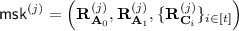• 6. Output and .

On input $\textsf {id}\in \{0,1\}^\ell$, the algorithm does:

• 1. For $\textsf {ID}^{(j)}||\textsf {id}= \textsf {id}[1],...,\textsf {id}[\ell ]$, compute the $\mathbb {Z}_q^{n\times m}$-matrix

  $$\begin{aligned} \mathbf {A}^{(j)}_{C_{\textsf {PRF}}, \textsf {id}}&= \textsf {Eval}(C_{\textsf {PRF}}, \{\mathbf {C}^{(j)}_i\}_{i\in [t]}, \textsf {id}[1]\mathbf {G},...,\textsf {id}[\ell ]\mathbf {G}) \\&= \mathbf {A}^{(j)}\mathbf {R}^{(j)}_{C_{\textsf {PRF}},\textsf {id}} + \textsf {MSB}(\textsf {PRF}(\mathbf {k}^{(j)}, \textsf {id})) \mathbf {G} \\&= \mathbf {A}^{(j)}\mathbf {R}^{(j)}_{C_{\textsf {PRF}},\textsf {id}} + \mu \mathbf {G} \end{aligned}$$

• 2. Set the $\mathbb {Z}_q^{n\times 2m}$-matrix

  $$\begin{aligned} \mathbf {F}_{\textsf {id}, 1-\mu }^{(j)}&= \left[ \mathbf {A}^{(j)} | \mathbf {A}^{(j)}_{1-\mu } - \mathbf {A}^{(j)}_{C_{\textsf {PRF}}, \textsf {id}} \right] \\&= \left[ \mathbf {A}^{(j)} | \mathbf {A} ^{(j)}(\mathbf {R}^{(j)}_{\mathbf {A}_{1-\mu }} - \mathbf {R}^{(j)}_{C_{\textsf {PRF}}, \textsf {id}}) + (1-2\mu )\mathbf {G} ) \right] \\&= \left[ \mathbf {A}^{(j)} | \mathbf {A}^{(j)}\mathbf {R}_{1-\mu }^{(j)} + (1-2\mu )\mathbf {G}\right] \end{aligned}$$

• 3. Run $\textsf {SampleRight}(\mathbf {A}^{(j)}, \mathbf {R}_{1-\mu }^{(j)}, 1-2\mu , \mathbf {G}, s )$ to get a trapdoor $\mathbf {T}^{(j)}_{\textsf {id}}$ for $\mathbf {F}^{(j)}_{\textsf {id}, 1-\mu }$.

• 4. Return $\textsf {sk}_{\textsf {id}}^{(j)} = (1-\mu , \mathbf {T}_{\textsf {id}})$.

The first game Game 0 is the same as the real IND-ID-CPA security game. Game 1 is the same as Game 1 except it runs Sim.Setup and Sim.KeyGen instead of Setup and KeyGen.

Lemma 11

Game 0 and Game 1 are statistically indistinguishable, i.e., there exist a negligible function $\textsf {negl}(\lambda )$ such that $\left| \Pr [S_0] - \Pr [S_1] \right| \le \textsf {negl}(\lambda )$.

Proof

For j-th instance, the differences between Game 0 and Game 1 are:

• 1. In Game 0, $\mathbf {A}^{(j)}$ is generated by TrapGen. By Lemma 5 it has a distribution that is statistically close to uniform distribution on $\mathbb {Z}_q^{n\times m}$. On the other hand, $\mathbf {A}^{(j)}$ is sampled uniformly at random in Game 1.

• 2. By Lemma 2, matrices $\mathbf {A}_0, \mathbf {A}_0, \{\mathbf {C}_i\}_{i\in [t] }$ in Game 1 are statistically close to uniform distribution on $\mathbb {Z}_q^{n\times m}$. In Game 0 those matrices are sampled uniformly from $\mathbb {Z}_q^{n\times m}$.

• 3. In Game 0, the decryption key $\mathbf {T}_{\textsf {id}}^{(j)}$ is sampled by SampleLeft with the trapdoor of $\mathbf {A}^{(j)}$. In Game 1, $\mathbf {T}_{\textsf {id}}^{(j)}$ is sampled by SampleRight with the gadget matrix $\mathbf {G}$ and knowledge of the low-norm matrix $\mathbf {R}^{(j)}_{1-\mu }$. By Lemmas 7 and 8, for sufficiently large s (e.g., $s\ge \sqrt{5}s_1(\mathbf {R}^{(j)}_{1-\mu }) \cdot \omega (\sqrt{\log 2m})$), $\mathbf {T}_{\textsf {id}}^{(j)}$ generated in Game 0 and Game 1 are statistically close.

We therefore conclude that Game 0 and Game 1 are statistically close up to some error $\textsf {negl}(\lambda )$.

Game 2 is the same as Game 1 except that the public matrices $\{\mathbf {A}^{(j)}\}_{j\in [N]}$ for N scheme instances are generated as LWE samples. More specifically, one firstly samples $\mathbf {C}\leftarrow \mathbb {Z}_q^{n'\times n}$. For constructing $\mathbf {A}^{(j)}$, it samples $\mathbf {B}^{(j)} \leftarrow \mathbb {Z}_q^{n'\times m}$, and $\mathbf {F}^{(j)}\leftarrow \chi ^{m\times n}$ and sets $\mathbf {A}^{(j)} = {\mathbf {C}} \cdot \mathbf {B}^{(j)} + {\mathbf {F}^{(j)} } \bmod q$. Here $\mathbf {C}$ serves as the secret of LWE instances for all $\mathbf {A}^{(j)}$. It is easy to see that under the LWE assumption, Game 2 and Game 3 are computationally indistinguishable. So we have the following lemma in which the factor n accounts for a n-step hybrid argument for reducing the LWE problem with matrix secret $\mathbf {C}$ to the LWE problem with single vector secret defined in Definition 3³.

Lemma 12

$\left| \Pr [S_2] - \Pr [S_1] \right| \le n\cdot \textsf {Adv}_{\mathcal {A}_1}^{\textsf {LWE}_{n', q, \chi }}(\lambda )$ for some adversary $\mathcal {A}_1$.

Game 3 is the same as Game 2 except that it answers the encryption query in a slightly different way. Concretely, for encryption query $(k, j, \textsf {id}, \textsf {m}_0, \textsf {m}_1)$ where $k\in [Q_{\textsf {enc}}]$, $j\in [N]$, $\textsf {id}\in \mathcal {ID}$ and $\textsf {m}_0, \textsf {m}_1\in \mathcal {M}$, encryption (of message $\textsf {m}_{\textsf {coin}}$) is done by normal encryption algorithm except the ciphertext component $c^{(j)}_{\mu }$ is chosen uniformly at random from $\{0,1\}^\lambda$, where $\mu = \textsf {MSB}(\textsf {PRF}(\mathbf {k}^{(j)}, \textsf {ID}^{(j)}||\textsf {id}))$. We have the following lemma.

Lemma 13

Game 2 and Game 3 are statistically indistinguishable, i.e., there exists a negligible error $\textsf {negl}(\kappa )$ such that $\left| \Pr [S_3] - \Pr [S_2] \right| \le \textsf {negl}(\kappa )$.

Proof

First of all, we have $\mu = \textsf {MSB}( \textsf {PRF}(\mathbf {k}^{(j)}, \textsf {ID}^{(j)}||\textsf {id})) \in \{0,1\}$. By the construction of encryption algorithm, we have

$$\begin{aligned} \mathbf {F}^{(j)}_{\textsf {id}, \mu }&= [\mathbf {A} ^{(j)} | \mathbf {A}^{(j)}_\mu - \mathbf {A}^{(j)}_{C_{\textsf {PRF}}, \textsf {id}} ] \\&= [\mathbf {A}^{(j)} | (\mathbf {A}^{(j)} \mathbf {R}^{(j)}_{\mathbf {A}_\mu } + \mu \mathbf {G}) - ( \mathbf {A}^{(j)}\mathbf {R}^{(j)}_{C_{\textsf {PRF}}, \textsf {id}} + \textsf {MSB}(\textsf {PRF}(\mathbf {k}^{(j)} , \textsf {ID}^{(j)}||\textsf {id}))\mathbf {G} ) ] \\&= [\mathbf {A}^{(j)} | \mathbf {A}^{(j)} (\mathbf {R}^{(j)}_{\mathbf {A}_\mu } - \mathbf {R}^{(j)}_{C_{\textsf {PRF}}, \textsf {id}} ) ] \\&= [\mathbf {A}^{(j)} | \mathbf {A}^{(j)}{\mathbf {R}_\mu }^{(j)} ] \end{aligned}$$

So for the ciphertext components $(\mathbf {c}'^{(j)}_\mu , {\mathbf {c}_\mu } ^{(j)})$, we have

$$\begin{aligned} {\mathbf {c}_{\mu ,k}'^{(j)} }^\top = {\mathbf {x}_{\mu ,k}^{(j)} } ^\top \cdot \mathbf {F}^{(j)}_{\textsf {id}, \mu } + {\mathbf {e}_{\mu ,k}^{(j)} }^\top \quad ; \quad \mathbf {c}_{\mu ,k}^{(j)} = \textsf {m}_{\textsf {coin}} \oplus \textsf {H}(\mathbf {x}_{\mu ,k}^{(j)}) \end{aligned}$$

where $\mathbf {x}_{\mu ,k}^{(j)}$, $e_{\mu ,k}^{(j)}$ are chosen randomly and freshly for each ciphertext query with index k.⁴ Recall $\mathbf {A}^{(j)} = {\mathbf {C}} \cdot \mathbf {B}^{(j)} + {\mathbf {F}^{(j)} }$ where $\mathbf {B}^{(j)}\in \mathbb {Z}_q^{n'\times m}$ is randomly chosen and $m = 2n\log q + \omega (\log q)$. By Lemma 2, $\mathbf {B}^{(j)}\mathbf {R}_\mu ^{(j)}$ is statistically close to uniform (given $\mathbf {F}^{(j)} \mathbf {R}_{\mu }^{(j)}$) by itself, as required by Theorem 1. Since here we consider the left entropy of randomly and independently chosen $\mathbf {x}_{\mu ,k}^{(j)}$, we can still apply Theorem 1 even though $\mathbf {B}^{(j)}\mathbf {R}_\mu ^{(j)}$ is not statistically uniform given $\mathbf {F}_{\textsf {id}',\mu }^{(j)}$ from another encryption query with $\textsf {id}'\ne \textsf {id}$. By Theorem 1 we get

$$\begin{aligned} {H}_\infty \left( {\mathbf {x}_{\mu ,k}}^{(j)} | {\mathbf {c}_{\mu ,k}'^{(j)} } \right)&\ge H_\infty \left( \mathbf {x}_{\mu ,k}^{(j)} \right) - (n' + 2\kappa )\log q \\&\ge n\log (2\gamma ) - (n' + 2\kappa )\log q \\&\ge \lambda + 2\kappa \end{aligned}$$

By Lemma 1, we have

$$\begin{aligned} \varDelta \left( (\textsf {H}, \textsf {H}(\mathbf {x}_{\mu ,k}^{(j)}) ), (\textsf {H}, \rho _k^{(j)}) \right) \le 2^{-\kappa } = \textsf {negl}(\kappa ) \end{aligned}$$

for uniformly random string $\rho _k^{(j)}\leftarrow \{0,1\}^\lambda$. This makes $\mathbf {c}_{\mu ,k}^{(j)}$ uniformly random and independent of $\textsf {m}_{\textsf {coin}}$.

Game 4 is the same as Game 3 except that it uses Sim.Setup to generate the public parameters. In particular, $\mathbf {A}^{(j)}$ is sampled uniform at random. Looking ahead, this step allows us to run Setup (instead of Sim.Setup) in the next game where we are able to have trapdoor for the matrix $\mathbf {A}^{(j)}$. A straightforward reduction gives us the following lemma.

Lemma 14

$\left| \Pr [S_4] - \Pr [S_3] \right| \le n\cdot \textsf {Adv}_{\mathcal {A}_1}^{\textsf {LWE}_{n', q, \chi }}(\kappa )$ for some adversary $\mathcal {A}_1$.

Game 5 is the same as Game 4 except that it runs algorithms Setup and KeyGen instead of the simulation algorithms. Similar to Lemma 11, we have

Lemma 15

Game 4 and Game 5 are statistically indistinguishable, i.e. $\vert \Pr [S_5] - \Pr [S_4] \vert \le \textsf {negl}(\kappa )$ for some negligible function $\textsf {negl}(\kappa )$.

Game 6 is the same as Game 5 except that the simulator samples the bit value $\mu$ uniformly instead of computing it by PRF as in Game 5. The simulator also keeps the record of tuples $(j, \textsf {id}, \mu )$. For a private key generation query or encryption query on instance j and identity $\textsf {id}$ that has been made before, the simulator simply finds the recorded $\mu$ and uses it for further operations. We prove the following lemma.

Lemma 16

$\left| \Pr [S_6] - \Pr [S_5] \right| \le \textsf {Adv}_{\mathcal {A}_2}^{\textsf {PRF}} (\kappa )$ for some adversary $\mathcal {A}_2$ against PRF.

Proof

We build a simulator $\mathcal {A}_2$ who uses a PRF challenger to simulate Game 5 or Game 6. $\mathcal {A}_2$ flips a fair coin $\textsf {coin}\in \{0,1\}$ and follows $\textsf {Para}(1^\kappa )$ to generate all the parameters of $\textsf {pub}$ except the almost key-homomorphic PRF PRF. Instead, $\mathcal {A}_2$ receives $\textsf {PRF}$ from its challenger.

$\mathcal {A}_2$ chooses N random PRF keys $\{\tilde{\mathbf {k}}^{(j)}\}_{j\in [N]}$. Then it runs Setup to generate except the PRF keys. Notice that has exactly the same distribution as in the real scheme. $\mathcal {A}_2$ answers the following two types of query.

• 1. For a key generation query $(j, \textsf {id})$, $\mathcal {A}_2$ first sends $\textsf {ID}^{(j)}||\textsf {id}$ to its challenger and receives back y. It sets $\mu =\textsf {MSB}\left( y + \textsf {PRF}( \tilde{\mathbf {k}}^{(j)}, \textsf {ID}^{(j)}||\textsf {id}) \right)$ and runs steps 2 to step 5 of KeyGen to generates the private identity key.

• 2. For an encryption query $(k, j, \textsf {id}, \textsf {m}_0, \textsf {m}_1)$, $\mathcal {A}_2$ first sends $\textsf {ID}^{(j)}||\textsf {id}$ to its challenger, receives back y, and sets $\mu = \textsf {MSB}(y + \textsf {PRF}( \tilde{\mathbf {k}}^{(j)}, \textsf {ID}^{(j)}||\textsf {id}))$. It then runs Encrypt to generate ciphertext on message $\textsf {m}_{\textsf {coin}}$ based on the bit value $\mu$, except it samples the component $c_{\mu ,k} ^{(j)}$ randomly.

If $y= \textsf {PRF}(\mathbf {k}^*, \textsf {ID}^{(j)}||\textsf {id})$ for some key $\mathbf {k}^*$, i.e., $\mathcal {A}_2$ interacts with PRF, we have

$$\begin{aligned} \mu&= \textsf {MSB}( y + \textsf {PRF}( \tilde{\mathbf {k}}^{(j)}, \textsf {ID}^{(j)}||\textsf {id}) ) \\&= \textsf {MSB}( \textsf {PRF}(\mathbf {k}^*, \textsf {ID}^{(j)}||\textsf {id}) + \textsf {PRF}( \tilde{\mathbf {k}}^{(j)}, \textsf {ID}^{(j)}||\textsf {id}) ) \\&= \textsf {MSB}(\textsf {PRF}(\mathbf {k}^*\boxplus \tilde{\mathbf {k}}^{(j)}, \textsf {ID}^{(j)}||\textsf {id})) \end{aligned}$$

This shows that $\mathcal {A}_2$ simulates Game 5 with random PRF key $\mathbf {k}^{(j)} = \mathbf {k}^*+ \tilde{\mathbf {k}}^{(j)}$. On the other hand, if $y = F(\textsf {ID}^{(j)}||\textsf {id})$ for some random function $F:\{0,1\}^\ell \rightarrow \{0,1\}^r$, as $F(\cdot )$ is never takes the same input, $\mu$ is uniformly random from the adversary’s view. In this case, $\mathcal {A}_2$ simulates Game 6. Therefore we have $\Pr [S_6] - \Pr [S_5] \le \textsf {Adv}_{\mathcal {A}_2}^{\textsf {PRF}} (\kappa )$.

Let $(\mathbf {c}_{0,k}^{(j)}, {\mathbf {c}'}_{0,k}^{(j)} , \mathbf {c}_{1,k}^{(j)}, {\mathbf {c}'}_{1,k}^{(j)})$ be the challenge ciphertext generated for answering the k-th encryption query $(k, j, \textsf {id}, \textsf {m}_0, \textsf {m}_1)$. Recall that in Game 6, depending on the bit value $\mu = \textsf {MSB}(\textsf {PRF}( \mathbf {k}^{(j)}, \textsf {id}) )$, ${\mathbf {c}_{\mu }}^{(j)}$ is chosen randomly. Game 7 is the same as Game 6 except that it chooses ${\mathbf {c}_{1-\mu ,k}}^{(j)}$ randomly and computes other components honestly. Since $\mu$ is random, we have the following lemma.

Lemma 17

Game 6 and Game 7 are identical, i.e., $\Pr [S_6] = \Pr [S_7]$.

Game 8 is the same as Game 7 except that for encryption and key generation queries on j-th instance and identity id, the bit value $\mu$ is computed as $\mu = \textsf {MSB}( \textsf {PRF}( \mathbf {k}^{(j)}, \textsf {ID}^{(j)}||\textsf {id}) )$. Similar to Lemma 16, we have the following lemma for which we omit the proof as it is identical to the proof of Lemma 16.

Lemma 18

$\left| \Pr [S_7] - \Pr [S_8] \right| \le \textsf {Adv}_{\mathcal {A}_2}^{\textsf {PRF}} (\kappa )$ for some adversary $\mathcal {A}_2$ against PRF.

Game 9 is the same as Game 8 except that the simulation algorithms Sim,Setup and Sim.KeyGen are invoked instead of Setup and KeyGen. Notice that this difference is exactly the difference between Game 0 and Game 1. So we have the following lemma which can be proved using the proof of Lemma 11.

Lemma 19

Game 8 and Game 9 are statistically indistinguishable, i.e., there exist a negligible function $\textsf {negl}(\kappa )$ such that $\left| \Pr [S_9] - \Pr [S_8] \right| \le \textsf {negl}(\kappa )$.

In the next game Game 10, instead of sampling the public matrices $\{\mathbf {A}^{(j)}\}_{j\in [N]}$ for N instances randomly, we again generate them by LWE samples as in Game 2, i.e., $\mathbf {A}^{(j)} = \mathbf {C}\cdot \mathbf {B}^{(j)} + {\mathbf {F}^{(j)}} \bmod q$. This change is not noticeable for efficient adversary under LWE assumption which can be stated by the lemma below.

Lemma 20

$\left| \Pr [S_{10}] - \Pr [S_9] \right| \le n\cdot \textsf {Adv}_{\mathcal {A}_1}^{\textsf {LWE}_{n', q, \chi }}(\kappa )$ for some adversary $\mathcal {A}_1$.

Game 11 is the same as Game 10 except that for any encryption query $(k,j, \textsf {id}, \textsf {m}_0, \textsf {m}_1)$, the ciphertext component ${\mathbf {c}_{\mu ,k}^{(j)}}$ are chosen randomly, where $\mu = \textsf {PRF}(\mathbf {k}^{(j)}, \textsf {ID}^{(j)}||\textsf {id})$. Notice that we have already switched the ciphertext component ${\mathbf {c}_{1-\mu ,k}^{(j)}}$ to random since Game 7. So in Game 11, both ${\mathbf {c}_{0,k}}^{(j)}$ and ${\mathbf {c}_{1,k}}^{(j)}$ (which were used to mask the message $\textsf {m}_{\textsf {coin}}$) are random, meaning that the challenge ciphertexts replied to encryption queries are random and independent of the messages chosen by the adversary. So the adversary has no advantage in wining Game 11. The proof of the following lemma is omitted as it is the same as the proof of Lemma 13.

Lemma 21

Game 10 is statistically close to Game 11, and in Game 11, no adversary has any advantage in guessing the bit $\textsf {coin}$, i.e., $\left| \Pr [S_{11}] - \Pr [S_{10}]\right| \le \textsf {negl}(\kappa )$ for some statistically error $negl(\kappa )$ and $\Pr [S_{11}] = 1/2$.

To sum up, we have:

$$\begin{aligned} \textsf {Adv}^{\textsf {IND-ID-CPA}}_{\varPi , \mathcal {A}, (N, Q_{\textsf {key}}, Q_{\textsf {enc}})} (\kappa )&= \left| \Pr [S_1] - 1/2 \right| \\&= \vert \Pr [S_1] - \Pr [S_{11}] \vert \\&\le \sum \nolimits _{i=0}^{10}\vert \Pr [S_{i}] - \Pr [S_{i+1}] \vert \\&= 3n \cdot \textsf {Adv}_{\mathcal {A}_1}^{\textsf {LWE}_{n', q, \chi }} + 2\cdot \textsf {Adv}_{\mathcal {A}_2}^{\textsf {PRF}}(\kappa ) + \textsf {negl}(\kappa ) \end{aligned}$$

for some function $\textsf {negl}(\kappa )$ which stands for the negligible statistical error in the reduction. The security loss is independent of the number of instances N, the number of encryption queries $Q_{\textsf {enc}}$ and the number of key generation queries $Q_{\textsf {key}}$.

5 Discussion and Conclusion

For generality, we reduce the security of the IBE scheme to the LWE problem $\textsf {LWE}_{n',q,\chi }$ and the security of the PRF as shown by Theorem 2. To make the whole IBE scheme (almost) tightly secure, we need (almost) tightly secure PRFs. The instantiation of PRF also affects the LWE problem $\textsf {LWE}_{n',q,\chi }$ quantitatively by the depth d of the circuit $C_{\textsf {PRF}}$. For example, employing an almost tightly secure (based on the LWE problem) BLMR-PRF [10] allows us to use a polynomial modulo q. Meanwhile, the computational assumption we make for the PRF affects the final assumption that we need to make for the IBE scheme. The (almost) tight security proof of the BLMR-PRF requires an LWE assumption with modulus-to-noise ratio $n^{\Omega (\ell )}$ ($\ell$ is the PRF input length) which is quantitatively stronger than the LWE problem $\textsf {LWE}_{n',q,\chi }$ we use for the LWE lossy mode. This means the IBE scheme needs a strong LWE assumption on which the BLMR-PRF is based. However any future improvement in (lattice-based) key-homomorphic PRFs will directly improve the efficiency and security of our scheme without weakening the underlying assumption.

Under a suitable BLMR-PRF instantiation, our IBE scheme, based on a strong LWE assumption (sub-exponential modulus-to-noise ratio), achieves almost tight security in the strong MIMC setting. Under the same assumption, the Boyen-Li IBE scheme from [11] (using almost tightly secure PRFs from [5, 10]) only had an almost tight security reduction in the SISC setting. The (strong) LWE assumption that we use is believed to be hard and has been widely used in other contexts, including fully-homomorphic encryption [14], attribute-based/predicate encryption [9, 21, 22] and lattice-based constrained PRFs [13, 15]. How to obtain an (almost) tightly secure IBE scheme in the MIMC setting was not known before, even with such a strong LWE assumption. By applying the standard BCHK transformation [8] with tightly secure one-time signature schemes (e.g., [7]), our IBE scheme leads to the first almost tightly CCA2 secure public-key encryption scheme from lattices in the multi-instance and multi-ciphertext setting [23].

Our work motivates two future directions: to improve efficiency and key sizes; and to design tightly secure key-homomorphic PRFs from weaker assumptions.

References

Agrawal, S., Boneh, D., Boyen, X.: Efficient lattice (H)IBE in the standard model. In: Gilbert, H. (ed.) EUROCRYPT 2010. LNCS, vol. 6110, pp. 553–572. Springer, Heidelberg (2010). https://doi.org/10.1007/978-3-642-13190-5_28
Ajtai, M.: Generating hard instances of lattice problems (extended abstract). In: STOC, pp. 99–108 (1996)
Alwen, J., Krenn, S., Pietrzak, K., Wichs, D.: Learning with rounding, revisited. In: Canetti, R., Garay, J.A. (eds.) CRYPTO 2013. LNCS, vol. 8042, pp. 57–74. Springer, Heidelberg (2013). https://doi.org/10.1007/978-3-642-40041-4_4
Attrapadung, N., Hanaoka, G., Yamada, S.: A framework for identity-based encryption with almost tight security. In: Iwata, T., Cheon, J.H. (eds.) ASIACRYPT 2015. LNCS, vol. 9452, pp. 521–549. Springer, Heidelberg (2015). https://doi.org/10.1007/978-3-662-48797-6_22
Banerjee, A., Peikert, C., Rosen, A.: Pseudorandom functions and lattices. In: Pointcheval, D., Johansson, T. (eds.) EUROCRYPT 2012. LNCS, vol. 7237, pp. 719–737. Springer, Heidelberg (2012). https://doi.org/10.1007/978-3-642-29011-4_42
Bellare, M., Kiltz, E., Peikert, C., Waters, B.: Identity-based (lossy) trapdoor functions and applications. In: Pointcheval, D., Johansson, T. (eds.) EUROCRYPT 2012. LNCS, vol. 7237, pp. 228–245. Springer, Heidelberg (2012). https://doi.org/10.1007/978-3-642-29011-4_15
Blazy, O., Kakvi, S.A., Kiltz, E., Pan, J.: Tightly-secure signatures from chameleon hash functions. In: Katz, J. (ed.) PKC 2015. LNCS, vol. 9020, pp. 256–279. Springer, Heidelberg (2015). https://doi.org/10.1007/978-3-662-46447-2_12
Boneh, D., Canetti, R., Halevi, S., Katz, J.: Chosen-ciphertext security from identity-based encryption. SIAM J. Comput. 36(5), 1301–1328 (2006)
Boneh, D., Gentry, C., Gorbunov, S., Halevi, S., Nikolaenko, V., Segev, G., Vaikuntanathan, V., Vinayagamurthy, D.: Fully key-homomorphic encryption, arithmetic circuit ABE and compact garbled circuits. In: Nguyen, P.Q., Oswald, E. (eds.) EUROCRYPT 2014. LNCS, vol. 8441, pp. 533–556. Springer, Heidelberg (2014). https://doi.org/10.1007/978-3-642-55220-5_30
Boneh, D., Lewi, K., Montgomery, H., Raghunathan, A.: Key homomorphic PRFs and their applications. In: Canetti, R., Garay, J.A. (eds.) CRYPTO 2013. LNCS, vol. 8042, pp. 410–428. Springer, Heidelberg (2013). https://doi.org/10.1007/978-3-642-40041-4_23
Boyen, X., Li, Q.: Towards tightly secure lattice short signature and id-based encryption. In: Cheon, J.H., Takagi, T. (eds.) ASIACRYPT 2016. LNCS, vol. 10032, pp. 404–434. Springer, Heidelberg (2016). https://doi.org/10.1007/978-3-662-53890-6_14
Boyen, X., Li, Q.: All-but-many lossy trapdoor functions from lattices and applications. In: Katz, J., Shacham, H. (eds.) CRYPTO 2017. LNCS, vol. 10403, pp. 298–331. Springer, Cham (2017). https://doi.org/10.1007/978-3-319-63697-9_11
Brakerski, Z., Tsabary, R., Vaikuntanathan, V., Wee, H.: Private constrained PRFs (and more) from LWE. In: Kalai, Y., Reyzin, L. (eds.) TCC 2017. LNCS, vol. 10677, pp. 264–302. Springer, Cham (2017). https://doi.org/10.1007/978-3-319-70500-2_10
Brakerski, Z., Vaikuntanathan, V.: Efficient fully homomorphic encryption from (standard) LWE. In: FOCS, pp. 97–106 (2011)
Brakerski, Z., Vaikuntanathan, V.: Constrained key-homomorphic PRFs from standard lattice assumptions. In: Dodis, Y., Nielsen, J.B. (eds.) TCC 2015. LNCS, vol. 9015, pp. 1–30. Springer, Heidelberg (2015). https://doi.org/10.1007/978-3-662-46497-7_1
Cash, D., Hofheinz, D., Kiltz, E., Peikert, C.: Bonsai trees, or how to delegate a lattice basis. J. Cryptol. 25(4), 601–639 (2012)
Chen, J., Gong, J., Weng, J.: Tightly secure IBE under constant-size master public key. In: Fehr, S. (ed.) PKC 2017. LNCS, vol. 10174, pp. 207–231. Springer, Heidelberg (2017). https://doi.org/10.1007/978-3-662-54365-8_9
Gentry, C., Peikert, C., Vaikuntanathan, V.: Trapdoors for hard lattices and new cryptographic constructions. In: STOC, pp. 197–206 (2008)
Gong, J., Chen, J., Dong, X., Cao, Z., Tang, S.: Extended nested dual system groups, revisited. In: Cheng, C.-M., Chung, K.-M., Persiano, G., Yang, B.-Y. (eds.) PKC 2016. LNCS, vol. 9614, pp. 133–163. Springer, Heidelberg (2016). https://doi.org/10.1007/978-3-662-49384-7_6
Gong, J., Dong, X., Chen, J., Cao, Z.: Efficient IBE with tight reduction to standard assumption in the multi-challenge setting. In: Cheon, J.H., Takagi, T. (eds.) ASIACRYPT 2016. LNCS, vol. 10032, pp. 624–654. Springer, Heidelberg (2016). https://doi.org/10.1007/978-3-662-53890-6_21
Gorbunov, S., Vaikuntanathan, V., Wee, H.: Attribute-based encryption for circuits. In: STOC, pp. 545–554 (2013)
Gorbunov, S., Vaikuntanathan, V., Wee, H.: Predicate encryption for circuits from LWE. In: Gennaro, R., Robshaw, M. (eds.) CRYPTO 2015. LNCS, vol. 9216, pp. 503–523. Springer, Heidelberg (2015). https://doi.org/10.1007/978-3-662-48000-7_25
Hofheinz, D., Jager, T.: Tightly secure signatures and public-key encryption. In: Safavi-Naini, R., Canetti, R. (eds.) CRYPTO 2012. LNCS, vol. 7417, pp. 590–607. Springer, Heidelberg (2012). https://doi.org/10.1007/978-3-642-32009-5_35
Hofheinz, D., Koch, J., Striecks, C.: Identity-based encryption with (almost) tight security in the multi-instance, multi-ciphertext setting. In: Katz, J. (ed.) PKC 2015. LNCS, vol. 9020, pp. 799–822. Springer, Heidelberg (2015). https://doi.org/10.1007/978-3-662-46447-2_36
Libert, B., Sakzad, A., Stehlé, D., Steinfeld, R.: All-but-many lossy trapdoor functions and selective opening chosen-ciphertext security from LWE. In: Katz, J., Shacham, H. (eds.) CRYPTO 2017. LNCS, vol. 10403, pp. 332–364. Springer, Cham (2017). https://doi.org/10.1007/978-3-319-63697-9_12
Micciancio, D., Peikert, C.: Trapdoors for lattices: simpler, tighter, faster, smaller. In: Pointcheval, D., Johansson, T. (eds.) EUROCRYPT 2012. LNCS, vol. 7237, pp. 700–718. Springer, Heidelberg (2012). https://doi.org/10.1007/978-3-642-29011-4_41
Peikert, C., Waters, B.: Lossy trapdoor functions and their applications. SIAM J. Comput. 40(6), 1803–1844 (2011)
Regev, O.: On lattices, learning with errors, random linear codes, and cryptography. In: STOC, pp. 84–93 (2005)
Author information
Authors and Affiliations
Corresponding author
Editor information
Editors and Affiliations
Rights and permissions
Copyright information
© 2018 Springer International Publishing AG, part of Springer Nature
About this paper
Cite this paper
Boyen, X., Li, Q. (2018). Almost Tight Multi-Instance Multi-Ciphertext Identity-Based Encryption on Lattices. In: Preneel, B., Vercauteren, F. (eds) Applied Cryptography and Network Security. ACNS 2018. Lecture Notes in Computer Science(), vol 10892. Springer, Cham. https://doi.org/10.1007/978-3-319-93387-0_28
Download citation
DOI: https://doi.org/10.1007/978-3-319-93387-0_28
Published:
Publisher Name: Springer, Cham
Print ISBN: 978-3-319-93386-3
Online ISBN: 978-3-319-93387-0
eBook Packages: Computer ScienceComputer Science (R0)