Explicit Effect Subtyping

Abstract

As popularity of algebraic effects and handlers increases, so does a demand for their efficient execution. Eff, an ML-like language with native support for handlers, has a subtyping-based effect system on which an effect-aware optimizing compiler could be built. Unfortunately, in our experience, implementing optimizations for Eff is overly error-prone because its core language is implicitly-typed, making code transformations very fragile.

To remedy this, we present an explicitly-typed polymorphic core calculus for algebraic effect handlers with a subtyping-based type-and-effect system. It reifies appeals to subtyping in explicit casts with coercions that witness the subtyping proof, quickly exposing typing bugs in program transformations.

Our typing-directed elaboration comes with a constraint-based inference algorithm that turns an implicitly-typed Eff-like language into our calculus. Moreover, all coercions and effect information can be erased in a straightforward way, demonstrating that coercions have no computational content.

1 Introduction

Algebraic effect handlers [17, 18] are quickly maturing from a theoretical model to a practical language feature for user-defined computational effects. Yet, in practice they still incur a significant performance overhead compared to native effects.

Our earlier efforts [22] to narrow this gap with an optimising compiler from Eff [2] to OCaml showed promising results, in some cases reaching even the performance of hand-tuned code, but were very fragile and have been postponed until a more robust solution is found. We believe the main reason behind this fragility is the complexity of subtyping in combination with the implicit typing of Eff’s core language, further aggravated by the “garbage collection” of subtyping constraints (see Sect. 7).¹

For efficient compilation, one must avoid the poisoning problem [26], where unification forces a pure computation to take the less precise impure type of the context (e.g. a pure and an impure branch of a conditional both receive the same impure type). Since this rules out existing (and likely simpler) effect systems for handlers based on row-polymorphism [8, 12, 14], we propose a polymorphic explicitly-typed calculus based on subtyping. More specifically, our contributions are as follows:

• First, in Sect. 3 we present ImpEff, a polymorphic implicitly-typed calculus for algebraic effects and handlers with a subtyping-based type-and-effect system. ImpEff is essentially a (desugared) source language as it appears in the compiler frontend of a language like Eff.

• Next, Sect. 4 presents ExEff, the core calculus, which combines explicit System F-style polymorphism with explicit coercions for subtyping in the style of Breazu-Tannen et al. [3]. This calculus comes with a type-and-effect system, a small-step operational semantics and a proof of type-safety.

• Section 5 specifies the typing-directed elaboration of ImpEff into ExEff and presents a type inference algorithm for ImpEff that produces the elaborated ExEff term as a by-product. It also establishes that the elaboration preserves typing, and that the algorithm is sound with respect to the specification and yields principal types.

• Finally, Sect. 6 defines SkelEff, which is a variant of ExEff without effect information or coercions. SkelEff is also representative of Multicore Ocaml’s support for algebraic effects and handlers [6], which is a possible compilation target of Eff. By showing that the erasure from ExEff to SkelEff preserves semantics, we establish that ExEff’s coercions are computationally irrelevant and that, despite the existence of multiple proofs for the same subtyping, there is no coherence problem. To enable erasure, ExEff annotates its types with (type) skeletons, which capture the erased counterpart and are, to our knowledge, a novel contribution.

• Our paper comes with two software artefacts: an ongoing implementation² of a compiler from Eff to OCaml with ExEff at its core, and an Abella mechanisation³ of Theorems 1, 2, 6, and 7. Remaining theorems all concern the inference algorithm, and their proofs closely follow [20].

The full version of this paper includes an appendix with omitted figures and can be found at http://www.cs.kuleuven.be/publicaties/rapporten/cw/CW711.abs.html.

2 Overview

This section presents an informal overview of the ExEff calculus, and the main issues with elaborating to and erasing from it.

2.1 Algebraic Effect Handlers

The main premise of algebraic effects is that impure behaviour arises from a set of operations such as $\mathtt {Get}$ and $\mathtt {Set}$ for mutable store, $\mathtt {Read}$ and $\mathtt {Print}$ for interactive input and output, or $\mathtt {Raise}$ for exceptions [17]. This allows generalizing exception handlers to other effects, to express backtracking, co-operative multithreading and other examples in a natural way [2, 18].

Assume operations $\mathtt {Tick} : \mathtt {Unit}\rightarrow \mathtt {Unit}$ and $\mathtt {Tock} : \mathtt {Unit}\rightarrow \mathtt {Unit}$ that take a unit value as a parameter and yield a unit value as a result. Unlike special built-in operations, these operations have no intrinsic effectful behaviour, though we can give one through handlers. For example, the handler replaces all calls of $\mathtt {Tick}$ by printing out “tick” and similarly for $\mathtt {Tock}$. But there is one significant difference between the two cases. Unlike exceptions, which always abort the evaluation, operations have a continuation waiting for their result. It is this continuation that the handler captures in the variable k and potentially uses in the handling clause. In the clause for $\mathtt {Tick}$, the continuation is resumed by passing it the expected unit value, whereas in the clause for $\mathtt {Tock}$, the operation is discarded. Thus, if we handle a computation emitting the two operations, it will print out “tick” until a first “tock” is printed, after which the evaluation stops.

2.2 Elaborating Subtyping

Consider the computation $\mathtt {do}~{x} \leftarrow {\mathtt {Tick}~{\mathtt {unit}}} ;{f~x}$ and assume that f has the function type $\mathtt {Unit}\rightarrow \mathtt {Unit}~!~\{\mathtt {Tock}\}$, taking unit values to unit values and perhaps calling $\mathtt {Tock}$ operations in the process. The whole computation then has the type $\mathtt {Unit}~!~\{\mathtt {Tick},\mathtt {Tock}\}$ as it returns the unit value and may call $\mathtt {Tick}$ and $\mathtt {Tock}$.

The above typing implicitly appeals to subtyping in several places. For instance, $\mathtt {Tick}~{\mathtt {unit}}$ has type $\mathtt {Unit}~!~\{\mathtt {Tick}\}$ and f x type $\mathtt {Unit}~!~\{\mathtt {Tock}\}$. Yet, because they are sequenced with $\mathtt {do}$, the type system expects they have the same set of effects. The discrepancies are implicitly reconciled by the subtyping which admits both $\{\mathtt {Tick}\} \leqslant \{\mathtt {Tick},\mathtt {Tock}\}$ and $\{\mathtt {Tock}\} \leqslant \{\mathtt {Tick},\mathtt {Tock}\}$.

We elaborate the ImpEff term into the explicitly-typed core language ExEff to make those appeals to subtyping explicit by means of casts with coercions:

$$ \mathtt {do}~{x} \leftarrow {({(\mathtt {Tick}~{\mathtt {unit}})} \vartriangleright {\gamma _1})} ;{{(f~x)} \vartriangleright {\gamma _2}} $$

A coercion $\gamma$ is a witness for a subtyping $A~!~\varDelta \leqslant A'~!~\varDelta '$ and can be used to cast a term c of type $A~!~\varDelta$ to a term ${c} \vartriangleright {\gamma }$ of type $A'~!~\varDelta '$. In the above term, $\gamma _1$ and $\gamma _2$ respectively witness $\mathtt {Unit}~!~\{\mathtt {Tick}\} \leqslant \mathtt {Unit}~!~\{\mathtt {Tick},\mathtt {Tock}\}$ and $\mathtt {Unit}~!~\{\mathtt {Tock}\} \leqslant \mathtt {Unit}~!~\{\mathtt {Tick},\mathtt {Tock}\}$.

2.3 Polymorphic Subtyping for Types and Effects

The above basic example only features monomorphic types and effects. Yet, our calculus also supports polymorphism, which makes it considerably more expressive. For instance the type of $f$ in $\mathtt {let}~{ f } = {(\mathtt {fun}~{g} \mapsto {g~\mathtt {unit}})}~\mathtt {in}~{\ldots }$ is generalised to:

$$ \forall \alpha , \alpha '.\forall \delta ,\delta '.\alpha \leqslant \alpha '\Rightarrow \delta \leqslant \delta ' \Rightarrow (\mathtt {Unit}\rightarrow \alpha ~!~\delta ) \rightarrow \alpha ' ~!~ \delta ' $$

This polymorphic type scheme follows the qualified types convention [9] where the type $(\mathtt {Unit}\rightarrow \alpha ~!~\delta ) \rightarrow \alpha ' ~!~ \delta '$ is subjected to several qualifiers, in this case $\alpha \leqslant \alpha '$ and $\delta \leqslant \delta '$. The universal quantifiers on the outside bind the type variables $\alpha$ and $\alpha '$, and the effect set variables $\delta$ and $\delta '$.

The elaboration of f into ExEff introduces explicit binders for both the quantifiers and the qualifiers, as well as the explicit casts where subtyping is used.

$$\begin{aligned} \varLambda \alpha .\varLambda \alpha '\!\!.\varLambda \delta .\varLambda \delta '\!\!.\varLambda (\omega \!:\!\alpha \leqslant \alpha '). \varLambda (\omega '\!:\!\delta \leqslant \delta '). \mathtt {fun}~{(g\!:\!\mathtt {Unit}\rightarrow \alpha \,!\, \delta )\!} \mapsto {\!{(g\,\mathtt {unit})\!} \vartriangleright {\!(\omega \,!\,\omega ')}} \end{aligned}$$

Here the binders for qualifiers introduce coercion variables $\omega$ between pure types and $\omega '$ between operation sets, which are then combined into a computation coercion $\omega ~!~\omega '$ and used for casting the function application $g\,\mathtt {unit}$ to the expected type.

Suppose that h has type $\mathtt {Unit}\rightarrow \mathtt {Unit}\,!\,\{\mathtt {Tick}\}$ and $f\,h$ type $\mathtt {Unit}\,!\,\{\mathtt {Tick},\mathtt {Tock}\}$. In the ExEff calculus the corresponding instantiation of f is made explicit through type and coercion applications

$$ f\,\mathtt {Unit}\,\mathtt {Unit}\,\{\mathtt {Tick}\}\,\{\mathtt {Tick},\mathtt {Tock}\}\,\gamma _1\,\gamma _2\,h $$

where $\gamma _1$ needs to be a witness for $\mathtt {Unit}\leqslant \mathtt {Unit}$ and $\gamma _2$ for $\{\mathtt {Tick}\} \leqslant \{\mathtt {Tick},\mathtt {Tock}\}$.

2.4 Guaranteed Erasure with Skeletons

One of our main requirements for ExEff is that its effect information and subtyping can be easily erased. The reason is twofold. Firstly, we want to show that neither plays a role in the runtime behaviour of ExEff programs. Secondly and more importantly, we want to use a conventionally typed (System F-like) functional language as a backend for the Eff compiler.

At first, erasure of both effect information and subtyping seems easy: simply drop that information from types and terms. But by dropping the effect variables and subtyping constraints from the type of $f$, we get $\forall \alpha , \alpha '. (\mathtt {Unit}\rightarrow \alpha ) \rightarrow \alpha '$ instead of the expected type $\forall \alpha . (\mathtt {Unit}\rightarrow \alpha ) \rightarrow \alpha$. In our naive erasure attempt we have carelessly discarded the connection between $\alpha$ and $\alpha '$. A more appropriate approach to erasure would be to unify the types in dropped subtyping constraints. However, unifying types may reduce the number of type variables when they become instantiated, so corresponding binders need to be dropped, greatly complicating the erasure procedure and its meta-theory.

Fortunately, there is an easier way by tagging all bound type variables with skeletons, which are barebone types without effect information. For example, the skeleton of a function type $A \rightarrow B~!~\varDelta$ is $\tau _1 \rightarrow \tau _2$, where $\tau _1$ is the skeleton of A and $\tau _2$ the skeleton of B. In ExEff every well-formed type has an associated skeleton, and any two types $A_1 \leqslant A_2$ share the same skeleton. In particular, binders for type variables are explicitly annotated with skeleton variables $\varsigma$. For instance, the actual type of $f$ is:

$$ \forall \varsigma .\forall (\alpha :\varsigma ), (\alpha ':\varsigma ).\forall \delta ,\delta '.\alpha \leqslant \alpha '\Rightarrow \delta \leqslant \delta ' \Rightarrow (\mathtt {Unit}\rightarrow \alpha ~!~\delta ) \rightarrow \alpha ' ~!~ \delta ' $$

The skeleton quantifications and annotations also appear at the term-level:

$$\begin{aligned} \varLambda \varsigma . \varLambda (\alpha :\varsigma ).\varLambda (\alpha ':\varsigma ).\varLambda \delta .\varLambda \delta '. \varLambda (\omega : \alpha \leqslant \alpha '). \varLambda (\omega ': \delta \leqslant \delta '). \ldots \end{aligned}$$

Now erasure is really easy: we drop not only effect and subtyping-related term formers, but also type binders and application. We do retain skeleton binders and applications, which take over the role of (plain) types in the backend language. In terms, we replace types by their skeletons. For instance, for $f$ we get:

$$\begin{aligned} \varLambda \varsigma . \mathtt {fun}~{(g : \mathtt {Unit}\rightarrow \varsigma )} \mapsto {g\,\mathtt {unit}} ~~:~~ \forall \varsigma . (\mathtt {Unit}\rightarrow \varsigma ) \rightarrow \varsigma \end{aligned}$$

Fig. 1.

ImpEff Syntax

3 The ImpEff Language

This section presents ImpEff, a basic functional calculus with support for algebraic effect handlers, which forms the core language of our optimising compiler. We describe the relevant concepts, but refer the reader to Pretnar’s tutorial [21], which explains essentially the same calculus in more detail.

3.1 Syntax

Figure 1 presents the syntax of the source language. There are two main kinds of terms: (pure) values v and (dirty) computations c, which may call effectful operations. Handlers h are a subsidiary sort of values. We assume a given set of operations $\mathtt {Op}$, such as $\mathtt {Get}$ and $\mathtt {Put}$. We abbreviate ${{\mathtt {Op}_1}\,{x}\,{k}} \mapsto c_{\mathtt {Op}_1}, \ldots , {{\mathtt {Op}_n}\,{x}\,{k}} \mapsto c_{\mathtt {Op}_n}$ as $[{{\mathtt {Op}}\,{x}\,{k}} \mapsto c_\mathtt {Op}]_{\mathtt {Op}\in \mathcal {O}}$, and write $\mathcal {O}$ to denote the set $\{ \mathtt {Op}_1, \dots , \mathtt {Op}_n \}$.

Similarly, we distinguish between two basic sorts of types: the value types A, B and the computation types $\underline{C}, \underline{D}$. There are four forms of value types: type variables $\alpha$, function types $A \rightarrow \underline{C}$, handler types $\underline{C}\Rrightarrow \underline{D}$ and the $\mathtt {Unit}$ type. Skeletons $\tau$ capture the shape of types, so, by design, their forms are identical. The computation type $A \mathrel {!}\varDelta$ is assigned to a computation returning values of type A and potentially calling operations from the dirt set $\varDelta$. A dirt set contains zero or more operations $\mathtt {Op}$ and is terminated either by an empty set or a dirt variable $\delta$. Though we use cons-list syntax, the intended semantics of dirt sets $\varDelta$ is that the order of operations $\mathtt {Op}$ is irrelevant. Similarly to all HM-based systems, we discriminate between value types (or monotypes) A, qualified types $K$ and polytypes (or type schemes) $S$. (Simple) subtyping constraints $\pi$ denote inequalities between either value types or dirts. We also present the more general form of constraints $\rho$ that includes inequalities between computation types (as we illustrate in Sect. 3.2 below, this allows for a single, uniform constraint entailment relation). Finally, polytypes consist of zero or more skeleton, type or dirt abstractions followed by a qualified type.

Fig. 2.

ImpEff Typing & Elaboration

3.2 Typing

Figure 2 presents the typing rules for values and computations, along with a typing-directed elaboration into our target language ExEff. In order to simplify the presentation, in this section we focus exclusively on typing. The parts of the rules that concern elaboration are highlighted in gray and are discussed in Sect. 5.

Values. Typing for values takes the form , and, given a typing environment $\varGamma$, checks a value v against a value type A.

Rule TmVar handles term variables. Given that x has type $(\forall \overline{\varsigma }. \overline{\alpha :\tau }. \forall \overline{\delta }. \overline{\pi } \Rightarrow A )$, we appropriately instantiate the skeleton ($\overline{\varsigma }$), type ($\overline{\alpha }$), and dirt ($\overline{\delta }$) variables, and ensure that the instantiated wanted constraints $\overline{\sigma (\pi )}$ are satisfied, via side condition . Rule TmCastV allows casting the type of a value v from $A$ to $B$, if $A$ is a subtype of $B$ (upcasting). As illustrated by Rule TmTmAbs, we omit freshness conditions by adopting the Barendregt convention [1]. Finally, Rule TmHand gives typing for handlers. It requires that the right-hand sides of the return clause and all operation clauses have the same computation type ($B \,!\,\varDelta$), and that all operations mentioned are part of the top-level signature $\varSigma$.⁴ The result type takes the form $A ~!~\varDelta \,\cup \,\mathcal {O}\Rrightarrow B ~!~\varDelta$, capturing the intended handler semantics: given a computation of type $A ~!~\varDelta \cup \mathcal {O}$, the handler (a) produces a result of type $B$, (b) handles operations $\mathcal {O}$, and (c) propagates unhandled operations $\varDelta$ to the output.

Computations. Typing for computations takes the form , and, given a typing environment $\varGamma$, checks a computation c against a type $\underline{C}$.

Rule TmCastC behaves like Rule TmCastV, but for computation types. Rule TmLet handles polymorphic, non-recursive let-bindings. Rule TmReturn handles $\mathtt {return}~{v}$ computations. Keyword $\mathtt {return}\;$ effectively lifts a value v of type $A$ into a computation of type $A ~!~\emptyset$. Rule TmOp checks operation calls. First, we ensure that v has the appropriate type, as specified by the signature of $\mathtt {Op}$. Then, the continuation (y.c) is checked. The side condition $\mathtt {Op}\in \varDelta$ ensures that the called operation $\mathtt {Op}$ is captured in the result type. Rule TmDo handles sequencing. Given that $c_1$ has type $A \,!\,\varDelta$, the pure part of the result of type $A$ is bound to term variable x, which is brought in scope for checking $c_2$. As we mentioned in Sect. 2, all computations in a $\texttt {do}$-construct should have the same effect set, $\varDelta$. Rule TmHandle eliminates handler types, just as Rule TmTmApp eliminates arrow types.

Fig. 3.

ImpEff Constraint Entailment

Fig. 4.

ExEff Syntax

Constraint Entailment. The specification of constraint entailment takes the form and is presented in Fig. 3. Notice that we use $\rho$ instead of $\pi$, which allows us to capture subtyping between two value types, computation types or dirts, within the same relation. Subtyping can be established in several ways:

Rule CoVar handles given assumptions. Rules VCoRefl and DCoRefl express that subtyping is reflexive, for both value types and dirts. Notice that we do not have a rule for the reflexivity of computation types since, as we illustrate below, it can be established using the reflexivity of their subparts. Rules VCoTrans, CCoTrans and DCoTrans express the transitivity of subtyping for value types, computation types and dirts, respectively. Rule VCoArr establishes inequality of arrow types. As usual, the arrow type constructor is contravariant in the argument type. Rules VCoArrL and CCoArrR are the inversions of Rule VCoArr, allowing us to establish the relation between the subparts of the arrow types. Rules VCoHand, CCoHL, and CCoHR work similarly, for handler types. Rule CCoComp captures the covariance of type constructor (!), establishing subtyping between two computation types if subtyping is established for their respective subparts. Rules VCoPure and DCoImpure are its inversions. Finally, Rules DCoNil and DCoOp establish subtyping between dirts. Rule DCoNil captures that the empty dirty set $\emptyset$ is a subdirt of any dirt $\varDelta$ and Rule DCoOp expresses that dirt subtyping preserved under extension with the same operation $\mathtt {Op}$.

Well-Formedness of Types, Constraints, Dirts, and Skeletons. The relations and check the well-formedness of value and computation types respectively. Similarly, relations and check the well-formedness of constraints and dirts, respectively.

4 The ExEff Language

4.1 Syntax

Figure 4 presents ExEff’s syntax. ExEff is an intensional type theory akin to System F  [7], where every term encodes its own typing derivation. In essence, all abstractions and applications that are implicit in ImpEff, are made explicit in ExEff via new syntactic forms. Additionally, ExEff is impredicative, which is reflected in the lack of discrimination between value types, qualified types and type schemes; all non-computation types are denoted by $T$. While the impredicativity is not strictly required for the purpose at hand, it makes for a cleaner system.

Coercions. Of particular interest is the use of explicit subtyping coercions, denoted by $\gamma$. ExEff uses these to replace the implicit casts of ImpEff (Rules TmCastV and TmCastC in Fig. 2) with explicit casts $({v} \vartriangleright {\gamma })$ and $({c} \vartriangleright {\gamma })$.

Essentially, coercions $\gamma$ are explicit witnesses of subtyping derivations: each coercion form corresponds to a subtyping rule. Subtyping forms a partial order, which is reflected in coercion forms ${\gamma _1} \gg {\gamma _2}$, $\langle { T } \rangle$, and $\langle {\varDelta } \rangle$. Coercion form ${\gamma _1} \gg {\gamma _2}$ captures transitivity, while forms $\langle { T } \rangle$ and $\langle {\varDelta } \rangle$ capture reflexivity for value types and dirts (reflexivity for computation types can be derived from these).

Subtyping for skeleton abstraction, type abstraction, dirt abstraction, and qualification is witnessed by forms $\forall \varsigma . \gamma$, $\forall \alpha . \gamma$, $\forall \delta . \gamma$, and $\pi \Rightarrow \gamma$, respectively. Similarly, forms ${\gamma }[{\tau }]$, ${\gamma }[{ T }]$, ${\gamma }[{\varDelta }]$, and ${\gamma _1}@{\gamma _2}$ witness subtyping of skeleton instantiation, type instantiation, dirt instantiation, and coercion application, respectively.

Syntactic forms $\gamma _1 \rightarrow \gamma _2$ and $\gamma _1 \Rrightarrow \gamma _2$ capture injection for the arrow and the handler type constructor, respectively. Similarly, inversion forms $\textit{left}({\gamma })$ and $\textit{right}({\gamma })$ capture projection, following from the injectivity of both type constructors.

Coercion form $\gamma _1~!~\gamma _2$ witnesses subtyping for computation types, using proofs for their components. Inversely, syntactic forms $\textit{pure}({\gamma })$ and $\textit{impure}({\gamma })$ witness subtyping between the value- and dirt-components of a computation coercion.

Finally, coercion forms $\emptyset _\varDelta$ and $\{\mathtt {Op}\}\,\cup \,\gamma$ are concerned with dirt subtyping. Form $\emptyset _\varDelta$ witnesses that the empty dirt $\emptyset$ is a subdirt of any dirt $\varDelta$. Lastly, coercion form $\{\mathtt {Op}\}\,\cup \,\gamma$ witnesses that subtyping between dirts is preserved under extension with a new operation. Note that we do not have an inversion form to extract a witness for $\varDelta _1 \leqslant \varDelta _2$ from a coercion for $\{\mathtt {Op}\}\,\cup \,\varDelta _1 \leqslant \{\mathtt {Op}\}\,\cup \,\varDelta _2$. The reason is that dirt sets are sets and not inductive structures. For instance, for $\varDelta _1 = \{ \mathtt {Op}\}$ and $\varDelta _2 = \emptyset$ the latter subtyping holds, but the former does not.

Fig. 5.

ExEff Value Typing

4.2 Typing

Value and Computation Typing. Typing for ExEff values and computations is presented in Figs. 5 and 6 and is given by two mutually recursive relations of the form ${\varGamma } \vdash _{{\scriptscriptstyle \mathtt {v}}} {v} : { T }$ (values) and ${\varGamma } \vdash _{{\scriptscriptstyle \mathtt {c}}} {c} : {\underline{ C }}$ (computations). ExEff typing environments $\varGamma$ contain bindings for variables of all sorts:

$$ \begin{array}{r@{~}c@{~}l} \varGamma &{} :\,\!:= &{} \epsilon \mid \varGamma , \varsigma \mid \varGamma , \alpha : \tau \mid \varGamma , \delta \mid \varGamma , x : T \mid \varGamma , \omega : \pi \\ \end{array} $$

Typing is entirely syntax-directed. Apart from the typing rules for skeleton, type, dirt, and coercion abstraction (and, subsequently, skeleton, type, dirt, and coercion application), the main difference between typing for ImpEff and ExEff lies in the explicit cast forms, $({v} \vartriangleright {\gamma })$ and $({c} \vartriangleright {\gamma })$. Given that a value v has type $T _1$ and that $\gamma$ is a proof that $T _1$ is a subtype of $T _2$, we can upcast v with an explicit cast operation $({v} \vartriangleright {\gamma })$. Upcasting for computations works analogously.

Well-Formedness of Types, Constraints, Dirts and Skeletons. The definitions of the judgements that check the well-formedness of ExEff value types (${\varGamma } \vdash _{{\scriptscriptstyle \mathtt { T }}} { T } : {\tau }$), computation types (${\varGamma } \vdash _{{\scriptscriptstyle \mathtt {\underline{ C }}}} {\underline{ C }} : {\tau }$), dirts (), and skeletons (${\varGamma } \vdash _{{\scriptscriptstyle \mathtt {\tau }}} {\tau }$) are equally straightforward as those for ImpEff.

Coercion Typing. Coercion typing formalizes the intuitive interpretation of coercions we gave in Sect. 4.1 and takes the form ${\varGamma } \vdash _{{\scriptscriptstyle \mathtt {co}}} {\gamma } : {\rho }$. It is essentially an extension of the constraint entailment relation of Fig. 3.

4.3 Operational Semantics

Figure 7 presents selected rules of ExEff’s small-step, call-by-value operational semantics. For lack of space, we omit $\beta$-rules and other common rules and focus only on cases of interest.

Firstly, one of the non-conventional features of our system lies in the stratification of results in plain results and cast results:

Fig. 6.

ExEff Computation Typing

Terminal values $v^T$ represent conventional values, and value results $v^R$ can either be plain terminal values $v^T$ or terminal values with a cast: ${v^T} \vartriangleright {\gamma }$. The same applies to computation results $c^R$.⁵

Although unusual, this stratification can also be found in Crary’s coercion calculus for inclusive subtyping [4], and, more recently, in System F$_\text {C}$  [25]. Stratification is crucial for ensuring type preservation. Consider for example the expression $({\mathtt {return}~{5}} \vartriangleright {\langle {\mathtt {int}} \rangle \,!\,\emptyset _{\{\mathtt {Op}\}}})$, of type $\mathtt {int}\,!\,\{\mathtt {Op}\}$. We can not reduce the expression further without losing effect information; removing the cast would result in computation $(\mathtt {return}~{5})$, of type $\mathtt {int}\,!\,\emptyset$. Even if we consider type preservation only up to subtyping, the redex may still occur as a subterm in a context that expects solely the larger type.

Secondly, we need to make sure that casts do not stand in the way of evaluation. This is captured in the so-called “push” rules, all of which appear in Fig. 7.

In relation ${v} \leadsto _\mathrm {v}^{} {v'}$, the first rule groups nested casts into a single cast, by means of transitivity. The next three rules capture the essence of push rules: whenever a redex is “blocked” due to a cast, we take the coercion apart and redistribute it (in a type-preserving manner) over the subterms, so that evaluation can progress.

The situation in relation ${c} \leadsto _\mathrm {c}^{} {c'}$ is quite similar. The first rule uses transitivity to group nested casts into a single cast. The second rule is a push rule for $\beta$-reduction. The third rule pushes a cast out of a $\mathtt {return}$-computation. The fourth rule pushes a coercion inside an operation-computation, illustrating why the syntax for $c^R$ does not require casts on operation-computations. The fifth rule is a push rule for sequencing computations and performs two tasks at once. Since we know that the computation bound to x calls no operations, we (a) safely “drop” the impure part of $\gamma$, and (b) substitute x with $v^T$, cast with the pure part of $\gamma$ (so that types are preserved). The sixth rule handles operation calls in sequencing computations. If an operation is called in a sequencing computation, evaluation is suspended and the rest of the computation is captured in the continuation.

Fig. 7.

ExEff Operational Semantics (Selected Rules)

The last four rules are concerned with effect handling. The first of them pushes a coercion on the handler “outwards”, such that the handler can be exposed and evaluation is not stuck (similarly to the push rule for term application). The second rule behaves similarly to the push/beta rule for sequencing computations. Finally, the last two rules are concerned with handling of operations. The first of the two captures cases where the called operation is handled by the handler, in which case the respective clause of the handler is called. As illustrated by the rule, like Pretnar [20], ExEff features deep handlers: the continuation is also wrapped within a $\mathtt {with}$-$\mathtt {handle}$ construct. The last rule captures cases where the operation is not covered by the handler and thus remains unhandled.

We have shown that ExEff is type safe:

Theorem 1

(Type Safety)

• If ${\varGamma } \vdash _{{\scriptscriptstyle \mathtt {v}}} {v} : { T }$ then either v is a result value or ${v} \leadsto _\mathrm {v}^{} {v'}$ and ${\varGamma } \vdash _{{\scriptscriptstyle \mathtt {v}}} {v'} : { T }$.

• If ${\varGamma } \vdash _{{\scriptscriptstyle \mathtt {c}}} {c} : {\underline{ C }}$ then either c is a result computation or ${c} \leadsto _\mathrm {c}^{} {c'}$ and ${\varGamma } \vdash _{{\scriptscriptstyle \mathtt {c}}} {c'} : {\underline{ C }}$.

5 Type Inference and Elaboration

This section presents the typing-directed elaboration of ImpEff into ExEff. This elaboration makes all the implicit type and effect information explicit, and introduces explicit term-level coercions to witness the use of subtyping.

After covering the declarative specification of this elaboration, we present a constraint-based algorithm to infer ImpEff types and at the same time elaborate into ExEff. This algorithm alternates between two phases: (1) the syntax-directed generation of constraints from the ImpEff term, and (2) solving these constraints.

5.1 Elaboration of ImpEff into ExEff

The grayed parts of Fig. 2 augment the typing rules for ImpEff value and computation terms with typing-directed elaboration to corresponding ExEff terms. The elaboration is mostly straightforward, mapping every ImpEff construct onto its corresponding ExEff construct while adding explicit type annotations to binders in Rules TmTmAbs, TmHandler and TmOp. Implicit appeals to subtyping are turned into explicit casts with coercions in Rules TmCastV and TmCastC. Rule TmLet introduces explicit binders for skeleton, type, and dirt variables, as well as for constraints. These last also introduce coercion variables $\omega$ that can be used in casts. The binders are eliminated in rule TmVar by means of explicit application with skeletons, types, dirts and coercions. The coercions are produced by the auxiliary judgement , defined in Fig. 3, which provides a coercion witness for every subtyping proof.

As a sanity check, we have shown that elaboration preserves types.

Theorem 2

(Type Preservation)

• If then ${ elab _{\scriptscriptstyle \varGamma }({\varGamma })} \vdash _{{\scriptscriptstyle \mathtt {v}}} {v'} : { elab _{\scriptscriptstyle S }({ A })}$.

• If then ${ elab _{\scriptscriptstyle \varGamma }({\varGamma })} \vdash _{{\scriptscriptstyle \mathtt {c}}} {c'} : { elab _{\scriptscriptstyle \underline{ C }}({\underline{ C }})}$.

Here $elab _{\scriptscriptstyle \varGamma }({\varGamma })$, $elab _{\scriptscriptstyle S }({ A })$ and $elab _{\scriptscriptstyle \underline{ C }}({\underline{ C }})$ convert ImpEff environments and types into ExEff environments and types.

5.2 Constraint Generation and Elaboration

Constraint generation with elaboration into ExEff is presented in Figs. 8 (values) and 9 (computations). Before going into the details of each, we first introduce the three auxiliary constructs they use.

Fig. 8.

Constraint Generation with Elaboration (Values)

At the heart of our algorithm are sets $\mathcal {P}$, containing three different kinds of constraints: (a) skeleton equalities of the form $\tau _1 = \tau _2$, (b) skeleton constraints of the form $\alpha : \tau$, and (c) wanted subtyping constraints of the form $\omega : \pi$. The purpose of the first two becomes clear when we discuss constraint solving, in Sect. 5.3. Next, typing environments $\varGamma$ only contain term variable bindings, while other variables represent unknowns of their sort and may end up being instantiated after constraint solving. Finally, during type inference we compute substitutions $\sigma$, for refining as of yet unknown skeletons, types, dirts, and coercions. The last one is essential, since our algorithm simultaneously performs type inference and elaboration into ExEff.

A substitution $\sigma$ is a solution of the set $\mathcal {P}$, written as $\sigma \,\models \,\mathcal {P}$, if we get derivable judgements after applying $\sigma$ to all constraints in $\mathcal {P}$.

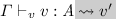
Values. Constraint generation for values takes the form . It takes as inputs a set of wanted constraints $\mathcal {Q}$, a typing environment $\varGamma$, and a ImpEff value v, and produces a value type $A$, a new set of wanted constraints $\mathcal {Q}'$, a substitution $\sigma$, and a ExEff value $v'$.

Unlike standard HM, our inference algorithm does not keep constraint generation and solving separate. Instead, the two are interleaved, as indicated by the additional arguments of our relation: (a) constraints $\mathcal {Q}$ are passed around in a stateful manner (i.e., they are input and output), and (b) substitutions $\sigma$ generated from constraint solving constitute part of the relation output. We discuss the reason for this interleaved approach in Sect. 5.4; we now focus on the algorithm.

The rules are syntax-directed on the input ImpEff value. The first rule handles term variables x: as usual for constraint-based type inference the rule instantiates the polymorphic type $(\forall \bar{\varsigma }. \overline{\alpha :\tau }. \forall \bar{\delta }. \bar{\pi } \Rightarrow A )$ of x with fresh variables; these are placeholders that are determined during constraint solving. Moreover, the rule extends the wanted constraints $\mathcal {P}$ with $\bar{\pi }$, appropriately instantiated. In ExEff, this corresponds to explicit skeleton, type, dirt, and coercion applications.

More interesting is the third rule, for term abstractions. Like in standard Hindley-Damas-Milner [5], it generates a fresh type variable $\alpha$ for the type of the abstracted term variable x. In addition, it generates a fresh skeleton variable $\varsigma$, to capture the (yet unknown) shape of $\alpha$.

As explained in detail in Sect. 5.3, the constraint solver instantiates type variables only through their skeletons annotations. Because we want to allow local constraint solving for the body c of the term abstraction the opportunity to produce a substitution $\sigma$ that instantiates $\alpha$, we have to pass in the annotation constraint $\alpha : \varsigma$.⁶ We apply the resulting substitution $\sigma$ to the result type $\sigma (\alpha ) \rightarrow \underline{ C }$.⁷

Finally, the fourth rule is concerned with handlers. Since it is the most complex of the rules, we discuss each of its premises separately:

Firstly, we infer a type $B _r\,!\,\varDelta _r$ for the right hand side of the $\mathtt {return}$-clause. Since $\alpha _r$ is a fresh unification variable, just like for term abstraction we require $\alpha _r : \varsigma _r$, for a fresh skeleton variable $\varsigma _r$.

Secondly, we check every operation clause in $\mathcal {O}$ in order. For each clause, we generate fresh skeleton, type, and dirt variables ($\varsigma _i$, $\alpha _i$, and $\delta _i$), to account for the (yet unknown) result type $\alpha _i\,!\,\delta _i$ of the continuation k, while inferring type $B _{\mathtt {Op}_i}\,!\,\varDelta _{\mathtt {Op}_i}$ for the right-hand-side $c_{\mathtt {Op}_i}$.

More interesting is the (final) set of wanted constraints $\mathcal {Q}'$. First, we assign to the handler the overall type

$$ \alpha _{in}\,!\,\delta _{in} \Rrightarrow \alpha _{out}\,!\,\delta _{out} $$

where $\varsigma _{in}, \alpha _{in}, \delta _{in}, \varsigma _{out}, \alpha _{out}, \delta _{out}$ are fresh variables of the respective sorts. In turn, we require that (a) the type of the return clause is a subtype of $\alpha _{out}\,!\,\delta _{out}$ (given by the combination of $\omega _1$ and $\omega _2$), (b) the right-hand-side type of each operation clause is a subtype of the overall result type: $\sigma ^n( B _{\mathtt {Op}_i}\,!\, \varDelta _{\mathtt {Op}_i}) \leqslant \alpha _{out}\,!\,\delta _{out}$ (witnessed by $\omega _{3_i}\,!\,\omega _{4_i}$), (c) the actual types of the continuations $B _i \rightarrow \alpha _{out}\,!\,\delta _{out}$ in the operation clauses should be subtypes of their assumed types $B _i \rightarrow \sigma ^n(\alpha _i\,!\,\delta _i)$ (witnessed by $\omega _{5_i}$). (d) the overall argument type $\alpha _{in}$ is a subtype of the assumed type of x: $\sigma ^n(\sigma _r(\alpha _r))$ (witnessed by $\omega _6$), and (e) the input dirt set $\delta _{in}$ is a subtype of the resulting dirt set $\delta _{out}$, extended with the handled operations $\mathcal {O}$ (witnessed by $\omega _7$).

All the aforementioned implicit subtyping relations become explicit in the elaborated term $c_{res}$, via explicit casts.

Fig. 9.

Constraint Generation with Elaboration (Computations)

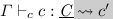
Computations. The judgement generates constraints for computations.

The first rule handles term applications of the form $v_1\,v_2$. After inferring a type for each subterm ($A _1$ for $v_1$ and $A _2$ for $v_2$), we generate the wanted constraint $\sigma _2( A _1) \leqslant A _2 \rightarrow \alpha \,!\,\delta$, with fresh type and dirt variables $\alpha$ and $\delta$, respectively. Associated coercion variable $\omega$ is then used in the elaborated term to explicitly (up)cast $v_1'$ to the expected type $A _2 \rightarrow \alpha \,!\,\delta$.

The third rule handles polymorphic let-bindings. First, we infer a type $A$ for v, as well as wanted constraints $\mathcal {Q}_v$. Then, we simplify wanted constraints $\mathcal {Q}_v$ by means of function $\mathtt {solve}$ (which we explain in detail in Sect. 5.3 below), obtaining a substitution $\sigma _1'$ and a set of residual constraints $\mathcal {Q}_v'$.

Generalization of x’s type is performed by auxiliary function $split$, given by the following clause:

In essence, $split$ generates the type (scheme) of x in parts. Additionally, it computes the subset $\mathcal {Q}_2$ of the input constraints $\mathcal {Q}$ that do not depend on locally-bound variables. Such constraints can be floated “upwards”, and are passed as input when inferring a type for c. The remainder of the rule is self-explanatory.

The fourth rule handles operation calls. Observe that in the elaborated term, we upcast the inferred type to match the expected type in the signature.

The fifth rule handles sequences. The requirement that all computations in a $\mathtt {do}$-construct have the same dirt set is expressed in the wanted constraints $\sigma _2(\varDelta _1) \leqslant \delta$ and $\varDelta _2 \leqslant \delta$ (where $\delta$ is a fresh dirt variable; the resulting dirt set), witnessed by coercion variables $\omega _1$ and $\omega _2$. Both coercion variables are used in the elaborated term to upcast $c_1$ and $c_2$, such that both draw effects from the same dirt set $\delta$.

Finally, the sixth rule is concerned with effect handling. After inferring type $A _1$ for the handler v, we require that it takes the form of a handler type, witnessed by coercion variable $\omega _1 : \sigma _2( A _1) \leqslant (\alpha _1\,!\,\delta _1 \Rrightarrow \alpha _2\,!\,\delta _2)$, for fresh $\alpha _1, \alpha _2, \delta _1, \delta _2$. To ensure that the type $A _2\,!\,\varDelta _2$ of c matches the expected type, we require that $A _2\,!\,\varDelta _2 \leqslant \alpha _1\,!\,\delta _1$. Our syntax does not include coercion variables for computation subtyping; we achieve the same effect by combining $\omega _2 : A _2 \leqslant \alpha _1$ and $\omega _3 : \varDelta _2 \leqslant \delta _1$.

Theorem 3

(Soundness of Inference). If then for any $\sigma '\,\models \,\mathcal {Q}$, we have , and analogously for computations.

Theorem 4

(Completeness of Inference). If then we have and there exists $\sigma '\,\models \,\mathcal {Q}$ and $\gamma$, such that $\sigma '(v'') = v'$ and . An analogous statement holds for computations.

5.3 Constraint Solving

The second phase of our inference-and-elaboration algorithm is the constraint solver. It is defined by the $\mathtt {solve}$ function signature:

It takes three inputs: the substitution $\sigma$ accumulated so far, a list of already processed constraints $\mathcal {P}$, and a queue of still to be processed constraints $\mathcal {Q}$. There are two outputs: the substitution $\sigma '$ that solves the constraints and the residual constraints $\mathcal {P}'$. The substitutions $\sigma$ and $\sigma '$ contain four kinds of mappings: $\varsigma \mapsto \tau$, $\alpha \mapsto A$, $\delta \mapsto \varDelta$ and $\omega \rightarrow \gamma$ which instantiate respectively skeleton variables, type variables, dirt variables and coercion variables.

Theorem 5

(Correctness of Solving). For any set $\mathcal {Q}$, the call $\mathtt {solve}(\bullet ; \bullet ; \mathcal {Q})$ either results in a failure, in which case $\mathcal {Q}$ has no solutions, or returns $(\sigma , \mathcal {P})$ such that for any $\sigma '\,\models \,\mathcal {Q}$, there exists $\sigma ''\,\models \,\mathcal {P}$ such that $\sigma ' = \sigma '' \cdot \sigma$.

The solver is invoked with $\mathtt {solve}(\bullet ;\, \bullet ;\, \mathcal {Q})$, to process the constraints $\mathcal {Q}$ generated in the first phase of the algorithm, i.e., with an empty substitution and no processed constraints. The $\mathtt {solve}$ function is defined by case analysis on the queue.

Empty Queue. When the queue is empty, all constraints have been processed. What remains are the residual constraints and the solving substitution $\sigma$, which are both returned as the result of the solver.

Skeleton Equalities. The next set of cases we consider are those where the queue is non-empty and its first element is an equality between skeletons $\tau _1 = \tau _2$. We consider seven possible cases based on the structure of $\tau _1$ and $\tau _2$ that together essentially implement conventional unification as used in Hindley-Milner type inference [5].

The first case applies when both skeletons are the same type variable $\varsigma$. Then the equality trivially holds. Hence we drop it and proceed with solving the remaining constraints. The next two cases apply when either $\tau _1$ or $\tau _2$ is a skeleton variable $\varsigma$. If the occurs check fails, there is no finite solution and the algorithm signals failure. Otherwise, the constraint is solved by instantiating the $\varsigma$. This additional substitution is accumulated and applied to all other constraints $\mathcal {P},\mathcal {Q}$. Because the substitution might have modified some of the already processed constraints $\mathcal {P}$, we have to revisit them. Hence, they are all pushed back onto the queue, which is processed recursively.

The next three cases consider three different ways in which the two skeletons can have the same instantiated top-level structure. In those cases the equality is decomposed into equalities on the subterms, which are pushed onto the queue and processed recursively.

The last catch-all case deals with all ways in which the two skeletons can be instantiated to different structures. Then there is no solution.

Skeleton Annotations. The next four cases consider a skeleton annotation $\alpha : \tau$ at the head of the queue, and propagate the skeleton instantiation to the type variable. The first case, where the skeleton is a variable $\varsigma$, has nothing to do, moves the annotation to the processed constraints and proceeds with the remainder of the queue. In the other three cases, the skeleton is instantiated and the solver instantiates the type variable with the corresponding structure, introducing fresh variables for any subterms. The instantiating substitution is accumulated and applied to the remaining constraints, which are processed recursively.

Value Type Subtyping. Next are the cases where a subtyping constraint between two value types $A _1 \leqslant A _2$, with as evidence the coercion variable $\omega$, is at the head of the queue. We consider six different situations.

If the two types are equal, the subtyping holds trivially through reflexivity. The solver thus drops the constraint and instantiates $\omega$ with the reflexivity coercion $\langle { T } \rangle$. Note that each coercion variable only appears in one constraint. So we only accumulate the substitution and do not have to apply it to the other constraints. In the next two cases, one of the two types is a type variable $\alpha$. Then we move the constraint to the processed set. We also add an equality constraint between the skeletons⁸ to the queue. This enforces the invariant that only types with the same skeleton are compared. Through the skeleton equality the type structure (if any) from the type is also transferred to the type variable. The next two cases concern two types with the same top-level instantiation. The solver then decomposes the constraint into constraints on the corresponding subterms and appropriately relates the evidence of the old constraint to the new ones. The final case catches all situations where the two types are instantiated with a different structure and thus there is no solution.

Auxiliary function $skeleton ({ A })$ computes the skeleton of $A$.

Dirt Subtyping. The final six cases deal with subtyping constraints between dirts.

If the two dirts are of the general form $\mathcal {O}\cup \delta$ and $\mathcal {O}' \cup \delta '$, we distinguish two subcases. Firstly, if $\mathcal {O}$ is empty, there is nothing to be done and we move the constraint to the processed set. Secondly, if $\mathcal {O}$ is non-empty, we partially instantiate $\delta '$ with any of the operations that appear in $\mathcal {O}$ but not in $\mathcal {O}'$. We then drop $\mathcal {O}$ from the constraint, and, after substitution, proceed with processing all constraints. For instance, for $\{ \mathtt {Op}_1 \} \cup \delta \leqslant \{ \mathtt {Op}_2 \} \cup \delta '$, we instantiate $\delta '$ to $\{ \mathtt {Op}_1 \} \cup \delta ''$—where $\delta ''$ is a fresh dirt variable—and proceed with the simplified constraint $\delta \leqslant \{ \mathtt {Op}_1, \mathtt {Op}_2 \} \cup \delta ''$. Note that due to the set semantics of dirts, it is not valid to simplify the above constraint to $\delta \leqslant \{ \mathtt {Op}_2 \} \cup \delta ''$. After all the substitution $[\delta \mapsto \{ \mathtt {Op}_1 \}, \delta '' \mapsto \emptyset ]$ solves the former and the original constraint, but not the latter.

Fig. 10.

SkelEff Syntax

The second case, $\emptyset \leqslant \varDelta '$, always holds and is discharged by instantiating $\omega$ to $\emptyset _{\varDelta '}$. The third case, $\delta \leqslant \emptyset$, has only one solution: $\delta \mapsto \emptyset$ with coercion $\emptyset _\emptyset$. The fourth case, $\mathcal {O}\cup \delta \leqslant \mathcal {O}'$, has as many solutions as there are subsets of $\mathcal {O}'$, provided that $\mathcal {O}\subseteq \mathcal {O}'$. We then simplify the constraint to $\delta \leqslant \mathcal {O}'$, which we move to the set of processed constraints. The fifth case, $\mathcal {O}\leqslant \mathcal {O}'$, holds iff $\mathcal {O}\subseteq \mathcal {O}'$. The last case, $\mathcal {O}\leqslant \mathcal {O}' \cup \delta '$, is like the first, but without a dirt variable in the left-hand side. We can satisfy it in a similar fashion, by partially instantiating $\delta '$ with $(\mathcal {O}\setminus \mathcal {O}') \cup \delta ''$—where $\delta ''$ is a fresh dirt variable. Now the constraint is satisfied and can be discarded.

5.4 Discussion

At first glance, the constraint generation algorithm of Sect. 5.2 might seem needlessly complex, due to eager constraint solving for let-generalization. Yet, we want to generalize at local $\mathtt {let}$-bound values over both type and skeleton variables,⁹ which means that we must solve all equations between skeletons before generalizing. In turn, since skeleton constraints are generated when solving subtyping constraints (Sect. 5.3), all skeleton annotations should be available during constraint solving. This can not be achieved unless the generated constraints are propagated statefully.

6 Erasure of Effect Information from ExEff

6.1 The SkelEff Language

The target of the erasure is SkelEff, which is essentially a copy of ExEff from which all effect information $\varDelta$, type information $T$ and coercions $\gamma$ have been removed. Instead, skeletons $\tau$ play the role of plain types. Thus, SkelEff is essentially System F extended with term-level (but not type-level) support for algebraic effects. Figure 10 defines the syntax of SkelEff. The type system and operational semantics of SkelEff follow from those of ExEff.

Fig. 11.

Definition of type erasure.

Discussion. The main point of SkelEff is to show that we can erase the effects and subtyping from ExEff to obtain types that are compatible with a System F-like language. At the term-level SkelEff also resembles a subset of Multicore OCaml [6], which provides native support for algebraic effects and handlers but features no explicit polymorphism. Moreover, SkelEff can also serve as a staging area for further elaboration into System F-like languages without support for algebraic effects and handlers (e.g., Haskell or regular OCaml). In those cases, computation terms can be compiled to one of the known encodings in the literature, such as a free monad representation [10, 22], with delimited control [11], or using continuation-passing style [13], while values can typically be carried over as they are.

6.2 Erasure

Figure 11 defines erasure functions $\epsilon ^{\sigma }_{\mathrm {v}}(v)$, $\epsilon ^{\sigma }_{\mathrm {c}}(c)$, $\epsilon ^{\sigma }_{\mathrm {V}}( T )$, $\epsilon ^{\sigma }_{\mathrm {C}}(\underline{ C })$ and $\epsilon ^{\sigma }_{\mathrm {E}}(\varGamma )$ for values, computations, value types, computation types, and type environments respectively. All five functions take a substitution $\sigma$ from the free type variables $\alpha$ to their skeleton $\tau$ as an additional parameter.

Thanks to the skeleton-based design of ExEff, erasure is straightforward. All types are erased to their skeletons, dropping quantifiers for type variables and all occurrences of dirt sets. Moreover, coercions are dropped from values and computations. Finally, all binders and elimination forms for type variables, dirt set variables and coercions are dropped from values and type environments.

The expected theorems hold. Firstly, types are preserved by erasure.¹⁰

Theorem 6

(Type Preservation). If ${\varGamma } \vdash _{{\scriptscriptstyle \mathtt {v}}} {v} : { T }$ then ${\epsilon ^{\emptyset }_{\mathrm {E}}(\varGamma )} \vdash _{{\scriptscriptstyle \mathtt {ev}}} {\epsilon ^{\varGamma }_{\mathrm {v}}(v)} : {\epsilon ^{\varGamma }_{\mathrm {V}}( T )}$. If ${\varGamma } \vdash _{{\scriptscriptstyle \mathtt {c}}} {c} : {\underline{ C }}$ then ${\epsilon ^{\emptyset }_{\mathrm {E}}(\varGamma )} \vdash _{{\scriptscriptstyle \mathtt {ec}}} {\epsilon ^{\varGamma }_{\mathrm {c}}(c)} : {\epsilon ^{\varGamma }_{\mathrm {C}}(\underline{ C })}$.

Here we abuse of notation and use $\varGamma$ as a substitution from type variables to skeletons used by the erasure functions.

Finally, we have that erasure preserves the operational semantics.

Theorem 7

(Semantic Preservation). If ${v} \leadsto _\mathrm {v}^{} {v'}$ then ${\epsilon ^{\sigma }_{\mathrm {v}}(v)} \equiv ^{\leadsto }_\mathrm {v} {\epsilon ^{\sigma }_{\mathrm {v}}(v')}$. If ${c} \leadsto _\mathrm {c}^{} {c'}$ then ${\epsilon ^{\sigma }_{\mathrm {c}}(c)} \equiv ^{\leadsto }_\mathrm {c} {\epsilon ^{\sigma }_{\mathrm {c}}(c')}$.

In both cases, $\equiv ^{\leadsto }$ denotes the congruence closure of the step relation in SkelEff. The choice of substitution $\sigma$ does not matter as types do not affect the behaviour.

Discussion. Typically, when type information is erased from call-by-value languages, type binders are erased by replacing them with other (dummy) binders. For instance, the expected definition of erasure would be:

$$\begin{aligned} \epsilon ^{\sigma }_{\mathrm {v}}(\varLambda (\alpha :\tau ).v) = \lambda (x:\mathtt {Unit}). \epsilon ^{\sigma }_{\mathrm {v}}(v) \end{aligned}$$

This replacement is motivated by a desire to preserve the behaviour of the typed terms. By dropping binders, values might be turned into computations that trigger their side-effects immediately, rather than at the later point where the original binder was eliminated. However, there is no call for this circumspect approach in our setting, as our grammatical partition of terms in values (without side-effects) and computations (with side-effects) guarantees that this problem cannot happen when we erase values to values and computations to computations.

7 Related Work and Conclusion

Eff’s Implicit Type System. The most closely related work is that of Pretnar [20] on inferring algebraic effects for Eff, which is the basis for our implicitly-typed ImpEff calculus, its type system and the type inference algorithm. There are three major differences with Pretnar’s inference algorithm.

Firstly, our work introduces an explicitly-typed calculus. For this reason we have extended the constraint generation phase with the elaboration into ExEff and the constraint solving phase with the construction of coercions.

Secondly, we add skeletons to guarantee erasure. Skeletons also allow us to use standard occurs-check during unification. In contrast, unification in Pretnar’s algorithm is inspired by Simonet [24] and performs the occurs-check up to the equivalence closure of the subtyping relation. In order to maintain invariants, all variables in an equivalence class (also called a skeleton) must be instantiated simultaneously, whereas we can process one constraint at a time. As these classes turn out to be surrogates for the underlying skeleton types, we have decided to keep the name.

Finally, Pretnar incorporates garbage collection of constraints [19]. The aim of this approach is to obtain unique and simple type schemes by eliminating redundant constraints. Garbage collection is not suitable for our use as type variables and coercions witnessing subtyping constraints cannot simply be dropped, but must be instantiated in a suitable manner, which cannot be done in general.

Consider for instance a situation with type variables $\alpha _1$, $\alpha _2$, $\alpha _3$, $\alpha _4$, and $\alpha _5$ where $\alpha _1 \leqslant \alpha _3$, $\alpha _2 \leqslant \alpha _3$, $\alpha _3 \leqslant \alpha _4$, and $\alpha _3 \leqslant \alpha _5$. Suppose that $\alpha _3$ does not appear in the type. Then garbage collection would eliminate it and replace the constraints by $\alpha _1 \leqslant \alpha _4$, $\alpha _2 \leqslant \alpha _4$, $\alpha _1 \leqslant \alpha _5$, and $\alpha _2 \leqslant \alpha _5$. While garbage collection guarantees that for any ground instantiation of the remaining type variables, there exists a valid ground instantiation for $\alpha _3$, ExEff would need to be extended with joins (or meets) to express a generically valid instantiation like $\alpha _1 \sqcup \alpha _2$. Moreover, we would need additional coercion formers to establish $\alpha _1 \leqslant (\alpha _1 \sqcup \alpha _2)$ or $(\alpha _1 \sqcup \alpha _2) \leqslant \alpha _4$.

As these additional constructs considerably complicate the calculus, we propose a simpler solution. We use ExEff as it is for internal purposes, but display types to programmers in their garbage-collected form.

Calculi with Explicit Coercions. The notion of explicit coercions is not new; Mitchell [15] introduced the idea of inserting coercions during type inference for ML-based languages, as a means for explicit casting between different numeric types.

Breazu-Tannen et al. [3] also present a translation of languages with inheritance polymorphism into System F, extended with coercions. Although their coercion combinators are very similar to our coercion forms, they do not include inversion forms, which are crucial for the proof of type safety for our system. Moreover, Breazu-Tannen et al.’s coercions are terms, and thus can not be erased.

Much closer to ExEff is Crary’s coercion calculus for inclusive subtyping [4], from which we borrowed the stratification of value results. Crary’s system supports neither coercion abstraction nor coercion inversion forms.

System F$_\text {C}$  [25] uses explicit type-equality coercions to encode complex language features (e.g. GADTs [16] or type families [23]). Though ExEff’s coercions are proofs of subtyping rather than type equality, our system has a lot in common with it, including the inversion coercion forms and the “push” rules.

Future Work. Our plans focus on resuming the postponed work on efficient compilation of handlers. First, we intend to adjust program transformations to the explicit type information. We hope that this will not only make the optimizer more robust, but also expose new optimization opportunities. Next, we plan to write compilers to both Multicore OCaml and standard OCaml, though for the latter, we must first adapt the notion of erasure to a target calculus without algebraic effect handlers. Finally, once the compiler shows promising preliminary results, we plan to extend it to other Eff features such as user-defined types or recursion, allowing us to benchmark it on more realistic programs.

References

Barendregt, H.: The Lambda Calculus: Its Syntax and Semantics. Studies in Logic and the Foundations of Mathematics, vol. 3. North-Holland, Amsterdam (1981)
Bauer, A., Pretnar, M.: Programming with algebraic effects and handlers. J. Logic Algebraic Program. 84(1), 108–123 (2015)
Breazu-Tannen, V., Coquand, T., Gunter, C.A., Scedrov, A.: Inheritance as implicit coercion. Inf. Comput. 93, 172–221 (1991)
Crary, K.: Typed compilation of inclusive subtyping. In: Proceedings of the Fifth ACM SIGPLAN International Conference on Functional Programming, ICFP 2000, pp, 68–81. ACM, New York (2000)
Damas, L., Milner, R.: Principal type-schemes for functional programs. In: Proceedings of the 9th ACM SIGPLAN-SIGACT Symposium on Principles of Programming Languages, POPL 1982, pp. 207–212. ACM, New York (1982)
Dolan, S., White, L., Sivaramakrishnan, K., Yallop, J., Madhavapeddy, A.: Effective concurrency through algebraic effects. In: OCaml Workshop (2015)
Girard, J.-Y., Taylor, P., Lafont, Y.: Proofs and Types. Cambridge University Press, Cambridge (1989)
Hillerström, D., Lindley, S.: Liberating effects with rows and handlers. In: Chapman, J., Swierstra, W. (eds.) Proceedings of the 1st International Workshop on Type-Driven Development, TyDe@ICFP 2016, Nara, Japan, 18 September 2016, pp. 15–27. ACM (2016)
Jones, M.P.: A theory of qualified types. In: Krieg-Brückner, B. (ed.) ESOP 1992. LNCS, vol. 582, pp. 287–306. Springer, Heidelberg (1992). https://doi.org/10.1007/3-540-55253-7_17
Kammar, O., Lindley, S., Oury, N.: Handlers in action. In: Proceedings of the 18th ACM SIGPLAN International Conference on Functional programming, ICFP 2014, pp. 145–158. ACM (2013)
Kiselyov, O., Sivaramakrishnan, K.: Eff directly in OCaml. In: OCaml Workshop (2016)
Leijen, D.: Koka: programming with row polymorphic effect types. In: Levy, P., Krishnaswami, N. (eds.) Proceedings of 5th Workshop on Mathematically Structured Functional Programming, MSFP@ETAPS 2014, Grenoble, France, 12 April 2014. EPTCS, vol. 153, pp. 100–126 (2014)
Leijen, D.: Type directed compilation of row-typed algebraic effects. In: Castagna, G., Gordon, A.D. (eds.) Proceedings of the 44th ACM SIGPLAN Symposium on Principles of Programming Languages, POPL 2017, Paris, France, 18–20 January 2017, pp. 486–499. ACM (2017)
Lindley, S., McBride, C., McLaughlin, C.: Do be do be do. In: Castagna, G., Gordon, A.D. (eds.) Proceedings of the 44th ACM SIGPLAN Symposium on Principles of Programming Languages, POPL 2017, Paris, France, 18–20 January 2017, pp. 500–514. ACM (2017). http://dl.acm.org/citation.cfm?id=3009897
Mitchell, J.C.: Coercion and type inference. In: Proceedings of the 11th ACM SIGACT-SIGPLAN Symposium on Principles of Programming Languages, POPL 1984, pp. 175–185. ACM, New York (1984)
Peyton Jones, S., Vytiniotis, D., Weirich, S., Washburn, G.: Simple unification-based type inference for GADTs. In: ICFP 2006 (2006)
Plotkin, G.D., Power, J.: Algebraic operations and generic effects. Appl. Categ. Struct. 11(1), 69–94 (2003)
Plotkin, G.D., Pretnar, M.: Handling algebraic effects. Log. Methods Comput. Sci. 9(4) (2013)
Pottier, F.: Simplifying subtyping constraints: a theory. Inf. Comput. 170(2), 153–183 (2001). https://doi.org/10.1006/inco.2001.2963
Pretnar, M.: Inferring algebraic effects. Log. Methods Comput. Sci. 10(3) (2014)
Pretnar, M.: An introduction to algebraic effects and handlers, invited tutorial. Electron. Notes Theoret. Comput. Sci. 319, 19–35 (2015)
Pretnar, M., Saleh, A.H., Faes, A., Schrijvers, T.: Efficient compilation of algebraic effects and handlers. Technical report CW 708, KU Leuven Department of Computer Science (2017)
Schrijvers, T., Peyton Jones, S., Chakravarty, M., Sulzmann, M.: Type checking with open type functions. In: ICFP 2008, pp. 51–62. ACM (2008)
Simonet, V.: Type inference with structural subtyping: a faithful formalization of an efficient constraint solver. In: Ohori, A. (ed.) APLAS 2003. LNCS, vol. 2895, pp. 283–302. Springer, Heidelberg (2003). https://doi.org/10.1007/978-3-540-40018-9_19
Sulzmann, M., Chakravarty, M.M.T., Peyton Jones, S., Donnelly, K.: System F with type equality coercions. In: Proceedings of the 2007 ACM SIGPLAN International Workshop on Types in Languages Design and Implementation, TLDI 2007, pp. 53–66. ACM, New York (2007)
Wansbrough, K., Peyton Jones, S.L.: Once upon a polymorphic type. In: POPL, pp. 15–28. ACM (1999)
Acknowledgements
We would like to thank the anonymous reviewers for careful reading and insightful comments. Part of this work is funded by the Flemish Fund for Scientific Research (FWO). This material is based upon work supported by the Air Force Office of Scientific Research under award number FA9550-17-1-0326.
Author information
Authors and Affiliations
Corresponding author
Editor information
Editors and Affiliations
Rights and permissions
Open Access This chapter is licensed under the terms of the Creative Commons Attribution 4.0 International License (http://creativecommons.org/licenses/by/4.0/), which permits use, sharing, adaptation, distribution and reproduction in any medium or format, as long as you give appropriate credit to the original author(s) and the source, provide a link to the Creative Commons license and indicate if changes were made. The images or other third party material in this book are included in the book's Creative Commons license, unless indicated otherwise in a credit line to the material. If material is not included in the book's Creative Commons license and your intended use is not permitted by statutory regulation or exceeds the permitted use, you will need to obtain permission directly from the copyright holder.
Copyright information
© 2018 The Author(s)
About this paper
Cite this paper
Saleh, A.H., Karachalias, G., Pretnar, M., Schrijvers, T. (2018). Explicit Effect Subtyping. In: Ahmed, A. (eds) Programming Languages and Systems. ESOP 2018. Lecture Notes in Computer Science(), vol 10801. Springer, Cham. https://doi.org/10.1007/978-3-319-89884-1_12
Download citation
DOI: https://doi.org/10.1007/978-3-319-89884-1_12
Published:
Publisher Name: Springer, Cham
Print ISBN: 978-3-319-89883-4
Online ISBN: 978-3-319-89884-1
eBook Packages: Computer ScienceComputer Science (R0)