WQO Dichotomy for 3-Graphs

Abstract

We investigate data-enriched models, like Petri nets with data, where executability of a transition is conditioned by a relation between data values involved. Decidability status of various decision problems in such models may depend on the structure of data domain. According to the WQO Dichotomy Conjecture, if a data domain is homogeneous then it either exhibits a well quasi-order (in which case decidability follows by standard arguments), or essentially all the decision problems are undecidable for Petri nets over that data domain.

We confirm the conjecture for data domains being 3-graphs (graphs with 2-colored edges). On the technical level, this results is a significant step beyond known classification results for homogeneous structures.

S. Lasota—Partially supported by the European Research Council (ERC) project Lipa under the EU Horizon 2020 research and innovation programme (grant agreement No. 683080).

R. Piórkowski—Partially supported by the Polish NCN grant 2016/21/B/ST6/01505.

1 Introduction

In Petri nets with data, tokens carry values from some data domain, and executability of transitions is conditioned by a relation between data values involved. One can consider unordered data, like in [25], i.e., an infinite data domain with the equality as the only relation; or ordered data, like in [21], i.e., an infinite densely totally ordered data domain; or timed data, like in timed Petri nets [1] and timed-arc Petri nets [15]. In [19] an abstract setting of Petri nets with an arbitrary fixed data domain ${\mathbb {A}}$ has been introduced, parametric in a relational structure ${\mathbb {A}}$. The setting uniformly subsumes unordered, ordered and timed data (represented by ${\mathbb {A}}= ({\mathbb {N}}, =)$, ${\mathbb {A}}= ({\mathbb {Q}}, \le )$ and ${\mathbb {A}}= ({\mathbb {Q}}, \le , +1)$, respectively).

Following [19], in order to enable finite presentation of Petri nets with data, and in particular to consider such models as input to algorithms, we restrict to relational structures ${\mathbb {A}}$ that are homogeneous [23] and effective (the formal definitions are given in Sect. 2). Certain standard decision problems (like the termination problem, the boundedness problem, or the coverability problem, jointly called from now on standard problems) are all decidable for Petri nets with ordered data [21] (and in consequence also for Petri nets with unordered data), as the model fits into the framework of well-structured transition systems of [11]. Most importantly, the structure ${\mathbb {A}}= ({\mathbb {Q}}, \le )$ of ordered data admits well quasi-order (wqo) in the following sense: for any wqo X, the set of finite induced substructures of $({\mathbb {Q}}, \le )$ (i.e., finite total orders) labeled by elements of X, ordered naturally by embedding, is a wqo (this is exactly Higman’s lemma). Moreover, essentially the same argument can be used for any other homogeneous effective data domain which admits wqo (see [19] for details). On the other hand, for certain homogeneous effective data domains ${\mathbb {A}}$ the standard problems become all undecidable. In the quest for understanding the decidability borderline, the following hypothesis has been formulated in [19]:

Conjecture 1

(Wqo Dichotomy Coinjecture [19]). For an effective homogeneous structure ${\mathbb {A}}$, either ${\mathbb {A}}$ admits wqo (in which case the standard problems are decidable for Petri nets with data ${\mathbb {A}}$), or all the standard problems are undecidable for Petri nets with data ${\mathbb {A}}$.

According to [19], the conjecture could have been equivalently stated for another data-enriched models, e.g., for finite automata with one register [2]. In this paper we consider, for the sake of presentation, only Petri nets with data. Wqo Dichotomy Conjecture holds in special cases when data domains ${\mathbb {A}}$ are undirected or directed graphs, due to the known classifications of homogeneous graphs [6, 18].

Contributions. We confirm the Wqo Dichotomy Conjecture for data domains ${\mathbb {A}}$ being strongly¹ homogeneous 3-graphs. A 3-graph is a logical structure with three irreflexive symmetric binary relations such that every pair of elements of ${\mathbb {A}}$ belongs to exactly one of the relations (essentially, a clique with 3-colored edges).

Our main technical contribution is a complex analysis of possible shapes of strongly homogeneous 3-graphs, constituting the heart of the proof. We believe that this is a significant step towards full classification of homogeneous 3-graphs. The classification of homogeneous structures is a well-known challenge in model theory, and has been only solved in some cases by now: for undirected graphs [18], directed graphs (the proof of Cherlin spans a book [6]), multi-partite graphs [16], and few others (the survey [23] is an excellent overview of homogeneous structures). Although the full classification of homogeneous 3-graphs was not our primary objective, we believe that our analysis significantly improves our understanding of these structures and can be helpful for classification.

Our result does not fully settle the status of the Wqo Dichotomy Conjecture. Dropping the (mild) strong homogeneity assumption, as well as extending the proof to arbitrarily many symmetric binary relations, is left for future work.

Related Research. Net models similar to Petri nets with data have been continuously proposed since the 80s, including, among the others, high-level Petri nets [13], colored Petri nets [17], unordered and ordered data nets [21], $\nu$-Petri nets [25], and constraint multiset rewriting [5, 8, 9]. Petri nets with data can be also considered as a reinterpretation of the classical definition of Petri nets in sets with atoms [3, 4], where one allows for orbit-finite sets of places and transitions instead of just finite ones. The decidability and complexity of standard problems for Petri nets over various data domains has attracted a lot of attention recently, see for instance [14, 21, 22, 24, 25].

Wqos are important for their wide applicability in many areas. Studies of wqos similar to ours, in case of graphs, have been conducted by Ding [10] and Cherlin [7]; their framework is different though, as they concentrate on subgraph ordering while we investigate induced subgraph (or substructure) ordering.

2 Petri Nets with Homogeneous Data

In this section we provide all necessary preliminaries. Our setting follows [19] and is parametric in the underlying logical structure ${\mathbb {A}}$, which constitutes a data domain. Here are some example data domains:

• Equality data domain: natural numbers with equality ${\mathbb {A}}_{=}= ({\mathbb {N}}, =)$. Note that any other countably infinite set could be used instead of natural numbers, as the only available relation is equality.

• Total order data domain: rational numbers with the standard order ${\mathbb {A}}_{\le }= ({\mathbb {Q}}, \le )$. Again, any other countably infinite dense total order without extremal elements could be used instead.

• Nested equality data domain: ${\mathbb {A}}_{1}= ({\mathbb {N}}^2, =_1, =)$ where $=_1$ is equality on the first component: $(n, m) =_1 (n', m')$ if $n = n'$ and $m\ne m'$. Essentially, ${\mathbb {A}}$ is an equivalence relation with infinitely many infinite equivalence classes.

Note that two latter structures essentially extend the first one: in each case the equality is either present explicitly, or is definable. From now on, we always assume a fixed countably infinite relational structure ${\mathbb {A}}$ with equality over a finite vocabulary (signature) $\varSigma$.

Petri Nets with Data. Petri nets with data are exactly like classical place/transition Petri nets, except that tokens carry data values and these data values must satisfy a prescribed constraint when a transition is executed. Formally, a Petri net with data ${\mathbb {A}}$ consists of two disjoint finite sets P (places) and T (transitions), the arcs $A \subseteq P{\times } T \cup T{\times } P$, and two labelings:

• arcs are labelled by pairwise disjoint finite nonempty sets of variables;

• transitions are labelled by first-order formulas over the vocabulary $\varSigma$ of ${\mathbb {A}}$, such that free variables of the formula labeling a transition t belong to the union of labels of the arcs incident to t.

Example 1

For illustration consider a Petri net with equality data ${\mathbb {A}}_{=}$, with two places $p_1, p_2$ and two transitions $t_1, t_2$ depicted on Fig. 1. Transition $t_1$ outputs two tokens with arbitrary but distinct data values onto place $p_1$. Transition $t_2$ inputs two tokens with the same data value, say a, one from $p_1$ and one from $p_2$, and outputs 3 tokens: two tokens with arbitrary but equal data values, say b, one onto $p_1$ and the other onto $p_2$; and one token with a data value $c \ne a$ onto $p_2$. Note that the transition $t_2$ does not specify whether $b=a$, or $b = c$, or $b \ne a,c$, and therefore all three options are allowed. Variables $y_1, y_2$ can be considered as input variables of $t_2$, while variables $z_1, z_2, z_3$ can be considered as output ones; analogously, $t_1$ has no input variables, and two output ones $x_1, x_2$.

Fig. 1.

A Petri net with equality data, with places $P = \{p_1, p_2\}$ and transitions $T = \{t_1, t_2\}$. In the shown configuration, $t_2$ can be fired: consume two tokens carrying 3, and put, e.g., token carrying 4 on $p_1$ and tokens carrying 4, 6 on $p_2$.

The formal semantics of Petri nets with data is given by translation to multiset rewriting. Given a set X, finite or infinite, a finite multiset over X is a finite (possibly empty) partial function from X to positive integers. In the sequel let $\mathcal{M}(X)$ stand for the set of all finite multisets over X. A multiset rewriting system $(\mathcal{{P}}, \mathcal{{T}})$ consists of a set $\mathcal{{P}}$ together with a set of rewriting rules:

$$ \mathcal{{T}}\quad \subseteq \quad \mathcal{M}(\mathcal{{P}}) \times \mathcal{M}(\mathcal{{P}}). $$

Configurations $C \in \mathcal{M}(\mathcal{{P}})$ are finite multisets over $\mathcal{{P}}$, and the step relation $\longrightarrow$ between configurations is defined as follows: for every $(I, O) \in \mathcal{{T}}$ and every $M \in \mathcal{M}(\mathcal{{P}})$, there is the step ($+$ stands for multiset union)

$$ M + I \ \longrightarrow \ M + O. $$

For instance, a classical Petri net induces a multiset rewriting system where $\mathcal{{P}}$ is the set of places, and $\mathcal{{T}}$ is essentially the set of transitions, both $\mathcal{{P}}$ and $\mathcal{{T}}$ being finite. Configurations correspond to markings.

A Petri net with data ${\mathbb {A}}$ induces a multiset rewriting system $(\mathcal{{P}}, \mathcal{{T}})$, where $\mathcal{{P}}= P \times {\mathbb {A}}$ and thus is infinite. Configurations are finite multisets over $P\times {\mathbb {A}}$ (cf. a configuration depicted in Fig. 1). The rewriting rules $\mathcal{{T}}$ are defined as

$$ \mathcal{{T}}\quad = \quad \bigcup _{t\in T} \mathcal{{T}}_t, $$

where the relation $\mathcal{{T}}_t \subseteq \mathcal{M}(\mathcal{{P}}) \times \mathcal{M}(\mathcal{{P}})$ is defined as follows: Let $\phi$ denote the formula labeling the transition t, and let $X_i$, $X_o$ be the sets of input and output variables of t. Every valuation $v_i : X_i \rightarrow {\mathbb {A}}$ gives rise to a multiset $M_{v_i}$ over $\mathcal{{P}}$, where $M_{v_i}(p, a)$ is the (positive) number of variables x labeling the arc (p, t) with $v_i(x) = a$. Likewise for valuations $v_o : X_o \rightarrow {\mathbb {A}}$. Then let

$$ \mathcal{{T}}_t = \left\{ \, (M_{v_i}, M_{v_o}) \, | \, v_i : X_i \rightarrow {\mathbb {A}}, \ v_o : X_o \rightarrow {\mathbb {A}}, \ v_i, v_o \vDash \phi \,\right\} . $$

Like $\mathcal{{P}}$, the set of rewriting rules $\mathcal{{T}}$ is infinite in general.

As usual, for a net N and its configuration C, a run of (N, C) is a maximal, finite or infinite, sequence of steps starting in C.

Remark 1

As for classical Petri nets, an essentially equivalent definition can be given in terms of vector addition systems (such a variant has been used in [14] for equality data). Petri nets with equality data are equivalent to (even if defined differently than) unordered data Petri nets of [21], and Petri nets with total ordered data are equivalent to ordered data Petri nets of [21].

Effective Homogeneous Structures. For two relational $\varSigma$-structures $\mathcal{{A}}$ and $\mathcal{{B}}$ we say that $\mathcal{{A}}$ embeds in $\mathcal{{B}}$, written $\mathcal{{A}} \unlhd \mathcal{{B}}$, if $\mathcal{{A}}$ is isomorphic to an induced substructure of $\mathcal{{B}}$, i.e., to a structure obtained by restricting $\mathcal{{B}}$ to a subset of its domain. This is witnessed by an injective function² $h : \mathcal{{A}} \rightarrow \mathcal{{B}}$, which we call embedding. We write ${\textsc {Age}}({\mathbb {A}}) = \left\{ \, \mathcal{{A}} \text { a finite structure} \, | \, \mathcal{{A}} \unlhd {\mathbb {A}}\,\right\}$ for the class of all finite structures that embed into ${\mathbb {A}}$, and call it the age of${\mathbb {A}}$.

Homogeneous structures are defined through their automorphisms: ${\mathbb {A}}$ is homogeneous if every isomorphism of two its finite induced substructures extends to an automorphism of ${\mathbb {A}}$. In the sequel we will also need an equivalent definition using amalgamation. An amalgamation instance consists of three structures $\mathcal{{A}}, \mathcal{{B}}_1, \mathcal{{B}}_2 \in {\textsc {Age}}({\mathbb {A}})$ and two embeddings $h_1 : \mathcal{{A}}\rightarrow \mathcal{{B}}_1$ and $h_2 : \mathcal{{A}} \rightarrow \mathcal{{B}}_2$. A solution of such instance is a structure $\mathcal{{C}} \in {\textsc {Age}}({\mathbb {A}})$ and two embeddings $g_1 : \mathcal{{B}}_1 \rightarrow \mathcal{{C}}$ and $g_2 : \mathcal{{B}}_2 \rightarrow \mathcal{{C}}$ such that $g_1 \circ h_1 = g_2 \circ h_2$ (we refer the reader to [12] for further details). Intuitively, $\mathcal{{C}}$ represents ‘gluing’ of $\mathcal{{B}}_1$ and $\mathcal{{B}}_2$ along the partial bijection $h_2 \circ ({h_1}^{-1})$. In this paper we will restrict ourselves to singleton amalgamation instances, where only one element of $\mathcal{{B}}_1$ is outside of $h_1(\mathcal{{A}})$, and likewise for $\mathcal{{B}}_2$.

An example singleton amalgamation instance is shown on the right, where the graph $\mathcal{{A}}$ consists of the single edge connecting two middle black nodes, $\mathcal{{B}}_1$ is the left triangle, and $\mathcal{{B}}_2$ the right one. The dashed line represents an edge that may (but does not have to) appear in a solution. ${\mathbb {A}}$ is homogeneous if, and only if every amalgamation instance has a solution; in such case we say that ${\textsc {Age}}({\mathbb {A}})$ has the amalgamation property. See [23] for further details.

A solution $\mathcal{{C}}$ necessarily satisfies $g_1(h_1(\mathcal{{A}})) = g_2(h_2(\mathcal{{A}})) \subseteq g_1(\mathcal{{B}}_1) \cap g_2(\mathcal{{B}}_2)$; a solution is strong if $g_1(h_1(\mathcal{{A}})) = g_1(\mathcal{{B}}_1) \cap g_2(\mathcal{{B}}_2)$. Intuitively, this forbids additional gluing of $\mathcal{{B}}_1$ and $\mathcal{{B}}_2$ not specified by the partial bijection $h_2 \circ ({h_1}^{-1})$. If every amalgamation instance has a strong solution we call ${\mathbb {A}}$ strongly homogeneous. This is a mild restriction, as homogeneous structures are typically strongly homogeneous.

The equality, nested equality, and total order data domains are strongly homogeneous structures. For instance, in the latter case finite induced substructures are just finite total orders, which satisfy the strong amalgamation property. Many other natural classes of structures have the amalgamation property: finite graphs, finite directed graphs, finite partial orders, finite tournaments, etc. Each of these classes is the age of a strongly homogeneous relational structure, namely the universal graph (called also random graph), the universal directed graph, the universal partial order, the universal tournament, respectively. Examples of homogeneous structures abound [23].

Homogeneous structures admit quantifier elimination: every first-order formula is equivalent to (i.e., defines the same set as) a quantifier-free one [23]. Thus it is safe to assume that formulas labeling transitions are quantifier-free.

Admitting wqo . A well quasi-order (wqo) is a well-founded quasi-order with no infinite antichains. For instance, finite multisets $\mathcal{M}(P)$ over a finite set P, ordered by multiset inclusion $\sqsubseteq$, are a wqo. Another example is the embedding quasi-order $\unlhd$ in ${\textsc {Age}}({\mathbb {A}}_{\le })$ (= all finite total orders) isomorphic to the ordering of natural numbers. Finally, the embedding quasi-order in ${\textsc {Age}}({\mathbb {A}})$ can be lifted from finite structures to finite structures labeled by elements of some ordered set $(X, \le )$: for two such labeled structures $a : \mathcal{{A}} \rightarrow X$ and $b: \mathcal{{B}} \rightarrow X$ we define $a \unlhd _{X} b$ if some embedding $h : \mathcal{{A}} \rightarrow \mathcal{{B}}$ satisfies $a(x) \le b(h(x))$ for every $x\in \mathcal{{A}}$. We say that ${\mathbb {A}}$ admits wqo when for every wqo $(X, \le )$, the lifted embedding order $\unlhd _{X}$ is a wqo too. For instance, ${\mathbb {A}}_{\le }$ admits wqo by Higman’s lemma. The Wqo Dichotomy Conjecture for homogeneous undirected (and also directed) graphs is easily shown by inspection of the classifications thereof [6, 18]:

Theorem 1

A homogeneous graph ${\mathbb {A}}$ either admits wqo, or all standard problems are undecidable for Petri nets with data ${\mathbb {A}}$.

Note the natural correspondence between configurations of a Petri net with data ${\mathbb {A}}$, and structures $\mathcal{{A}} \in {\textsc {Age}}({\mathbb {A}})$ labeled by finite multisets over the set P of places:

$$ \mathcal{M}(P \times {\mathbb {A}}) \quad \equiv \quad \left\{ \, m : \mathcal{{A}} \rightarrow \mathcal{M}(P) \, | \, \mathcal{{A}}\in {\textsc {Age}}({\mathbb {A}})\,\right\} . $$

Thus the lifted embedding quasi-order $\unlhd _{\mathcal{M}(P)}$ is an order on configurations.

Standard Decision Problems. A Petri net with data N can be finitely represented by finite sets P, T, A and appropriate labelings with variables and formulas. Due to the homogeneity of ${\mathbb {A}}$, a configuration C can be represented (up to automorphism of ${\mathbb {A}}$) by a structure $\mathcal{{A}} \in {\textsc {Age}}(A)$ labeled by $\mathcal{M}(P)$. We can thus consider the classical decision problems that input Petri nets with data ${\mathbb {A}}$, like the termination problem: does a given (N, C) have only finite runs? The data domain is considered as a parameter, and hence itself does not constitute part of input. Another classical problem is the place non-emptiness problem (markability): given (N, C) and a place p of N, does (N, C) admit a run that puts at least one token on place p? One can also define the appropriate variants of the coverability problem (equivalent to the place non-emptiness problem), the boundedness problem, the evitability problem, etc. (see [19] for details). All the decision problems mentioned above we jointly call standard problems.

A $\varSigma$-structure ${\mathbb {A}}$ is called effective if the following age problem for ${\mathbb {A}}$ is decidable: given a finite $\varSigma$-structure $\mathcal{{A}}$, decide whether $\mathcal{{A}} \unlhd {\mathbb {A}}$. If ${\mathbb {A}}$ admits wqo then application of the framework of well-structured transition systems [11] to the lifted embedding order $\unlhd _{\mathcal{M}(P)}$ yields:

Theorem 2

([19]). If an effective homogeneous structure ${\mathbb {A}}$ admits wqo then all the standard problems are decidable for Petri nets with data ${\mathbb {A}}$.

3 Results

A 3-graph ${\mathbb {G}}= (V, C_1, C_2, C_3)$ consists of a set V and three irreflexive symmetric binary relations $C_1, C_2, C_3 \subseteq V^2$ such that every pair of distinct elements of V belongs to exactly one of the three relations. In the sequel we treat a 3-graph as a clique with 3-colored edges. Any graph, including ${\mathbb {A}}_{=}$ and ${\mathbb {A}}_{1}$, can be seen as a 3-graph. Our main result confirms the Wqo Dichotomy Conjecture for strongly homogeneous 3-graphs:

Theorem 3

An effective strongly homogeneous 3-graph ${\mathbb {G}}$ either admits wqo, or all standard problems are undecidable for Petri nets with data ${\mathbb {G}}$.

The core technical result of the paper is Theorem 4 below. A path is a finite graph with nodes $\{v_1, \ldots , v_n\}$ whose only edges are pairs $\{v_i, v_{i+1}\}$. The nodes $v_1, v_n$ are ends of the path, and n is its length.

Theorem 4

A strongly homogeneous 3-graph ${\mathbb {G}}$ either admits wqo, or for some $i, j \in \{1, 2, 3\}$ (not necessarily distinct) the graph $(V, C_i \cup C_j)$ contains arbitrarily long paths as induced subgraphs.

In the rest of the paper we concentrate solely on (parts of) the proof of Theorem 4. The omitted parts, and well as the proof that Theorem 4 implies Theorem 3, are to be found in the full version of this paper [20].

Example 2

For a quasi-order $(X, \le )$, the multiset inclusion is defined as follows for $m, m' \in \mathcal{M}(X)$: $m'$ is included in m if $m'$ is obtained from m by a sequence of operations, where each operation either removes some element, or replaces some element by a smaller one wrt. $\le$. The structure ${\mathbb {A}}_{=}= ({\mathbb {N}}, =)$ admits wqo. Indeed, ${\textsc {Age}}({\mathbb {A}}_{=})$ contains just finite pure sets, thus $\unlhd _{X}$ is quasi-order-isomorphic to the multiset inclusion on $\mathcal{M}(X)$, and is therefore a wqo whenever the underlying quasi-order $(X, \le )$ is. Similarly, ${\mathbb {A}}_{1}= ({\mathbb {N}}^2, =_1, =)$ also admits wqo, as $\unlhd _{X}$ is quasi-order-isomorphic to the multiset inclusion on $\mathcal{M}(\mathcal{M}(X))$.

On the other hand, consider a 3-graph $({\mathbb {N}}^2, =_1, =_2,$ $\ne _{12})$ where $=_2$ is symmetric to $=_1$ and $(n, m) \ne _{12} (n', m')$ if $n \ne n'$ and $m \ne m'$. It refines ${\mathbb {A}}_{1}$ and does not admit wqo. Indeed, in agreement with Theorem 4, the graph $({\mathbb {N}}^2, =_1 \cup =_2)$ contains arbitrarily long paths of the shape presented on the right, where the two colors depict $=_1$ and $=_2$, respectively, and lack of color corresponds to $\ne _{12}$. Note that $({\mathbb {N}}^2, =_1, =_2, \ne _{12})$ is homogeneous but not strongly so.

4 Proof of Theorem 4

From now on we consider a fixed 3-graph ${\mathbb {G}}= (V, C_1, C_2, C_3)$ as data domain, assuming ${\mathbb {G}}$ to be countably infinite and strongly homogeneous. We treat ${\mathbb {G}}$ as a clique with 3-colored edges: we call $C_1, C_2$ and $C_3$ colors and put . To denote individual colors from this set, we will use variables and . A path in the graph we call (); for simplicity, we will write instead of -path. Likewise we speak of -cliques, -cliques, -cycles, etc. A triangle is a 3-clique with edges colored by . (Note that ).

Sketch of the Proof. The Lemma 1 below states that any 3-graph ${\mathbb {G}}$ has to meet one of the four listed cases. It splits the proof into four separate paths:

We present in detail only one of the three nontrivial paths – one corresponding to case (C). Cases (A) and (B) are treated in the full version [20]. Case (A) constitutes the most difficult part of the proof and involves a complex and delicate analysis of consequences of the amalgamation property. It consists of four step that deduce extension of the assumed induced substructures by individual vertices, individual edges, paths of length 2, resp., culminating in derivation of arbitrarily long paths. Thus in case (A) only the second condition of Theorem 4 is possible, while in the other two cases both conditions of Theorem 4 may hold true.

Lemma 1

Every homogeneous 3-graph ${\mathbb {G}}= (V, C_1, C_2, C_3)$ satisfies one of the following conditions:

• (A) for some color , ${\mathbb {G}}$ contains the following induced substructures:

  

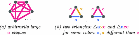
• (B) for some colors , is a union of disjoint cliques,

• (C) for some color , is a union of finitely many disjoint infinite cliques,

• (D) for some colors , contains arbitrarily long paths.

Proof

By Ramsey theorem, ${\mathbb {G}}$ contains an arbitrarily large monochromatic cliques. Let us state a bit stronger requirement:

Condition $\spadesuit$: For some , ${\mathbb {G}}$ contains arbitrarily large -cliques and a triangle with exactly two -edges ().

Consider two cases, depending on whether the condition $\spadesuit$ is satisfied or not.

Case $1^\circ$. Assume that ${\mathbb {G}}$ contains both arbitrarily large -cliques and a triangle for some . Let be the third, remaining color. Our goal will be to show that either (A) or (B) holds.

If the graph is a disjoint sum of cliques, we immediately obtain (B). Suppose the contrary. We get that ${\mathbb {G}}$ has to contain one of the three possible counterexamples for transitivity of relation :

If it contains the triangle or , case (A) holds.

Suppose we got . Let us check this time whether colors and form a union of disjoint cliques. Again, if it is so, we easily get (B), so we assume the contrary. Similarly, we necessarily obtain one of the following triangles:

This time case (A) also holds for two out of the three triangles above:

• for , because together with subgraphs resulting from assumption $\spadesuit$ (i.e. with triangle and the -cliques) we get all graphs required by (A).

• for paired with the triangle we just obtained, using color appearing in those triangles in place of in condition (A).

It only remains to consider the situation when we got . We use it together with previously obtained triangle to build the following instance of singleton amalgamation:

Depending on the color of the dashed edge, in the solution we get one of the following triangles:

and each one alone completes the requirements of (A). This closes case $1^\circ$.

Case $2^\circ$. Suppose condition $\spadesuit$ is false. Remind that ${\mathbb {G}}$ contains arbitrarily large -cliques for some . Since $\spadesuit$ does not hold, the graph does not contain a triangle – in other words, the color appears only within cliques. We conclude that is a union of disjoint cliques. Clearly at least one of such cliques has to be infinite. By homogeneity we get that all the cliques in have to be infinite. Now our target is to show that either (C) or (D) holds.

The case (C) is fulfilled when there are only finitely many -cliques. Let us assume the contrary. In each of the -cliques we chose one vertex. Edges between the chosen vertices form an infinite -clique K. Using Ramsey theorem again, we conclude that in K one of the colors forms arbitrarily large monochromatic cliques. W.l.o.g. suppose that this is color .

If the graph ${\mathbb {G}}$ contained for some , then the assumptions of $\spadesuit$ would be met, leading to a contradiction. Therefore we conclude that is a union of disjoint infinite -cliques.

When there are only finitely many -cliques, condition (C) is fulfilled. Otherwise we know that ${\mathbb {G}}$ is a union of infinitely many -cliques for both and . Using homogenity, it is easy to show that then every pair of differently colored cliques has exactly one common vertex, so the graph ${\mathbb {G}}$ takes the form as depicted in Example 2. A graph of such form contains arbitrarily long -path, so the requirements of (D) are met.    $\square$

4.1 Case (C)

Let be the color that satisfies condition (C), and , — the remaining two colors. In this section we often treat ${\mathbb {G}}$ as the k-partite graph (for some $k\in \mathbb {N}$): k cliques of color allow to distinguish k groups of vertices $V_1 \cup V_2 \cup \dots \cup V_k = V$ (from now on we will refer to them as layers). The remaining two colors can be interpreted as existence () and nonexistence () of edges between these groups.

Remark $\bigstar$: We observe that the special color between vertices within each layer $V_i$ ensures that the automorphisms of ${\mathbb {G}}$ will not ‘mix’ those layers: when two vertices u, v belong to a common layer $V_i$, then their images f(u), f(v) will also belong to some common layer $V_j$, no matter what automorphism $f \in \mathrm{Aut}({\mathbb {G}})$ we choose. Obviously, the automorphisms can switch positions of whole layers, e.g. move all vertices from $V_i$ to some $V_j$ and vice versa—in this respect the layers are undistinguishable.

Lemma 2

For every $i, j \in \{1, 2, \dots , k\}$ and () the bipartite graph (with two distinguishable sides $V_i, V_j$) is homogeneous.

The vertex sets $V_i$ and $V_j$ are used here as unary relations that allow to tell the two layers of ${\mathbb {G}}_{i,j}$ (sides of ${\mathbb {G}}_{i,j}$) apart. An example is shown on the right, with three layers $V_1, V_2$ and $V_3$, and three bipartite graphs ${\mathbb {G}}_{1,2}$, ${\mathbb {G}}_{2,3}$ and ${\mathbb {G}}_{1,3}$.

Proof

Fix ${\mathbb {G}}_{i,j}$ a bipartite graph. To prove its homogeneity we have to show that each isomorphism of two of its finite induced subgraphs may be extended to some automorphism of ${\mathbb {G}}_{i,j}$. Let us then take some given automorphism $f: G_1 \rightarrow G_2$ for some finite induced subgraphs $G_1, G_2$ of ${\mathbb {G}}_{i,j}$. It is easy to extend it to a full automorphism when it ‘touches’ both layers of $G_{i,j}$, i.e.:

$$ V(G_1) \cap V_i \ne \emptyset \,\, \wedge \,\, V(G_1) \cap V_j \ne \emptyset $$

where $V(G_1)$ is the set of vertices of $G_1$. In this case, by homogeneity of ${\mathbb {G}}$, we construct a full automorphism $f' : {\mathbb {G}}\rightarrow {\mathbb {G}}$, which extends f. It is easy to see that in this case $f'$ has to fix the layers $V_i$ and $V_j$, and hence $f'$ restricted to the graph ${\mathbb {G}}_{i,j}$ is a correct automorphism of this graph.

Things get more complicated when f operates only on some single layer of ${\mathbb {G}}_{i,j}$. W.l.o.g. suppose that it ‘touches’ only $V_i$, so $V(G_1) \cap V_j = \emptyset$. Now the above construction will not work out of the box—if we were unlucky, the automorphism of ${\mathbb {G}}$ we get by homogeneity moves the whole layer $V_j$ to some $V_n$ located ‘outside’ the graph ${\mathbb {G}}_{i,j}$ ($n \notin \{i, j\}$).

It will be handy to make the following observation: when f ‘touches’ only $V_i$ we may assume that $V(G_1) \cap V(G_2) = \emptyset$. Indeed, every function $g: G_1 \rightarrow G_2$ that violates this condition may be decomposed as $g = f_2 \circ f_1$ for some $f_1, f_2$:

$$ G_1 \xrightarrow {f_1} H \xrightarrow {f_2} G_2 $$

such that H is disjoint both with $G_1$ and with $G_2$.

Now, let $N = |V(G_1)| = |V(G_2)|$ be the size of the domain of isomorphism f. Let us take an arbitrary infinite family $(S_n)_{n \in \mathbb {N}}$ of subgraphs of ${\mathbb {G}}$ with disjoint vertex sets, such that the following conditions are met:

• $|V(S_n) \cap V_m| = 1$ for $m \ne i$ (and this single vertex will be denoted as $v_m^{(n)}$),

• $|V(S_n) \cap V_i| = N$ (denote these vertices as $s^{(n)}_1, s^{(n)}_2, s^{(n)}_3, \dots , s^{(n)}_N$).

We define a connection type of a layer $V_i$ with $V_m$ in the graph $S_n$ as the N-element sequence of colors of edges from the list bellow:

$$ (\{s^{(n)}_1, v_m^{(n)}\}, \{s^{(n)}_2, v_m^{(n)}\}, \dots , \{s^{(n)}_N, v_m^{(n)}\}) $$

E.g. in the graph bellow, the connection type of layer $V_i = V_3$ with $V_1$ is , and with $V_2$ — (remembering that is treated as lack of an edge):

Furthermore, we define the type of graph $S_n$ to be the sequence of types arising between $V_i$ and other layers plus the list of edge-colors between all pairs of vertices $v_\bullet ^{(n)}$ (enumerated in some consistent way). As there are only finitely many such types, by pigeonhole principle there exists a pair of graphs $S_a$ and $S_b$ with the same type.

Let us fix some order on vertices of $G_1$: $V(G_1) = \{g_1, g_2, \dots , g_N\}$. Let h be the partial isomorphism that moves the vertices as follows:

$$\begin{aligned} s^{(a)}_1&\rightarrow g_1&s^{(b)}_1&\rightarrow f(g_1)\\&\dots&\dots \\ s^{(a)}_N&\rightarrow g_N&s^{(b)}_N&\rightarrow f(g_N) \end{aligned}$$

By homogeneity, it has to extend to a full automorphism $h'\in \mathrm{Aut}({\mathbb {G}})$. In particular, in the neighbourhood of $G_1$ and $G_2$ there will be images of all vertices $v_\bullet ^{(\alpha )}$ of graphs $S_a$ and $S_b$:

$$ h'\!\left( v_1^{(\alpha )}\right) , h'\!\left( v_2^{(\alpha )}\right) , \ \dots , h'\!\left( v_{i-1}^{(\alpha )}\right) , h'\!\left( v_{i+1}^{(\alpha )}\right) , \ \dots , h'\!\left( v_k^{(\alpha )}\right) $$

(for $\alpha$ in $\{a, b\}$). What follows is that $G_1$ with added vertices $h'(v_\bullet ^{(a)})$ has the same type as $G_2$ with $h'(v_\bullet ^{(b)})$ respectively (that type may differ from the type of $S_a$ and $S_b$ though!). It is best illustrated on a picture:

Above, the colored triangles represent the types of connections. The order of those types may get permuted when applying $h'$, but still—in line with the remark $\bigstar$ — for each $\beta \in \{1,2,\dots , k\} \setminus \{i\}$ the vertex $h'\!\left( v_\beta ^{(a)}\right)$ must stay in the same layer as $h'\!\left( v_\beta ^{(b)}\right)$, furthermore their type of connection with layer $V_i$ is preserved.

Extending the isomorphism f in a natural way (thanks to the compatibility of types) on those newly obtained vertices:

$$ h'\left( v_\bullet ^{(a)}\right) \xrightarrow {f} h'\left( v_\bullet ^{(b)}\right) $$

we get an isomorphism that this time ‘operates’ on all layers $V_\bullet$. If we now extend it to an automorphism of the whole ${\mathbb {G}}$, we will get a function that fixes all layers $V_\bullet$. This function may be safely restricted to $V_i \cup V_j$, staying a correct automorphism of our initial bipartite graph ${\mathbb {G}}_{i,j}$, which completes the proof.    $\square$

We are going to apply to graphs ${\mathbb {G}}_{i,j}$ the following classification result:

Theorem 5

([16]). A countably infinite homogeneous bipartite graph (with distinguishable sides) is either empty, or full, or a perfect matching, or the complement of a perfect matching, or a universal graph.

From our point of view, all we need to know about the universal graph is that it contains arbitrarily long paths which – translated to our notation – would mean that ${\mathbb {G}}_{i,j}$ contains arbitrarily long -paths. Therefore in our further considerations we assume that ${\mathbb {G}}_{i,j}$ is not universal which, in our notation, leaves two types of ${\mathbb {G}}_{i,j}$:

• 1. all edges of ${\mathbb {G}}_{i, j}$ have the same color , i.e. ${\mathbb {G}}_{i,j}$ is a full or empty bipartite graph,

• 2. one of the colors forms a perfect matching in ${\mathbb {G}}_{i,j}$, the second one () is then the complement of this matching.

Graphs of type 2. may be seen as bijections between their sets of vertices (layers). Lemma 3 states that those bijections have to agree with each other.

Lemma 3

Let $V_i, V_j, V_k$ be some arbitrary pairwise different layers, such that ${\mathbb {G}}_{i, j}$ is of type 2 and $\psi : V_i \rightarrow V_j$ is the bijection it determines. Then $\psi$ takes to , or to its complement. Formally:

Proof

We head towards a contradiction. Negating the claim we get:

$$\begin{aligned} \Big ( \mathop {\exists }\limits _{u \in V_i} \mathop {\exists }\limits _{v \in V_k} \lnot \clubsuit \wedge \spadesuit&\ \ \vee \ \ \clubsuit \wedge \lnot \spadesuit \Big ) \ \wedge \ \Big ( \mathop {\exists }\limits _{u \in V_i} \mathop {\exists }\limits _{v \in V_k} \lnot \heartsuit \wedge \diamondsuit&\ \ \vee \ \ \heartsuit \wedge \lnot \diamondsuit \Big ) \end{aligned}$$

which leads to four cases with similar proofs. We will consider one of them (corresponding to $\lnot \heartsuit \wedge \diamondsuit$ and $\clubsuit \wedge \lnot \spadesuit$) and omit the other. Let us then assume that there exist $x, x' \in V_i$ and $y, y' \in V_k$ such that:

Let g be a partial isomorphism of the form $g = \{ x \rightarrow x', y \rightarrow y'\}$. By homogeneity of ${\mathbb {G}}$, there is some full automorphism $g' \in \mathrm{Aut}({\mathbb {G}})$ extending g. If additionally we were able to force g to fix the layer $V_j$, we would be almost done. Let us try to achieve that property.

For that purpose, in $V_j$ we choose a vertex v such that:

• I. $v \notin \psi (\{x, x'\})$,

• II. if ${\mathbb {G}}_{j,k}$ is a graph of type 2. defining a bijection $\phi :V_k \rightarrow V_j$, then also $v \notin \phi (\{y, y'\})$.

Clearly such vertex must exist – two above conditions exclude at most 4 different vertices from the infinite set of candidates. The function g extended with $v \xrightarrow {g} v$ stays a correct isomorphism, because:

• in ${\mathbb {G}}_{i,j}$ by definition of isomorphism we need the edges $\{x, v\}$ and $\{g(x), g(v)\}$ to be equally colored, and, in fact, they are. We get this thanks to the condition I.: x is connected with all vertices from $V_j \setminus \{\psi (x)\}$ by -edges, . We similarly handle $x'$.

• in turn in ${\mathbb {G}}_{j,k}$ — if it is a graph of type 1, the needed equality of colors of edges $\{y, v\}$ and $\{g(y), g(v)\}$ trivially holds. If it is a graph of type 2, the equality of colors is derived similarly as in ${\mathbb {G}}_{i,j}$, using the condition II.

Presence of the vertex v ensures that layer $V_j$ is preserved by the full automorphism $g' \in \mathrm{Aut}({\mathbb {G}})$ we get by homogeneity.

Since ${\mathbb {G}}_{i,j}$ is of type 2, the vertex $\psi (x')$ is the only possible choice for the image of $\psi (x)$ under $g'$ — this is the only vertex $x'$ is connected to by an appropriately colored edge. Because $g'$ is an automorphism, we get that , which leads us to the contradiction.    $\square$

From the lemma we have just proved one easily derives the following corollary:

Corollary 1

The following relation $\equiv$ on layers is transitive:

$$ V_i \equiv V_j \Leftrightarrow \text {the graph}\,\, {\mathbb {G}}_{i,j} \,\,\text {is of type 2.} $$

Furthermore, if $V_i \equiv V_j$ and $V_j \equiv V_k$ then $f_{j,k}\circ f_{i,j} = f_{i,k}$, where $f_{i,j}, f_{i,k}, f_{j,k}$ are the bijections determined by graphs ${\mathbb {G}}_{i,j}, {\mathbb {G}}_{i,k}$ and ${\mathbb {G}}_{j,k}$.

In Lemma 5 below, which is the last step of the proof of case (C), we will apply the following fact:

Lemma 4

Consider a homogeneous 3-graph ${\mathbb {G}}$ and a partition of its vertex set $V \ = \ \bigcup _{n \in {\mathbb {N}}} U_n$ into sets $U_\bullet$ of equal finite cardinality. Suppose further that for every $n\in {\mathbb {N}}$, there is an automorphism $\pi _n$ of ${\mathbb {G}}$ that swaps $U_0$ with $U_n$ and is identity elsewhere. Then ${\mathbb {G}}$ admits wqo.

Proof

Let be a 3-graph. Define for $u \in U_0$ the sets $V_u \subseteq V$, which we call layers:

$$ V_u = \left\{ \, \pi _n(u) \, | \, n\in {\mathbb {N}}\,\right\} . $$

We will prove that the structure admits wqo. This will imply that ${\mathbb {G}}$ admits wqo as well; indeed, compared to ${\mathbb {G}}$, structure ${\mathbb {G}}'$ is equipped with additional unary relations $V_\bullet$, which only makes the order $\unlhd$ in ${\textsc {Age}}({\mathbb {G}}')$ finer than the analogous order in ${\textsc {Age}}({\mathbb {G}})$.

Let $G_n$ denote the induced substructure of ${\mathbb {G}}'$ on vertex set $U_n$. By the assumptions, for every $n,m \in {\mathbb {N}}$ there is a swap of $U_n$ and $U_m$ that, extended with identity elsewhere, is an automorphism of ${\mathbb {G}}'$. In consequence, all structures $G_\bullet$ are isomorphic, and the embedding order $\unlhd$ of induced substructures of ${\mathbb {G}}'$ is isomorphic to finite multisets over ${\textsc {Age}}(G_0)$, ordered by multiset inclusion. Thus $({\textsc {Age}}({\mathbb {G}}'), \unlhd )$ is isomorphic to the multiset inclusion in $\mathcal{M}({\textsc {Age}}(G_0))$, which is a wqo as $U_0$ is finite. For any wqo $(X, \le )$, analogous isomorphism holds between the lifted embedding order $({\textsc {Age}}({\mathbb {G}}'), \unlhd _{X})$ and the multiset inclusion in multisets over induced substructures of $G_0$ labeled by elements of X, and again the latter order is a wqo. Thus ${\mathbb {G}}'$ admits wqo.    $\square$

Lemma 5

The 3-graph ${\mathbb {G}}$ admits wqo.

Proof

We are going to prepare the ground for the use of Lemma 4. By Corollary 1. the vertex set V partitions into $V = \bigcup _{n \in \mathbb {N}} U_n$ so that

• (a) every layer $V_i$ shares with every set $U_n$ exactly one vertex: $U_n \cap V_i = \{ v^{(n)}_i \}$,

• (b) if $f_{i,j}$ is the bijection determined by ${\mathbb {G}}_{i,j}$ (a graph of type 2.), then $f_{i,j}(v^{(n)}_i) \in U_n$, so all the bijections preserve every set $U_\bullet$.

Intuitively, ${\mathbb {G}}$ can by cut into thin ‘slices’ perpendicular to the layers $V_\bullet$. By thin we mean that the slices have exactly one vertex in each layer. The cut is made along the bijections dictated by the graphs of type 2. as in the picture bellow:

We observe that for every n, the bijection $h_n : V \rightarrow V$ that swaps $U_1$ and $U_n$ along the only bijection $U_1 \rightarrow U_n$ that preserves layers, and is identity elsewhere, is an automorphism of ${\mathbb {G}}$. Indeed, for any three slices $U_a, U_b, U_c$ we have that:

so the edges $\left\{ v^{(a)}_i, v^{(c)}_j\right\}$ and $\left\{ v^{(b)}_i, v^{(c)}_j\right\}$ are colored the same way. The above equivalence is obvious in case when ${\mathbb {G}}_{i,j}$ is a graph of type 1. In the case of graph of type 2, the vertex $v^{(c)}_i$ is connected with all vertices from $V_j$ but one by -edges for some . However, the special vertex $f_{i,j}(v_i^{(c)})$ that is not connected by a -edge, by the condition (b), also belongs to $U_c$, so it does not interfere with above equivalence.

By Lemma 4 we deduce that ${\mathbb {G}}$ admits wqo, which completes the proof.    $\square$

References

Abdulla, P.A., Nylén, A.: Timed Petri nets and BQOs. In: Colom, J.-M., Koutny, M. (eds.) ICATPN 2001. LNCS, vol. 2075, pp. 53–70. Springer, Heidelberg (2001). https://doi.org/10.1007/3-540-45740-2_5
Bojańczyk, M., Braud, L., Klin, B., Lasota, S.: Towards nominal computation. Proc. POPL 2012, 401–412 (2012)
Bojańczyk, M., Klin, B., Lasota, S.: Automata theory in nominal sets. Logical Methods Comput. Sci. 10(3:4) (2014). Paper 4
Bojańczyk, M., Klin, B., Lasota, S., Toruńczyk, S.: Turing machines with atoms. LICS 2013, 183–192 (2013)
Cervesato, I., Durgin, N.A., Lincoln, P., Mitchell, J.C., Scedrov, A.: A meta-notation for protocol analysis. In: Proceedings of CSFW 1999, pp. 55–69 (1999)
Cherlin, G.: The classification of countable homogeneous directed graphs and countable homogeneous n-tournaments. Mem. Am. Math. Soc. 131(621), xiv+161 (1998)
Cherlin, G.: Forbidden substructures and combinatorial dichotomies: WQO and universality. Discrete Math. 311(15), 1543–1584 (2011)
Delzanno, G.: An overview of MSR(C): a CLP-based framework for the symbolic verification of parameterized concurrent systems. Electr. Notes Theor. Comput. Sci. 76, 65–82 (2002)
Delzanno, G.: Constraint multiset rewriting. Technical report DISI-TR-05-08, DISI, Universitá di Genova (2005)
Ding, G.: Subgraphs and well-quasi-ordering. J. Graph Theor. 16(5), 489–502 (1992)
Finkel, A., Schnoebelen, P.: Well-structured transition systems everywhere! Theor. Comput. Sci. 256(1–2), 63–92 (2001)
Fraïssé, R.: Theory of Relations. North-Holland, Amsterdam (1953)
Genrich, H.J., Lautenbach, K.: System modelling with high-level Petri nets. Theor. Comput. Sci. 13, 109–136 (1981)
Hofman, P., Lasota, S., Lazić, R., Leroux, J., Schmitz, S., Totzke, P.: Coverability trees for Petri nets with unordered data. In: Jacobs, B., Löding, C. (eds.) FoSSaCS 2016. LNCS, vol. 9634, pp. 445–461. Springer, Heidelberg (2016). https://doi.org/10.1007/978-3-662-49630-5_26
Jacobsen, L., Jacobsen, M., Møller, M.H., Srba, J.: Verification of timed-arc Petri nets. In: Černá, I., Gyimóthy, T., Hromkovič, J., Jefferey, K., Králović, R., Vukolić, M., Wolf, S. (eds.) SOFSEM 2011. LNCS, vol. 6543, pp. 46–72. Springer, Heidelberg (2011). https://doi.org/10.1007/978-3-642-18381-2_4
Jenkinson, T., Truss, J.K., Seidel, D.: Countable homogeneous multipartite graphs. Eur. J. Comb. 33(1), 82–109 (2012)
Jensen, K.: Coloured Petri nets and the invariant-method. Theor. Comput. Sci. 14, 317–336 (1981)
Lachlan, A.H., Woodrow, R.E.: Countable ultrahomogeneous undirected graphs. Trans. Amer. Math. Soc. 262(1), 51–94 (1980)
Lasota, S.: Decidability border for Petri nets with data: WQO dichotomy conjecture. In: Kordon, F., Moldt, D. (eds.) PETRI NETS 2016. LNCS, vol. 9698, pp. 20–36. Springer, Cham (2016). https://doi.org/10.1007/978-3-319-39086-4_3
Lasota, S., Piórkowski, R.: WQO dichotomy for 3-graphs. CoRR, arXiv:1802.07612 (2018)
Lazić, R., Newcomb, T., Ouaknine, J., Roscoe, A.W., Worrell, J.: Nets with tokens which carry data. In: Kleijn, J., Yakovlev, A. (eds.) ICATPN 2007. LNCS, vol. 4546, pp. 301–320. Springer, Heidelberg (2007). https://doi.org/10.1007/978-3-540-73094-1_19
Lazic, R., Schmitz, S.: The complexity of coverability in \(\nu \)-Petri nets. In: Proceedings of LICS 2016, pp. 467–476 (2016)
Macpherson, D.: A survey of homogeneous structures. Discrete Math. 311(15), 1599–1634 (2011)
Rosa-Velardo, F.: Ordinal recursive complexity of unordered data nets. Inf. Comput. 254, 41–58 (2017)
Rosa-Velardo, F., de Frutos-Escrig, D.: Decidability and complexity of Petri nets with unordered data. Theor. Comput. Sci. 412(34), 4439–4451 (2011)
Author information
Authors and Affiliations
Corresponding author
Editor information
Editors and Affiliations
Rights and permissions
Open Access This chapter is licensed under the terms of the Creative Commons Attribution 4.0 International License (http://creativecommons.org/licenses/by/4.0/), which permits use, sharing, adaptation, distribution and reproduction in any medium or format, as long as you give appropriate credit to the original author(s) and the source, provide a link to the Creative Commons license and indicate if changes were made. The images or other third party material in this book are included in the book's Creative Commons license, unless indicated otherwise in a credit line to the material. If material is not included in the book's Creative Commons license and your intended use is not permitted by statutory regulation or exceeds the permitted use, you will need to obtain permission directly from the copyright holder.
Copyright information
© 2018 The Author(s)
About this paper
Cite this paper
Lasota, S., Piórkowski, R. (2018). WQO Dichotomy for 3-Graphs. In: Baier, C., Dal Lago, U. (eds) Foundations of Software Science and Computation Structures. FoSSaCS 2018. Lecture Notes in Computer Science(), vol 10803. Springer, Cham. https://doi.org/10.1007/978-3-319-89366-2_30
Download citation
DOI: https://doi.org/10.1007/978-3-319-89366-2_30
Published:
Publisher Name: Springer, Cham
Print ISBN: 978-3-319-89365-5
Online ISBN: 978-3-319-89366-2
eBook Packages: Computer ScienceComputer Science (R0)