Modular Tableaux Calculi for Separation Theories

Abstract

In recent years, the key principles behind Separation Logic have been generalized to generate formalisms for a number of verification tasks in program analysis via the formulation of ‘non-standard’ models utilizing notions of separation distinct from heap disjointness. These models can typically be characterized by a separation theory, a collection of first-order axioms in the signature of the model’s underlying ordered monoid. While all separation theories are interpreted by models that instantiate a common mathematical structure, many are undefinable in Separation Logic and determine different classes of valid formulae, leading to incompleteness for existing proof systems. Generalizing systems utilized in the proof theory of bunched logics, we propose a framework of tableaux calculi that are generically extendable by rules that correspond to separation theories axiomatized by coherent formulas. This class covers all separation theories in the literature—for both classical and intuitionistic Separation Logic—as well as axioms for a number of related formalisms appropriate for reasoning about complex systems, security, and concurrency. Parametric soundness and completeness of the framework is proved by a novel representation of tableaux systems as coherent theories, suggesting a strategy for implementation and a tentative first step towards a new logical framework for non-classical logics.

1 Introduction

Separation Logic [39], introduced by Ishtiaq and O’Hearn [32], Reynolds [44], Yang and O’Hearn [50], is a Hoare-style program logic suitable for reasoning about programs that mutate data structures. In its original formulation, the assertion language of Separation Logic is based on a model of O’Hearn and Pym’s logic of bunched implications [40] formulated by considering heaps as possible worlds with internal structure that allows their decomposition into separate pieces of memory. This decomposition is witnessed in the logic by the separating conjunction $*$, with $\phi * \psi$ informally read as ‘the heap can be split into separate parts; one satisfying $\phi$ and the other satisfying $\psi$’.

Calcagno et al. [13] abstract the details of the heap model to a structure called a separation algebra, a partial-deterministic and cancellative monoid model of the Boolean logic of bunched implications (BBI), which can be used to generate bespoke separation logics suitable for program analysis tasks beyond that of the original formalism. Conflicting definitions of separation algebra have since been given by adding/removing first-order properties or strengthening/weakening the monoid properties [10, 14, 21, 24]. These mutually exclusive definitions can be encompassed in a framework of separation theories [10], collections of first-order axioms (separation properties) common to separation logic models which the definition of (B)BI model can be extended by. All separation logics in the literature can be seen to be models of separation theories, while the frameworks Views [21] and Iris [33] explicitly implement the idea of generating program logics parametrically by separation theory.

Recent work has revealed an expressivity gap between the logic of bunched implications and common separation theories in the literature, however. Brotherston and Villard [10], Larchey-Wendling and Galmiche [36] show that separation properties like indivisibility of units and partial deterministic composition determine distinct sets of valid BBI formulae, leading to the incompleteness of standard proof systems with respect to typical classes of memory models. To make matters worse, Brotherston and Villard additionally show that many separation properties (among them partial determinism) are undefinable in BBI, and thus cannot be axiomatized by the logic. These results also hold for BI, the intuitionistic logic of bunched implications. This is an increasingly relevant issue given the growing number of intuitionistic separation logics, most prominent amongst them Iris, a framework that utilizes a ‘later’ modality [37] that can only be nontrivially defined in intuitionistic systems.

This expressivity gap is a significant problem for Separation Logic. A theorem prover for deriving assertions satisfied by the underlying model is a necessary component of any implementation of a separation logic, with the deployable proof theory of the standard formalism crucial for its scalability to large code bases [12, 50]. Standard implementations are model-specific, however, and only suitable for the heap model. In order to account for the large numbers of bespoke separation logics, as well as Views/Iris-style frameworks, we require tools that support parametrization by separation theory.

Technical Approach. The present work generalizes methods pioneered on tableaux systems for a range of logics including and related to BI and BBI [20, 22, 28, 34] to specify modular tableaux calculi for the breadth of separation theories in the literature, proved sound and complete uniformly and parametrically in choice of separation theory. While previous systems implicitly implement a systematic method for constructing tableaux proof theory for bunched logics, subtle but significant changes must be made to additionally capture separation theories. Past systems can be formulated as particular instances of our framework, thus making the systematic method explicit.

First, we specify tableaux proof systems for BI and BBI, the propositional basis for Separation Logic. The key difference between our calculi and tableaux systems previously given in the literature is that we do not outsource any part of the derivation of proofs to an algebra of labels or auxilliary proof system for constraints. Instead, we utilize frame expansion rules that are of the same form as the standard logical expansion rules of the system. These rules capture the same structural properties (and more) but can also be added/removed in a modular fashion. Crucially, this ensures separation properties—for example, partial determinism—are not hard-coded into the basic systems via the structure of labels, and facilitates the parametricity of our completeness theorem.

We extend these systems with a rule schema for separation properties that are axiomatized by coherent formulae; a subset of first-order formulae with a special syntactic form. This set contains every separation property that can be found in the literature and is expressive enough to include virtually any axiom that might be utilized in future. The strength of this statement can be justified by a folklore result recently reconstructed by Dyckhoff and Negri [25] that shows that every first-order axiom can be reconstructed as an equivalent system of coherent formulae. We thus obtain a modular framework of $(B)BI + \varSigma$-tableaux systems, where $\varSigma$ is an arbitrary collection of coherent axioms.

In order to prove soundness and completeness of the system, we utilize a novel representation of labelled tableaux systems as theories of coherent logic. The key insight here is that the translation of coherent formulae into tableaux rules is not one way: tableaux rules can naturally be seen as coherent formulae in a signature augmented with special predicate symbols. The parametric soundness and completeness of the framework can then be reduced to proving the soundness and completeness of Tarskian truth for coherent logic with respect to a meta-tableaux method, a problem positively resolved by Bezem and Coquand [4]. To our knowledge, the application of this technique to labelled tableaux is new, although, in the aforementioned work, Bezem and Coquand show how to encode the tableaux method for first-order classical logic as a coherent theory, and trace the idea of abbreviating formulae with predicate symbols to Skolem [47].

Contributions. We identify three principal contributions.

• 1. A sound and complete proof theory for the full breadth of separation theories in the literature. Notably, this includes the first proof theoretic treatment of separation theories for intuitionistic Separation Logic.

• 2. A new technique for constructing proof systems for essentially any logic interpreted on Kripke structures that are axiomatized by coherent theories.

• 3. The identification of tableaux systems with theories of coherent logic.

On points 2 and 3, we believe many tableaux systems in the literature are subsumed by this method, with their respective ‘Hintikka set’ completeness proofs actually localized instances of the parametric completeness theorem given here. This suggests the possibility of a logical framework for non-classical logics via the representation of tableaux systems as coherent theories. This may be related to Schmitt and Tishkovsky’s [45] technique for automatically synthesising tableaux calculi for logics that can be presented as first-order theories in a particular form. We believe the “rule refinement” post-processing their tableau rules undergo after synthesis can be made redundant by instead synthesising from coherent theories, but we defer such an investigation to another occasion.

Related Work. While much work has been done on the proof theory of BI and BBI [9, 28, 29, 41], as well as proof systems for the concrete heap model of Separation Logic [5, 27, 30], very little exists for separation theories. A key exception to this is Hóu et al.’s [31] labelled sequent calculi for propositional abstract separation logic. There, a labelled sequent calculus for BBI is extended with rules corresponding to the most common separation properties – partial determinism, cancellativity, indivisible unit and disjointness – and completeness and cut elimination is proved. In Hóu’s PhD dissertation [29] the properties cross-split and splittability are additionally handled, although completeness for these new rules requires ‘non-trivial changes’ to the previous proofs.

The classes of model captured by our systems strictly extend those of Hóu et al. [31]—in particular, by additionally considering classes of BI models that are appropriate for intuitionistic separation logics—and our calculi are proved complete uniformly. Our systems are also generically extendable according to a rule schema, meaning the framework should be suitable for new separation theories devised in the future. A deficiency of our approach with respect to Hóu et al.’s is a lack of implementation, though we note that the representation of our systems as theories of coherent logic suggests off-the-shelf coherent logic provers (cf. [43]) could be used to give naive implementations of our framework.

Brotherston and Villard [10] deal with the undefinability of separation theories by defining a conservative extension of BBI called HyBBI, extending the syntax with nominals, satisfaction operators and binders. This extra expressivity leads to the axiomatizability of the undefinable separation properties. This work is not specifically concerned with proof theory, giving only a Hilbert-style system for HyBBI, and has the defect of requiring modifications to the syntax of Separation Logic. In addition, a significant theoretical reformulation would be required to capture intuitionistic separation theories this way. In contrast, in our work the necessary machinery is internalized within the proof system and both Boolean and intuitionistic cases are taken care of uniformly.

Finally, we connect our work to a line of research in proof theory investigating the generation of proof rules from coherent theories. Simpson [46] and Braüner [8] have used this technique to produce natural deduction rules, while Negri [38] has extensively developed it to generate (systems of) labelled sequent rules from frame conditions axiomatized by (generalized) coherent formulae. To our knowledge the present work is the first application of these ideas to the tableaux method. In addition, we believe the encoding of the proof systems themselves as coherent theories is novel.

2 Preliminaries

The Logics of Bunched Implications. We first recall O’Hearn and Pym’s logics of bunched implications BI and BBI [40], the propositional basis of Separation Logic’s assertion language. BI and BBI are archetypal examples of bunched logics; systems given by combining the standard additives of classical or intutionistic propositional logic with the multiplicatives of a substructural logic. This idea has been developed to give logics for reasoning about concurrency [23] and the layering structure of complex systems [17, 18, 22], Hennessey-Milner-style process logics for reasoning about security and systems modelling [1, 19] and modal and epistemic systems for reasoning about reachability/knowledge subject to the availability of resources [20, 26].

Let $\mathrm{Prop}$ be a set of atomic propositions, ranged over by $\mathrm{p}$. The set of all formulae of (B)BI is generated by the following grammar:

$$\begin{aligned} \phi \,\,{:}{:=}\,\mathrm {p} \mid \top \mid \bot \mid \mathrm {I} \mid \phi \wedge \phi \mid \phi \vee \phi \mid \phi \rightarrow \phi \mid \phi *\phi \mid \phi \mathbin {-*}\phi . \end{aligned}$$

For BI, the standard connectives are interpreted intuitionistically; in BBI, classically. Negation is defined by $\lnot \phi \,\,{:=}\, \phi \rightarrow \bot$. Figure 1 gives Hilbert rules for the multiplicative fragment of the logics.

Fig. 1.

Rules for the multiplicative fragment of (B)BI.

A BI frame is given by a tuple $\mathcal {X} = (X, \le , \circ , E)$, where $(X, \le )$ is a partial order, $\circ : X^2 \rightarrow \mathcal {P}(X)$ a binary composition (where $\mathcal {P}(X)$ denotes the power set of X) and $E \subseteq X$ a set of units for $\circ$. This structure must satisfy the following axioms, where the outermost universal quantification is left implicit:

The axioms formalize intuitive ideas about the composition of generic resources; for example, that the composition satisfies a generalized associativity that is compatible with the comparison order. This analysis is known as resource semantics.

A sound interpretation of BI is given by extending the standard poset semantics for propositional intuitionistic logic. This requires a persistent valuation: a map $\mathcal {V}: \mathrm{Prop} \rightarrow \mathcal {P}(X)$ such that $x \in \mathcal {V}(\mathrm{p})$ and $x \le y$ entail $y \in \mathcal {V}(\mathrm{p})$. We call a BI frame $\mathcal {X}$ together with a persistent valuation $\mathcal {V}$ a Kripke BI model. The satisfaction relation $\vDash _{\mathcal {V}}$ is given in Fig. 2. As is standard for intuitionistic logics, persistence extends to all formulae of BI. Kripke BBI models and their associated semantics are given by the special case of the definitions for BI when the partial order $\le$ is equality.

Fig. 2.

Satisfaction for (B)BI. BBI is the case where $\le$ is substituted with =.

Coherent Logic. Coherent logic is the fragment of first-order logic consisting of formulae of the form , for $n, m \ge 0$, where each $A_i$ is an atomic formula involving only variables from the vector , and each $B_i$ is the conjunction of atomic formulae involving only variables from the vectors and . In a coherent formula, the variables are implicitly universally quantified (with scope the whole formula) and both and may be empty. The case $n=0$ is a consequent that is always true——similarly, the case $m=0$ is an antecedent that is always false: .

This fragment of first-order logic is sometimes referred to as geometric logic; however, we reserve this name for the generalization of the definition given here that permits the consequent to be an infinite disjunction. In turn, coherent logic generalizes—via the case $m=1$ with empty —the Horn clause fragment of first-order logic utilized in logic programming and first-order theorem provers based on the resolution method.

We call a set of coherent formulae $\varPhi$ a coherent theory. Models of coherent theories are given in a way standard for first-order logic: a Tarskian model of $\varPhi$ is a non-empty set X together with an interpretation $\mathcal {I}$, which assigns to every n-ary relation symbol R in the signature a set $R^{\mathcal {I}} \subseteq X^n$ such that for each coherent formulae in $\varPhi$, for all , the consequent is true whenever the antecedent is true.

Many common mathematical structures are axiomatized by coherent theories. For example, algebraic structures like groups, rings, lattices, and fields, as well as total, partial, and linear orders. Further examples are found in the theory of confluence for term rewriting systems [4, 48]. Of interest for our purposes, (B)BI frames are axiomatized by coherent theories. As we will see, every known separation property is given directly as a coherent axiom, with the exception of Splittability, which can be rewritten as a coherent theory.

3 Modular Tableaux Calculi for Separation Theories

The Base Tableaux Systems. We begin with tableaux systems designed for the semantics of (B)BI as outlined in Sect. 2. As is standard for tableaux systems, derivations in our calculi are implicit attempts to construct a countermodel for the formula $\phi$ to be proved. This is done via the derivation of syntactic expressions that give partial specifications of a (B)BI model that can be realized as a real model if the formula is invalid. If every possible countermodel construction (i.e., every branch of a tableau) results in a contradiction, then we may conclude that no countermodel exists and call such a tableau a proof of $\phi$.

Fig. 3.

Shared rules for the tableaux systems.

The calculi work with two types of syntactic expression. First we have labelled formulae ${\mathbb {S}}{\phi } : {x}$, given by a sign $\mathbb {S} \in \{ \mathbb {T}, \mathbb {F} \}$ together with a (B)BI formula $\phi$ and a label $x \in \{ c_i \mid i \in \mathbb {N} \}$. A labelled formula states that a (B)BI formula $\phi$ is true ($\mathbb {T}$) or false $(\mathbb {F})$ at the state represented by the label x. The other type are called constraints, and encode a partial specification of the structure of a (B)BI frame. For labels $x, y, z \in \{c_i \mid i \in \mathbb {N}\}$, a constraint is an expression of the form $x \mathbin {\sim }y$, $R_{*}xyz$ or Ex, corresponding to the state represented by x being $\le$ that represented by y, the state represented by z being a composition of those represented by x and y, or the state represented by x being a unit, respectively.

Unlike other bunched logic tableaux systems, we only utilize atomic labels, as opposed to a monoidal algebra of labels that encodes properties of the multiplicative connectives. New constraints are derived only by frame expansion rules (which directly reflect the axioms that define (B)BI frames and equality), rather than through the properties of a label algebra and a separate proof system for constraints. A constrained set of statements (CSS) is a pair $\langle \mathcal {F}, \mathcal {C} \rangle$, where $\mathcal {F}$ is a set of labelled formulae and $\mathcal {C}$ is a set of constraints. It is finite if $\mathcal {F}$ and $\mathcal {C}$ are.

Informally, tableaux are trees annotated with finite CSSs. Each branch determines a CSS $\langle \mathcal {F}, \mathcal {C} \rangle$ where $\mathcal {F}$ (respectively $\mathcal {C}$) is the union of the formula (constraint) sets that occur on the branch. Figures 3 and 4 give rules dictating the expansion of tableaux: Fig. 3 gives rules shared by both the BI and BBI systems, while Fig. 4 gives rules exclusive to each system. While $c_i, c_j, c_k$ denote concrete fresh labels, x, y, z etc. are label variables. An instance of a rule is triggered for a branch CSS when a concrete substitution instance of the premiss holds of it, and the same label substitutions carry through to the (branching) CSS(s) that the conclusion dictates are added to the tree. We now define (B)BI tableaux formally, with $\oplus$ giving concatenation of lists.

Fig. 4.

Tableaux rules for (B)BI

Definition 1

(Tableau). A (B)BI tableau for a finite CSS $\langle \mathcal {F}_0, \mathcal {C}_0 \rangle$ is a list of CSSs, called branches, built inductively according to the following rules:

• 1. The one branch list $[ \langle \mathcal {F}_0, \mathcal {C}_0 \rangle ]$ is a tableau for $\langle \mathcal {F}_0, \mathcal {C}_0 \rangle$;

• 2. If the list $\mathcal {T}_m \oplus [ \langle \mathcal {F}, \mathcal {C} \rangle ] \oplus \mathcal {T}_n$ is a tableau for $\langle \mathcal {F}_0, \mathcal {C}_0 \rangle$ and

  

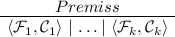
  is a (B)BI expansion rule from Figs. 3 or 4 for which a concrete instance of Premiss is fulfilled by $\langle \mathcal {F}, \mathcal {C} \rangle$, then the list $\mathcal {T}_m \oplus [ \langle \mathcal {F} \cup \mathcal {F}_1, \mathcal {C} \cup \mathcal {C}_1 \rangle ; \ldots ; \langle \mathcal {F} \cup \mathcal {F}_k, \mathcal {C} \cup \mathcal {C}_k \rangle ] \oplus \mathcal {T}_n$ is a tableau for $\langle \mathcal {F}_0, \mathcal {C}_0 \rangle$.

A (B)BI tableau for $\phi$ is a (B)BI tableau for $\langle \{ \mathbb {\mathbb {F}} \phi : c_0 \}, \emptyset \rangle$.    $\square$

Definition 2

(Closed Tableau/Proof). A CSS $\langle \mathcal {F}, \mathcal {C} \rangle$ is closed if one of the following closure conditions holds: (1) $\mathbb {\mathbb {T}} \phi : x \in \mathcal {F}$, $\mathbb {\mathbb {F}} \phi : y \in \mathcal {F}$ and $x \mathbin {\sim }y \in \mathcal {C}$; (2) $\mathbb {\mathbb {F}} \top : x \in \mathcal {F}$; (3) $\mathbb {\mathbb {T}} \bot : x \in \mathcal {F}$; (4) $\mathbb {F} \mathrm {I} : x \in \mathcal {F}$ and $Ex \in \mathcal {C}$. A CSS is open iff it is not closed. A tableau is closed iff all its branches are closed. A proof for a formula $\phi$ is a closed tableau for $\phi$.    $\square$

We note that we could simply add $\langle \mathbb {T}\lnot \rangle , \langle \mathbb {F}\lnot \rangle$, and $\langle \text {Sym} \rangle$ to the BI system and obtain one for BBI. However, this causes a significant amount of redundancy in the production of labels and constraints while requiring many more derivation steps in proofs, something that does not arise with the BBI rules given.

Fig. 5.

Separation properties.

Extension with Separation Theories. A separation property is a first-order axiom in the language of (B)BI Kripke frames. Figure 5 gives separation properties taken from across the Separation Logic literature [10, 13, 14, 24], presented as coherent formulae. A separation theory is thus a collection $\varSigma$ of axioms from Fig. 5. The syntactic form of coherent formulae enables a uniform translation of separation properties into tableaux expansion rules and closure conditions. First, each first-order atomic formula is translated into constraints: $Tr(z \in x \circ y) = R_{*}xyz$, $Tr(x \in E) = Ex$, $Tr(x \le y) = x \mathbin {\sim }y$ and $Tr(x = x') = x \mathbin {\sim }x', x' \mathbin {\sim }x$. Given with $n, m \ne 0$, we obtain the frame expansion rule

where each $\mathcal {C}_i$ is the set of constraints translated from the conjuncts of $B_i$, using fresh labels in place of the previously quantified . For example, the separation properties Cross-Split and Non-Branching are translated to the rules

where $c_i, c_j, c_k, c_l$ are fresh labels. The special case $n = 0$ gives a rule with premiss $Expr_1(x_1) , \ldots , Expr_p(x_p) \in \mathcal {F} \cup \mathcal {C}$, where each $Expr_i(x_i)$ is any expression in which $x_i$ occurs and the $x_i$ are the universally quantified variables in the original formula. The case $m=0$ gives a new closure condition consisting of the conjunction of constraints translated from the antecedent of the original formula.

Note that the property Splittability is defined by a system of coherent axioms. These axioms force the new predicate $\overline{E}$ to be interpreted as the complement of E. When translated into tableaux rules, $x \in \overline{E}$ gives a new constraint $\overline{E}x$.

Given a separation theory $\varSigma$, a (B)BI + $\varSigma$-tableau/proof is defined in the same way as Definitions 1 and 2, except that a tableau can also be expanded by translated $\varSigma$-rules, and any new closure properties obtained from $\varSigma$ can factor into the closure of a tableau and thus into proofs.

We give an example of a tableau proof in Fig. 6. The formula $(\lnot \mathrm {I} \mathbin {-*}\bot ) \rightarrow \mathrm {I}$ is valid in BBI models satisfying Total, but not in all BBI models [35], and Fig. 6—written, for clarity, using the traditional representation of tableaux and using $\otimes$ to denote closed branches—shows that the tableaux system for BBI + Total proves it. The left-hand branch is closed because both $\mathbb {F}\mathrm {I}:c_0$, $\mathbb {T}\mathrm {I}:c_0$ and $c_0 \mathbin {\sim }c_0$ occur, while the right is closed because $\mathbb {T}\bot :c_1$ occurs.

Fig. 6.

Tableau proof of $(\lnot \mathrm {I} \mathbin {-*}\bot ) \rightarrow \mathrm {I}$ in the BBI + Total system.

4 Applications to Separation Logics

A separation logic can be determined by an assertion logic to describe machine state—a theory of (B)BI generated by validity in a concrete model of (B)BI + $\varSigma$ for some separation theory $\varSigma$—and a specification logic to describe changes to machine state following program execution—typically a logic of Hoare triples $\{ \phi \} C \{ \psi \}$, where $\phi$ and $\psi$ are formulas of the assertion language and C is a program in some programming language. Soundness of the frame rule,

$$\begin{aligned} {\frac{\{ \,\phi \, \} \, C \, \{ \,\psi \, \} }{\{ \,\phi *\chi \, \} \, C \, \{ \,\psi *\chi \, \} },} \end{aligned}$$

where $\chi$ does not include any free variables modified by the program C, witnesses the coherence of these different aspects, and facilitates Separation Logic’s characteristic ‘local reasoning’, which allows conclusions about a program’s effect on the global state to be derived from reasoning on just the resource it accesses.

To demonstrate the wide applicability of our framework we now give a number of separation logics that are models of separation theories. We note that our systems can be incomplete with respect to a given concrete model, but this is as expected for any proof system: the benefit versus a standard (B)BI system—which will be incomplete with respect to the class of models of a given separation theory—is the capability to make inferences based on the additional structure the model carries. Because of space constraints this selection is demonstrative rather than exhaustive. Other examples include Petri nets [13]; step-indexed models for storable locks [11] and the Iris framework [33]; separation logics incorporating named [42] and fractional [7] permissions; and separation logics designed for message passing [49] and amortized resource analysis [3].

Heaps. Our first example is given by the standard memory models of Separation Logic [32]. A heap is a partial function $h: \mathbb {N} \rightarrow \mathbb {Z}$, representing an allocation of memory addresses to values. Given heaps $h, h'$, $h \# h'$ denotes that $dom(h) \cap dom(h') = \emptyset$; $h \cdot h'$ denotes the union of functions with disjoint domains, which is defined iff $h\#h'$. The empty heap, [], is defined nowhere.

Let H denote the set of all heaps. Then $\mathrm {Heap_{BBI}}=(H, \cdot , \{ [] \})$ is a BBI frame. Letting $h \sqsubseteq h'$ denote that $h'$ extends h, $\mathrm {Heap_{BI}}=(H, \sqsubseteq , \cdot , H)$ defines a BI frame. These frames generate the standard classical and intuitionistic models of Separation Logic. $\mathrm {Heap_{BBI}}$ satisfies Partial Determinism, Cancellativity, Single Unit, Indivisible Units, Cross-Split and Unit Self Joining; $\mathrm {Heap_{BI}}$ additionally satisfies Splittability, Upwards-Closed, Downwards-Closed, Increasing and Normal Increasing while dropping Single Unit and Unit Self Joining.

One property distinguishing the standard memory models is that $*$-elimination—$\phi * \psi \rightarrow \psi$, useful for reasoning about garbage-collected languages—is valid in the intuitionistic heap model but not the classical. Cao et al. [14] show that this corresponds to the separation property Increasing. Figure 7—written with a traditional tableau presentation—shows a single branch tableaux proof of $\phi * \psi \rightarrow \psi$ for $BI + \text {Increasing}$, closed because $\mathbb {T}\psi :c_4$, $\mathbb {F}\psi :c_1$ and $c_4 \mathbin {\sim }c_1$ occur.

Permissions. Permissions are incorporated into variants of separation logics that are designed to reason about certain kinds of concurrent algorithms and more fine-grained notions of memory disjointness: for example, disjointness modulo shared read permission. Hóu [29] reports a schema of Clouston that encompasses many such models: we recall it, with two concrete instances.

Let V be a set of values and $\star : V^2 \rightarrow V$ an associative and commutative partial function. Denote by $H_{V}$ the set of V-valued heaps $h: \mathbb {N} \rightarrow V$. Then $\mathrm {Heap}_{V} = (H_{V}, \circ _{\star }, \{ [] \})$ is a BBI frame, where $\circ _{\star }$ is defined by

$$ { h_1 \circ _{\star } h_2(n) = {\left\{ \begin{array}{ll} h_1(n) \star h_2(n) &{} \text {if } n \in dom(h_1) \cap dom(h_2) \text { and } h_1(n) \star h_2(n) \downarrow \\ h_1(n) &{} \text {if } n \in dom(h_1) \setminus dom(h_2) \\ h_2(n) &{} \text {if } n \in dom(h_2) \setminus dom(h_1) \\ \text {undefined} &{} \text {otherwise.} \end{array}\right. }} $$

Hóu defines Bornat et al.’s [6] counting permissions model with $V = \mathbb {Z}^2$ and

$$ { (x, i) \star (y, j) = {\left\{ \begin{array}{ll} (x, i+j) &{} \text {if } x=y, i< 0 \text { and } j< 0 \\ (x, i+j) &{} \text {if } x=y, i+j \ge 0 \text { and } (i< 0 \text { or } j < 0) \\ \text {undefined} &{} \text {otherwise.} \end{array}\right. }} $$

This frame satisfies Partial Determinism, Cancellativity, Indivisible Units, Single Unit, Cross-Split and Unit Self Joining.

Fig. 7.

Tableau proof of $\phi * \psi \rightarrow \psi$ in the BI + Increasing system.

Hóu defines Dockins et al.’s [24] binary tree model by considering the set T of non-empty binary trees with leaves labelled $\top$ or $\bot$ that are quotiented by the smallest congruence that identifies any subtree in which all leaves have the same label with a single leaf carrying that label. Then $V = \mathbb {Z} \times T$, and $\star$ is defined, where $\vee$ ($\wedge$) denotes pointwise disjunction (conjunction) of equivalent trees, by

$$ { (x, [t]) \star (y, [t']) = {\left\{ \begin{array}{ll} (x, [t \vee t']) &{} \text { if } x=y \text { and } [t \wedge t'] = [ \bot ] \\ \text {undefined} &{} \text { otherwise.} \end{array}\right. }} $$

This frame satisfies Partial Determinism, Cancellativity, Single Unit, Indivisible Units, Disjointness, Splittability, Cross-Split and Unit Self Joining.

Crash Hoare Logic. Chen et al. [16] use a separation logic to verify that the FSCQ file system meets its specification and secures its data under any sequence of crashes. Cao et. al. [14] give the underlying model as the following BI frame. Let $V^{+}$ be the set of non-empty lists over a set V and $\epsilon$ the empty list. Buffer heaps are defined to be heaps $h: \mathbb {N} \rightarrow V^{+}$. Let $H_{\mathrm {buff}}$ be the set of all buffer heaps. Then $Heap_{\mathrm {buff}} = (H_{\mathrm {buff}}, \le , \cdot , \{ [] \} )$ is a BI frame, where $\cdot$ is the usual heap composition, and $h_1 \le h_2$ iff $dom(h_1) = dom(h_2)$ and $\forall x \in \mathbb {N}$, $\exists l \in V^{+} \cup \{ \epsilon \}$ such that $h_1(x) = l \oplus h_2(x)$. This frame satisfies Partial Determinism, Cancellativity, Single Unit, Indivisible Units, Cross-Split, Upwards-Closed, Downwards-Closed, Always-Joins, Non-Branching, Unit Self Joining, and Normal Increasing.

Typed Heaps. Cao et al. [14] give an example derived from the handling of multibyte locks in Appel’s [2] Verified System Toolchain separation logic for CompCert C. Let a typed heap be a partial map $h: \mathbb {N} \rightarrow \{ \mathrm {char, short}_1, \mathrm {short}_2\}$ such that $h(n) = \mathrm {short}_1$ implies $h(n+1) = \mathrm {short}_2$. Let $H_{\mathrm {typ}}$ denote the set of all typed heaps. Then $\mathrm {Heap}_{\mathrm {Typ}} = (H_{\mathrm {typ}}, \le , \circ , H_{\mathrm {typ}})$ is a BI frame, where $h_1 \le h_2$ iff, for all $n \in dom(h_1)$ either $n \in dom(h_2)$ and $h_1(n) = h_2(n)$ or $h_1(n) = \mathrm {char}$, and $h \in h_1 \circ h_2$ iff $h_1 \cdot h_2 \le h$. This frame satisfies Indivisible Units, Disjointness, Splittability, Cross-Split, Upwards-Closed, Downwards-Closed, Non-Branching, Increasing, and Normal Increasing.

5 Metatheory

Tableaux Systems as Coherent Theories. Just as coherent formulae yield tableaux rules, tableaux rules yield coherent formulae, allowing a complete specification of our calculi as coherent theories. Our framework determines a first-order signature: for each formula $\phi$ of (B)BI, we have unary relation symbols $\mathbb {T}\phi$ and $\mathbb {F}\phi$, together with the unary relation symbol E, the binary relation symbol $\mathbin {\sim }$ and the ternary relation symbol $R_{*}$.

Given a rule premiss ‘$\mathbb {S}\phi :x \in \mathcal {F}$ and $A_1x^1_1\ldots x^1_{k_1}, \ldots , A_m x^m_1\ldots x^m_{k_m} \in \mathcal {C}$’ we obtain the coherent antecedent . For the $j-th$ conclusion $\langle \mathcal {F}_j, \mathcal {C}_j \rangle$ of the rule we obtain , where $C_j$ is the conjunction of atomic formulae translated from the constraints in $\mathcal {F}_j \cup \mathcal {C}_j$, with any fresh labels that occurred substituted with . The translated rule is thus . For example, the instance of the BI rule $\langle \mathbb {F} \mathbin {-*}\rangle$ for $\phi \mathbin {-*}\psi$ becomes $\mathbb {F}\phi \mathbin {-*}\psi (x) \rightarrow \exists y_1, y_2, y_3(\mathbb {T}\phi (y_2) \wedge \mathbb {F}\psi (y_3) \wedge x \mathbin {\sim }y_1 \wedge R_{*}y_1y_2y_3)$.

There are some special cases to pay attention to. For tableaux rules with premiss $\mathrm {Expr}(x) \in \mathcal {F} \cup \mathcal {C}$ the antecedent of the translated coherent formula is $\top$. This is not the case for rules with premiss $\mathrm {Expr}(x) \in \mathcal {C}$: these must be translated into a separate rule for each of the finitely many ways x can occur in each constraint. Finally, each closure condition ‘$\mathbb {S}_1\phi _1:x_1 , \ldots , \mathbb {S}_n\phi _n:x_n$, $A_1y^1_1\ldots y^1_{k_1}, \ldots$, and $A_m y^m_1\ldots y^m_{k_m}$’ gives $\bigwedge _{i} \mathbb {S}_i\phi _i(x_i) \wedge \bigwedge _{i} A_i y^i_1 \ldots y^i_{k_i} \rightarrow \bot .$

Given a (B)BI formula $\phi$, the finite coherent theory $\varPhi _{\phi }^{(B)BI + \varSigma }$ is given by the translated $(B)BI + \varSigma$-frame expansion rules, the translated closure conditions and the instances of translated logical expansion rules for subformulae of $\phi$. We note that we could specify the whole tableaux system for (B)BI + $\varSigma$ as an infinite coherent theory (similar to the axiomatization of a Hintikka set in standard tableaux completeness proofs), but finiteness is required for our argument.

Soundness and Completeness. We now prove soundness and completeness of the tableaux method via an analogous result for the Tarskian semantics of coherent logic. First, we show that the existence of a Kripke $(B)BI + \varSigma$-model with a state that doesn’t satisfy $\phi$ is equivalent to the existence of a Tarskian model of $\varPhi _{\phi }^{(B)BI + \varSigma } \cup \{ \exists x. \mathbb {F}\phi (x) \}$.

Definition 3

(Induced Kripke Model of $\mathcal {M}$). Given a Tarskian model $\mathcal {M}$ of $\varPhi _{\phi }^{(B)BI + \varSigma }$, define $[a] = \{ b \mid a \mathbin {\sim }^{\mathcal {I}} b, b \mathbin {\sim }^{\mathcal {I}} a \}$ and $X_{\mathcal {M}} = \{ [ a ] \mid a \in X \}$. Then $[a] \le _{\mathcal {M}} [b]$ iff $a \mathbin {\sim }^{\mathcal {I}} b$, $[c] \in [a] \circ _{\mathcal {M}}[b]$ iff $R^{\mathcal {I}}_{*}abc$, and $E_{\mathcal {M}} = \{ [a] \mid E^{\mathcal {I}}a \}$. $\mathcal {V}_{\mathcal {M}}(\mathrm{p}) = \{ [a] \mid \exists b(b \mathbin {\sim }^{\mathcal {I}} a \text { and } \mathbb {T}\mathrm{p}^{\mathcal {I}}(b)) \}$.

• 1. If $\mathcal {M}$ is a model of $\varPhi _{\phi }^{BI + \varSigma }$, the induced Kripke frame is given by $\mathcal {X}_{\mathcal {M}} = (X_{\mathcal {M}}, \le _{\mathcal {M}}, \circ _{\mathcal {M}}, E_{\mathcal {M}})$; the induced Kripke model is given by $(\mathcal {X}_{\mathcal {M}}, \mathcal {V}_{\mathcal {M}})$.

• 2. If $\mathcal {M}$ is a model of $\varPhi _{\phi }^{BBI + \varSigma }$, the induced Kripke frame is given by $\mathcal {X}_{\mathcal {M}} = (X_{\mathcal {M}}, \circ _{\mathcal {M}}, E_{\mathcal {M}})$; the induced Kripke model is given by $(\mathcal {X}_{\mathcal {M}}, \mathcal {V}_{\mathcal {M}})$.

The induced Kripke frame is a well-defined structure because of the frame tableaux rules, with $[-]$ forming equivalence classes and $\le _{\mathcal {M}}$, $\circ _{\mathcal {M}}$, and $E_{\mathcal {M}}$ independent from the choice of representatives due to $\langle \text {Cong} \rangle$. The $(B)BI + \varSigma$-frame properties for the induced frame follow from their correspondent rules in the tableaux and the valuation $\mathcal {V}_{\mathcal {M}}$ is independent of choice of representative and persistent for induced Kripke $BI+\varSigma$-models.

Lemma 1

Given a Tarskian model $\mathcal {M}$ of $\varPhi _{\phi }^{(B)BI + \varSigma }$, the induced Kripke model $\mathcal {X}_{\mathcal {M}}$ is a Kripke $(B)BI + \varSigma$-model.    $\square$

The significance of this model is that satisfiability of subformulae $\psi$ of $\phi$ is determined by the interpretation of the relation symbols $\mathbb {S}\psi$ in the original Tarskian model. A simple proof by induction yields the next lemma.

Lemma 2

Let $\mathcal {M}$ be a Tarskian model of the coherent theory $\varPhi ^{(B)BI + \varSigma }_{\phi }$, $\psi$ a subformula of $\phi$ and $a \in X$. 1. If $\mathbb {T}\psi ^{\mathcal {I}}(a)$ holds in $\mathcal {M}$, then $[ a ] \vDash _{\mathcal {V}_{\mathcal {M}}} \psi$; 2. If $\mathbb {F}\psi ^{\mathcal {I}}(a)$ holds in $\mathcal {M}$, then $[a] \not \vDash _{\mathcal {V}_{\mathcal {M}}} \psi$.    $\square$

We can also induce Tarskian models from Kripke models. Let $(\mathcal {X}, \mathcal {V})$ be a Kripke $(B)BI + \varSigma$-model. We define the induced Tarskian model by taking X to be the carrier, and defining the interpretation $\mathcal {I}$ by $\mathbin {\sim }^{\mathcal {I}} = {\ }\le$, $R_{*}^{\mathcal {I}} = \{ (a, b, c) \mid c \in a \circ b \}$, $E^{\mathcal {I}} = E$, $\mathbb {T}\psi ^{\mathcal {I}} = \{ x \mid x \vDash _{\mathcal {V}} \psi \}$ and $\mathbb {F}\psi ^{\mathcal {I}} = \{ x \mid x \not \vDash _{\mathcal {V}} \psi \}$.

Lemma 3

Every Kripke $(B)BI \!+\! \varSigma$-model $(\mathcal {X}, \mathcal {V})$ with a state x (not) satisfying $\phi$ induces a model of $\varPhi _{\phi }^{(B)BI + \varSigma } \cup \{ \exists x. \mathbb {T}\phi (x) \}$ ($\varPhi _{\phi }^{(B)BI + \varSigma } \cup \{ \exists x. \mathbb {F}\phi (x) \}$).    $\square$

We now connect the existence of a closed tableaux to Bezem and Coquand’s [4] breadth-first forward reasoning proof system for coherent logic. In their system, judgments of the form $X \Vdash ^{\varPhi } D$ are derived, where X is a set of atomic first-order sentences, $\varPhi$ a finite coherent theory and D a closed coherent disjunction; a first-order sentence with the same syntactic shape as the consequent of a coherent formula. The derivation of the judgment $X \Vdash ^{\varPhi } D$ is defined inductively:

• 1. (Base): $X \Vdash ^{\varPhi } D$ holds if for one of the disjuncts of D, there are constants such that all conjuncts of occur in X;

• 2. (Inductive Step): Consider all closed instances $C_i \rightarrow D_i$ of $\varPhi$-axioms such that the conjuncts of $C_i$ occur in X but the conjuncts of no disjunct $C_{i, j}$ of $D_i$ do. There exist finitely many, with their consequents thus enumerated $D_0, \ldots , D_n$. Let denote the j-th of the $m_i$ disjuncts of $D_i$, and denote by $\overline{C_{i,j}}$ the substitution of with fresh constants. Infer $X \Vdash ^{\varPhi } D$ from $\forall j_0 \in \{1, \ldots , m_0 \}, \ldots ,\forall j_n \in \{1, \ldots , m_n \} (X, \overline{C_{0, j_0}}, \ldots , \overline{C_{n, j_n}} \Vdash ^{\varPhi } D).$ Importantly, if a $D_i$ is $\bot$, then $m_i = 0$, and $X \Vdash ^{\varPhi } D$ is trivially inferred.

A derivation can be seen as a kind of tableau, branching at each stage by adding every possible consequence of $\varPhi$ obtainable from the atomic first-order sentences at the current node. A semi-decidable procedure is given to systematically search for a derivation of $X \Vdash ^{\varPhi } D$. First check the base case. If it doesn’t hold, apply the inductive step to any $\varPhi$-axioms fireable from X. If there are none, X forms an Herbrand countermodel of $\varPhi$ against D. If the inductive step can be applied, apply the search procedure recursively to all premisses. Bezem and Coquand show that successful termination corresponds to Tarskian truth.

Theorem 1

([4]). $X \Vdash ^{\varPhi } D$ is derivable iff the search procedure successfully terminates for $X \Vdash ^{\varPhi } D$ iff D is true in all Tarskian models of $X \cup \varPhi$.   $\square$

It is straightforward that the search procedure for $\{ \mathbb {F}\phi (a) \} \Vdash ^{\varPhi ^{(B)BI + \varSigma }_{\phi }} \bot$ corresponds precisely to an exhaustive search for a closed tableau for $\phi$.

Lemma 4

There exists a closed $(B)BI + \varSigma$-tableaux for $\phi$ iff the search procedure for $\{ \mathbb {F}\phi (a) \} \Vdash ^{\varPhi ^{(B)BI + \varSigma }_{\phi }} \bot$ successfully terminates.    $\square$

Hence if a closed $(B)BI + \varSigma$-tableaux does not exist for $\phi$, there exists a Tarskian model $\mathcal {M}$ of $\varPhi ^{(B)BI+\varSigma }_{\phi } \cup \{ \exists x. \mathbb {F}\phi (x) \}$. By Lemma 2, the induced Kripke model $\mathcal {X}_{\mathcal {M}}$ has a state [a] such that $[a] \not \vDash _{\mathcal {V}_{\mathcal {M}}} \phi$, establishing that $\phi$ fails to be valid for Kripke $(B)BI + \varSigma$-models. Conversely, if a closed tableaux does exist, then there is no Tarskian model of $\mathcal {M}$ of $\varPhi ^{(B)BI+\varSigma }_{\phi } \cup \{ \exists x. \mathbb {F}\phi (x) \}$. By Lemma 3, $\phi$ is valid in Kripke $(B)BI + \varSigma$-models, as otherwise any countermodel would generate a Tarskian model $\mathcal {M}$ of $\varPhi ^{(B)BI+\varSigma }_{\phi } \cup \{ \exists x. \mathbb {F}\phi (x) \}$, a contradiction.

Theorem 2

(Soundness and Completeness for $(B)BI \!+\! \varSigma$-Tableaux). $\phi$ is valid in Kripke $(B)BI + \varSigma$-models iff $\phi$ is provable in the $(B)BI + \varSigma$-tableaux system.    $\square$

6 Conclusions and Further Work

We have given a framework of tableaux systems that exhaustively captures the breadth of separation theories in the literature. Our framework is proven sound and complete parametrically by a novel representation of tableaux systems as coherent theories that allows us to apply existing theory from coherent logic. This resolves the expressivity gap between the logics of bunched implications and the separation logics defined upon them, and provides proof theory for the assertion languages of a wide array of program logics.

The completeness of tableaux systems is usually proved by defining a notion of a Hintikka set: a saturated set of (labelled) formulae (and possibly constraints) that specifies a term model of the logic. The existence of a Hintikka set is then shown to follow from non-existence of a tableau proof. Our method is a generalization of this idea, implemented parametrically by choice of tableaux system. While we have focused on Separation Logic, this technique is adaptable to virtually any logic interpreted on relational structures, including the breadth of bunched and modal logics. This suggests the significance of the coherent logic fragment extends beyond the generation of proof rules for frame conditions.

The implementation of our systems is of principal importance for future work. Our tableaux representation suggests existing coherent logic provers (see [43] for a survey) may already be suitable, though tactics designed specifically for tableaux coherent theories may have to be developed to make this efficient. A closely related goal is the development of parametric Separation Logic implementations that utilize our systems as assertion language provers. Finally, our results suggest interesting theoretical work. Coherent logic has close connections to topos theory, and Caramello [15] has developed techniques to transfer results between mathematical fields via bridges between the classifying topoi of coherent theories. We wish to investigate if any results of logical interest can be found in this way by utilizing the representation of tableaux as coherent theories.

References

Anderson, G., Pym, D.: A calculus and logic of bunched resources and processes. Theoret. Comput. Sci. 614, 63–96 (2016)
Appel, A.W.: Program Logics for Certified Compilers. CUP (2014)
Atkey, R.: Amortised resource analysis with separation logic. Log. Methods Comput. Sci. 2(17), 1–33 (2011)
Bezem, M., Coquand, T.: Automating coherent logic. In: Sutcliffe, G., Voronkov, A. (eds.) LPAR 2005. LNCS (LNAI), vol. 3835, pp. 246–260. Springer, Heidelberg (2005). https://doi.org/10.1007/11591191_18
Berdine, J., Calcagno, C., O’Hearn, P.W.: Smallfoot: modular automatic assertion checking with separation logic. In: de Boer, F.S., Bonsangue, M.M., Graf, S., de Roever, W.-P. (eds.) FMCO 2005. LNCS, vol. 4111, pp. 115–137. Springer, Heidelberg (2006). https://doi.org/10.1007/11804192_6
Bornat, R., Calcagno, C., O’Hearn, P., Parkinson, M.: Permission accounting in separation logic. In: Proceedings of POPL 2005, pp. 259–270. ACM (2005)
Boyland, J.: Checking interference with fractional permissions. In: Cousot, R. (ed.) SAS 2003. LNCS, vol. 2694, pp. 55–72. Springer, Heidelberg (2003). https://doi.org/10.1007/3-540-44898-5_4
Braüner, T.: Hybrid Logic and Its Proof-Theory. Applied Logic Series, vol. 37. Springer, Dordrecht (2011)
Brotherston, J.: Bunched logics displayed. Stud. Logica. 100(6), 1223–1254 (2012)
Brotherston, J., Villard, J.: Parametric completeness for separation theories. In: Proceedings of POPL 2014, pp. 453–464. ACM (2014)
Buisse, A., Birkedal, L., Støvring, K.: A step-indexed Kripke model of separation logic for storable locks. In: Proceedings of MFPS XXVII, ENTCS, vol. 276, pp. 121–143 (2011)
Calcagno, C., Distefano, D., O’Hearn, P., Yang, H.: Compositional shape analysis by means of bi-abduction. J. ACM 58(6), 26 (2011). https://doi.org/10.1145/2049697.2049700
Calcagno, C., O’Hearn, P., Yang, H.: Local action and abstract separation logic. In: Proceedings of LICS 2007, pp. 366–378. IEEE (2007)
Cao, Q., Cuellar, S., Appel, A.W.: Bringing order to the separation logic jungle. In: Chang, B.-Y.E. (ed.) APLAS 2017. LNCS, vol. 10695, pp. 190–211. Springer, Cham (2017). https://doi.org/10.1007/978-3-319-71237-6_10
Caramello, O.: Theories, Sites, Toposes: Relating and Studying Mathematical Theories Through Topos-Theoretic ‘Bridges’. OUP, Oxford (2017)
Chen, H., Ziegler, D., Chajed, T., Chlipala, A., Kaashoek, M.F., Zeldovich, N.: Using crash hoare logic for certifying the FSCQ file system. In: Proceedings of SOSP 2015, pp. 18–37. ACM (2015)
Collinson, M., McDonald, K., Pym, D.: A substructural logic for layered graphs. J. Log. Comput. 24(4), 953–988 (2014)
Collinson, M., McDonald, K., Pym, D.: Layered graph logic as an assertion language for access control policy models. J. Log. Comput. 27(1), 41–80 (2017)
Collinson, M., Pym, D.: Algebra and logic for resource-based systems modelling. Math. Struct. Comput. Sci. 19, 959–1027 (2009)
Courtault, J.-R., Galmiche, D., Pym, D.: A logic of separating modalities. Theoret. Comput. Sci. 637, 30–58 (2016)
Dinsdale-Young, T., Birkedal, L., Gardner, P., Parkinson, M., Yang, H.: Views: compositional reasoning for concurrent programs. In: Proceedings of POPL 2013, pp. 287–300 (2013)
Docherty, S., Pym, D.: Intuitionistic layered graph logic. In: Olivetti, N., Tiwari, A. (eds.) IJCAR 2016. LNCS (LNAI), vol. 9706, pp. 469–486. Springer, Cham (2016). https://doi.org/10.1007/978-3-319-40229-1_32
Docherty, S., Pym, D.: Stone-Type Dualities for Separation Logics (Submitted)
Dockins, R., Hobor, A., Appel, A.W.: A fresh look at separation algebras and share accounting. In: Hu, Z. (ed.) APLAS 2009. LNCS, vol. 5904, pp. 161–177. Springer, Heidelberg (2009). https://doi.org/10.1007/978-3-642-10672-9_13
Dyckhoff, R., Negri, S.: Geometrisation of first-order logic. Bull. Symb. Log. 21(2), 123–163 (2015)
Galmiche, D., Kimmel, P., Pym, D.: A substructural epistemic resource logic. In: Ghosh, S., Prasad, S. (eds.) ICLA 2017. LNCS, vol. 10119, pp. 106–122. Springer, Heidelberg (2017). https://doi.org/10.1007/978-3-662-54069-5_9
Galmiche, D., Méry, D.: Tableaux and resource graphs for separation logic. J. Log. Comput. 20(1), 189–231 (2007)
Galmiche, D., Méry, D., Pym, D.: The semantics of BI and resource tableaux. Math. Struct. Comput. Sci. 15, 1033–1088 (2005)
Hóu, Z.: Labelled sequent calculi and automated reasoning for assertions in separation logic. Ph.D. thesis, The Australian National University (2015)
Hóu, Z., Goré, R., Tiu, A.: Automated theorem proving for assertions in separation logic with all connectives. In: Felty, A.P., Middeldorp, A. (eds.) CADE 2015. LNCS (LNAI), vol. 9195, pp. 501–516. Springer, Cham (2015). https://doi.org/10.1007/978-3-319-21401-6_34
Hóu, Z., Clouston, R., Tiu, A., Goré, R.: Proof search for propositional abstract separation logics via labelled sequents. In: Proceedings of POPL 2014, pp. 465–476. ACM (2014)
Ishtiaq, S., O’Hearn, P.: BI as an assertion language for mutable data structures. In: Proceedings of POPL 2001, 14–26. ACM (2001)
Jung, R., Krebbers, R., Jourdan, J.-H., Bizjak, A., Birkedal, L., Dreyer, D.: Iris from the ground up: a modular foundation for higher-order concurrent separation logic (2017). Under consideration for publication in Journal of Functional Programming
Larchey-Wendling, D.: The formal strong completeness of partial monoidal Boolean BI. J. Log. Comput. 26(2), 605–640 (2016)
Larchey-Wendling, D., Galmiche, D.: The undecidability of Boolean BI through phase semantics. In: Proceedings of LICS 2010, pp. 140–149. IEEE Computer Society Press (2010)
Larchey-Wendling, D., Galmiche, D.: Looking at separation algebras with Boolean BI-eyes. In: Diaz, J., Lanese, I., Sangiorgi, D. (eds.) TCS 2014. LNCS, vol. 8705, pp. 326–340. Springer, Heidelberg (2014). https://doi.org/10.1007/978-3-662-44602-7_25
Nakano, H.: A modality for recursion. In: Proceedings of LICS 2000, pp. 255–266. IEEE (2000)
Negri, S.: Proof analysis beyond geometric theories: from rule systems to systems of rules. J. Log. Comput. 26(2), 513–537 (2016)
O’Hearn, P.: A Primer on Separation Logic. Software Safety and Security. NATO Science for Peace and Security Series, vol. 33, pp. 286–318 (2012)
O’Hearn, P., Pym, D.: The logic of bunched implications. Bull. Symb. Log. 5(2), 215–244 (1999)
Park, J., Seo, J., Park, S.: A theorem prover for BBI. In: Proceedings of POPL 2013, pp. 219–232. ACM (2013)
Parkinson, M.: Local reasoning for Java. Ph.D. thesis, University of Cambridge (2005)
Polonsky, A.: Proofs, Types and Lambda Calculus. Ph.D. thesis, University of Bergen (2012)
Reynolds, J.: Separation logic: a logic for shared mutable data structures. In: Proceedings of LICS 2002, pp. 55–74. IEEE Computer Society Press (2002)
Schmidt, R.A., Tishkovsky, D.: Automated synthesis of tableau calculi. In: Giese, M., Waaler, A. (eds.) TABLEAUX 2009. LNCS (LNAI), vol. 5607, pp. 310–324. Springer, Heidelberg (2009). https://doi.org/10.1007/978-3-642-02716-1_23
Simpson, A.: The proof theory and semantics of intuitionistic modal logic. Ph.D. thesis, University of Edinburgh (1994)
Skolem, T.: Logisch-kombinatorische Untersuchungen über die Erfüllbarkeit und Beweisbarkeit mathematischen Sätze nebst einem Theoreme über dichte Mengen, Skrifter I, vol. 4, pp. 1–36. Det Norske Videnskaps-Akademi, (1920)
Terese: Term Rewriting Systems. Cambridge University Press (2003)
Villard, J., Lozes, É., Calcagno, C.: Proving copyless message passing. In: Hu, Z. (ed.) APLAS 2009. LNCS, vol. 5904, pp. 194–209. Springer, Heidelberg (2009). https://doi.org/10.1007/978-3-642-10672-9_15
Yang, H., O’Hearn, P.: A semantic basis for local reasoning. In: Nielsen, M., Engberg, U. (eds.) FoSSaCS 2002. LNCS, vol. 2303, pp. 402–416. Springer, Heidelberg (2002). https://doi.org/10.1007/3-540-45931-6_28
Author information
Authors and Affiliations
Corresponding author
Editor information
Editors and Affiliations
Rights and permissions
Open Access This chapter is licensed under the terms of the Creative Commons Attribution 4.0 International License (http://creativecommons.org/licenses/by/4.0/), which permits use, sharing, adaptation, distribution and reproduction in any medium or format, as long as you give appropriate credit to the original author(s) and the source, provide a link to the Creative Commons license and indicate if changes were made. The images or other third party material in this book are included in the book's Creative Commons license, unless indicated otherwise in a credit line to the material. If material is not included in the book's Creative Commons license and your intended use is not permitted by statutory regulation or exceeds the permitted use, you will need to obtain permission directly from the copyright holder.
Copyright information
© 2018 The Author(s)
About this paper
Cite this paper
Docherty, S., Pym, D. (2018). Modular Tableaux Calculi for Separation Theories. In: Baier, C., Dal Lago, U. (eds) Foundations of Software Science and Computation Structures. FoSSaCS 2018. Lecture Notes in Computer Science(), vol 10803. Springer, Cham. https://doi.org/10.1007/978-3-319-89366-2_24
Download citation
DOI: https://doi.org/10.1007/978-3-319-89366-2_24
Published:
Publisher Name: Springer, Cham
Print ISBN: 978-3-319-89365-5
Online ISBN: 978-3-319-89366-2
eBook Packages: Computer ScienceComputer Science (R0)