Iterative Generation of Diverse Models for Testing Specifications of DSL Tools

Abstract

The validation of modeling tools of custom domain-specific languages (DSLs) frequently relies upon an automatically generated set of models as a test suite. While many software testing approaches recommend that this test suite should be diverse, model diversity has not been studied systematically for graph models. In the paper, we propose diversity metrics for models by exploiting neighborhood shapes as abstraction. Furthermore, we propose an iterative model generation technique to synthesize a diverse set of models where each model is taken from a different equivalence class as defined by neighborhood shapes. We evaluate our diversity metrics in the context of mutation testing for an industrial DSL and compare our model generation technique with the popular model generator Alloy.

1 Introduction

Motivation. Domain-Specific Language (DSL) based modeling tools are gaining an increasing role in the software development processes. Advanced DSL frameworks such as Xtext, or Sirius built on top of model management frameworks such as Eclipse Modeling Framework (EMF) [37] significantly improve productivity of domain experts by automating the production of rich editor features.

Modelling environments may provide validation for the system under design from an early stage of development with efficient tool support for checking well-formedness (WF) constraints and design rules over large model instances of the DSL using tools like Eclipse OCL [24] or graph queries [41]. Model generation techniques [16, 19, 35, 39] are able to automatically provide a range of solution candidates for allocation problems [19], model refactoring or context generation [21]. Finally, models can be processed by query-based transformations or code generators to automatically synthesize source code or other artifacts.

The design of complex DSLs tools is a challenging task. As the complexity of DSL tools increases, special attention is needed to validate the modeling tools themselves (e.g. for tool qualification purposes) to ensure that WF constraints and the preconditions of model transformation and code generation functionality [4, 32, 35] are correctly implemented in the tool.

Problem Statement. There are many approaches aiming to address the testing of DSL tools (or transformations) [1, 6, 42] which necessitate the automated synthesis of graph models to serve as test inputs. Many best practices of testing (such as equivalence partitioning [26], mutation testing [18]) recommends the synthesis of diverse graph models where any pairs of models are structurally different from each other to achieve high coverage or a diverse solution space.

While software diversity is widely studied [5], existing diversity metrics for graph models are much less elaborate [43]. Model comparison techniques [38] frequently rely upon the existence of node identifiers, which can easily lead to many isomorphic models. Moreover, checking graph isomorphism is computationally very costly. Therefore practical solutions tend to use approximate techniques to achieve certain diversity by random sampling [17], incremental generation [19, 35], or using symmetry breaking predicates [39]. Unlike equivalence partitions which capture diversity of inputs in a customizable way for testing traditional software, a similar diversity concept is still missing for graph models.

Contribution. In this paper, we propose diversity metrics to characterize a single model and a set of models. For that purpose, we innovatively reuse neighborhood graph shapes [28], which provide a fine-grained typing for each object based on the structure (e.g. incoming and outgoing edges) of its neighborhood. Moreover, we propose an iterative model generation technique to automatically synthesize a diverse set of models for a DSL where each model is taken from a different equivalence class wrt. graph shapes as an equivalence relation.

We evaluate our diversity metrics and model generator in the context of mutation-based testing [22] of WF constraints in an industrial DSL tool. We evaluate and compare the mutation score and our diversity metrics of test suites obtained by (1) an Alloy based model generator (using symmetry breaking predicates to ensure diversity), (2) an iterative graph solver based generator using neighborhood shapes, and (3) from real models created by humans. Our finding is that a diverse set of models derived along different neighborhood shapes has better mutation score. Furthermore, based on a test suite with 4850 models, we found that high correlation between mutation score and our diversity metrics, which indicates that our metrics may be good predictors in practice for testing.

Added Value. Up to our best knowledge, our paper is one of the first studies on (software) model diversity. From a testing perspective, our diversity metrics provide a stronger characterization of a test suite of models than traditional metamodel coverage which is used in many research papers. Furthermore, model generators using neighborhood graph shapes (that keep models only if they are surely non-isomorphic) provide increased diversity compared to symmetry breaking predicates (which exclude models if they are surely isomorphic).

2 Preliminaries

Core modeling concepts and testing challenges of DSL tools will be illustrated in the context of Yakindu Statecharts [46], which is an industrial DSL for developing reactive, event-driven systems, and supports validation and code generation.

2.1 Metamodels and Instance Models

Metamodels define the main concepts, relations and attributes of a domain to specify the basic graph structure of models. A simplified metamodel for Yakindu state machines is illustrated in Fig. 1 using the popular Eclipse Modeling Framework (EMF) [37] is used for domain modeling. A state machine consists of , which in turn contain states (called ) and . An abstract state is further refined into (like or ) and (like or ).

Fig. 1.

Metamodel extract from Yakindu state machines

Formally [32, 34], a metamodel defines a vocabulary of type and relation symbols where a unary predicate symbol is defined for each EClass, and a binary predicate symbol is derived for each EReference. For space considerations, we omit the precise handling of attributes.

An instance model can be represented as a logic structure $M = \langle { Obj _{M}}, {\mathcal {I}_{M}} \rangle$ where $Obj _{M}$ is the finite set of objects (the size of the model is $| M | = | Obj _{M} |$), and $\mathcal {I}_{M}$ provides interpretation for all predicate symbols in $\varSigma$ as follows:

• the interpretation of a unary predicate symbol is defined in accordance with the types of the EMF model: 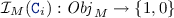An object $o \in Obj _{M}$ is an instance of a class in a model M if .

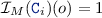• the interpretation of a binary predicate symbol is defined in accordance withe the links in the EMF model: There is a reference between $o_1, o_2 \in Obj _{M}$ in model M if

A metamodel also specifies extra structural constraints (type hierarchy, multiplicities, etc.) that need to be satisfied in each valid instance model [32].

Example 1

Figure 2 shows graph representations of three (partial) instance models. For the sake of clarity, and inverse relations and are excluded from the diagram. In $M_1$ there are two (s1 and s2), which are connected to a loop via t2 and t3. The initial state is marked by a t1 from an entry e1 to state s1. $M_2$ describes a similar statechart with three states in loop (s3, s4 and s5 connected via t5, t6 and t7). Finally, in $M_3$ there are two main differences: there is an incoming t11 to an state (e3), and there is a s7 that does not have outgoing transition. While all these M1 and M2 are non-isomorphic, later we illustrate why they are not diverse.

Fig. 2.

Example instance models (as directed graphs)

Fig. 3.

Inductive semantics of graph predicates

2.2 Well-Formedness Constraints as Logic Formulae

In many industrial modeling tools, WF constraints are captured either by OCL constraints [24] or graph patterns (GP) [41] where the latter captures structural conditions over an instance model as paths in a graph. To have a unified and precise handling of evaluating WF constraints, we use a tool-independent logic representation (which was influenced by [29, 32, 34]) that covers the key features of concrete graph pattern languages and a first-order fragment of OCL.

Syntax. A graph predicate is a first order logic predicate $\varphi (v_1, \ldots v_n)$ over (object) variables which can be inductively constructed by using class and relation predicates and , equality check $=$, standard first order logic connectives $\lnot$, $\vee$, $\wedge$, and quantifiers $\exists$ and $\forall$.

Semantics. A graph predicate $\varphi (v_1,\ldots ,v_n)$ can be evaluated on model M along a variable binding $Z:\{v_1,\ldots ,v_n\} \rightarrow Obj _{M}$ from variables to objects in M. The truth value of $\varphi$ can be evaluated over model M along the mapping Z (denoted by ${[\![ \varphi (v_1,\ldots ,v_n) ]\!]}^{M}_Z$) in accordance with the semantic rules defined in Fig. 3.

If there is a variable binding Z where the predicate $\varphi$ is evaluated to $1$ over M is often called a ${pattern\, match}$, formally ${[\![ \varphi ]\!]}^{M}_{Z} = 1$. Otherwise, if there are no bindings Z to satisfy a predicate, i.e. ${[\![ \varphi ]\!]}^{M}_{Z} = 0$ for all Z, then the predicate $\varphi$ is evaluated to $0$ over M. Graph query engines like [41] can retrieve (one or all) matches of a graph predicate over a model. When using graph patterns for validating WF constraints, a match of a pattern usually denotes a violation, thus the corresponding graph formula needs to capture the erroneous case.

2.3 Motivation: Testing of DSL Tools

A code generator would normally assume that the input models are well-formed, i.e. all WF constraints are validated prior to calling the code generator. However, there is no guarantee that the WF constraints actually checked by the DSL tool are exactly the same as the ones required by the code generator. For instance, if the validation forgets to check a subclause of a WF constraint, then runtime errors may occur during code generation. Moreover, the precondition of the transformation rule may also contain errors. For that purpose, WF constraints and model transformations of DSL tools can be systematically tested.Alternatively, model validation can be interpreted as a special case of model transformation, where precondition of the transformation rules are fault patterns, and the actions place error markers on the model [41].

A popular approach for testing DSL tools is mutation testing [22, 36] which aims to reveal missing or extra predicates by (1) deriving a set of mutants (e.g. WF constraints in our case) by applying a set of mutation operators. Then (2) the test suite is executed for both the original and the mutant programs, and (3) their output are compared. (4) A mutant is killed by a test if different output is produced for the two cases (i.e. different match set). (5) The mutation score of a test suite is calculated as the ratio of mutants killed by some tests wrt. the total number of mutants. A test suite with better mutation score is preferred [18].

Fault Model and Detection. As a fault model, we consider omission faults in WF constraints of DSL tools where some subconstraints are not actually checked. In our fault model, a WF constraint is given in a conjunctive normal form $\varphi _e = \varphi _1 \wedge \dots \wedge \varphi _k$, all unbound variables are quantified existentially ($\exists$), and may refer to other predicates specified in the same form. Note that this format is equivalent to first order logic, and does not reduce the range of supported graph predicates. We assume that in a faulty predicate (a mutant) the developer may forget to check one of the predicates $\varphi _i$ (Constraint Omission, CO), i.e. $\varphi _e = [\varphi _1\wedge \ldots \wedge \varphi _i\wedge \ldots \wedge \varphi _k]$ is rewritten to $\varphi _f = [\varphi _1 \wedge \dots \wedge \varphi _{i-1} \wedge \varphi _{i+1} \wedge \dots \wedge \varphi _k]$, or may forgot a negation (Negation Omission), i.e. $\varphi _e = [\varphi _1\wedge \ldots \wedge (\lnot \varphi _i)\wedge \ldots \wedge \varphi _k]$ is rewritten to $\varphi _f = [\varphi _1\wedge \ldots \wedge \varphi _i\wedge \ldots \wedge \varphi _k]$. Given an instance model M, we assume that both ${[\![ \varphi _e ]\!]}^{M}_{}$ and the faulty ${[\![ \varphi _f ]\!]}^{M}_{}$ can be evaluated separately by the DSL tool. Now a test model M detects a fault if there is a variable binding Z, where the two evaluations differ, i.e. ${[\![ \varphi _e ]\!]}^{M}_{Z} \ne {[\![ \varphi _f ]\!]}^{M}_{Z}$.

Example 2

Two WF constraints checked by the Yakindu environment can be captured by graph predicates as follows:

• 
• 

According to our fault model, we can derive two mutants for $incomingToEntry$ as predicates and .

Constraints $\varphi$ and $\phi$ are satisfied in model $M_1$ and $M_2$ as the corresponding graph predicates have no matches, thus ${[\![ \varphi ]\!]}^{M_1}_{Z} = 0$ and ${[\![ \phi ]\!]}^{M_1}_{Z} = 0$. As a test model, both $M_1$ and $M_2$ is able to detect the same omission fault both for $\varphi _{f_1}$ as ${[\![ \varphi _{f_1} ]\!]}^{M_1}_{} = 1$ (with $E \mapsto e1$ and $E \mapsto e2$) and similarly $\varphi _{f_2}$ (with s1 and s3). However, $M_3$ is unable to kill mutant $\varphi _{f_1}$ as ($\varphi$ had a match $E\mapsto e3$ which remains in $\varphi _{f_1}$), but able to detect others.

3 Model Diversity Metrics for Testing DSL Tools

As a general best practice in testing, a good test suite should be diverse, but the interpretation of diversity may differ. For example, equivalence partitioning [26] partitions the input space of a program into equivalence classes based on observable output, and then select the different test cases of a test suite from different execution classes to achieve a diverse test suite. However, while software diversity has been studied extensively [5], model diversity is much less covered.

In existing approaches [6, 7, 9, 10, 31, 42] for testing DSL and transformation tools, a test suite should provide full metamodel coverage [45], and it should also guarantee that any pairs of models in the test suite are non-isomorphic [17, 39]. In [43], the diversity of a model $M_i$ is defined as the number of (direct) types used from its $MM$, i.e. $M_i$ is more diverse than $M_j$ if more types of MM are used in $M_i$ than in $M_j$. Furthermore, a model generator Gen deriving a set of models $\{M_i\}$ is diverse if there is a designated distance between each pairs of models $M_i$ and $M_j$: $dist (M_i,M_j) > D$, but no concrete distance function is proposed.

Below, we propose diversity metrics for a single model, for pairs of models and for a set of models based on neighborhood shapes [28], a formal concept known from the state space exploration of graph transformation systems [27]. Our diversity metrics generalize both metamodel coverage and (graph) isomorphism tests, which are derived as two extremes of the proposed metric, and thus it defines a finer grained equivalence partitioning technique for graph models.

3.1 Neighborhood Shapes of Graphs

A neighborhood $Nbh _{i}$ describes the local properties of an object in a graph model for a range of size $i\in \mathbb {N}$ [28]. The neighbourhood of an object o describes all unary (class) and binary (reference) relations of the objects within the given range. Informally, neighbourhoods can be interpreted as richer types, where the original classes are split into multiple subclasses based on the difference in the incoming and outgoing references. Formally, neighborhood descriptors are defined recursively with the set of class and reference symbols $\varSigma$:

• For range $i=0$, $Nbh _{0}$ is a subset of class symbols:

• A neighbor $Ref _{i}$ for $i>0$ is defined by a reference symbol and a neighborhood: .

• For a range $i>0$ neighborhood $Nbh _{i}$ is defined by a previous neighborhood and two sets of neighbor descriptors (for incoming and outgoing references separately): $Nbh _{i} \subseteq Nbh _{i-1} \times 2^{ Ref _{i}} \times 2^{ Ref _{i}}$.

Shaping function $nbh _{i} : Obj _{M} \rightarrow Nbh _{i}$ maps each object in a model M to a neighborhood with range i: (1) if $i=0$, then ; (2) if $i>0$, then $nbh _{i}(o) = \langle nbh _{i-1}(o), in , out \rangle$, where

A (graph) shape of a model M for range i (denoted as $S_{i}(M)$) is a set of neighborhood descriptors of the model: . A shape can be interpreted and illustrated as a as a type graph: after calculating the neighborhood for each object, each neighborhood is represented as a node in the graph shape. Moreover, if there exist at least one link between objects in two different neighborhoods, the corresponding nodes in the shape will be connected by an edge. We will use the size of a shape ${| S_{i}(M) |}$ which is the number of shapes used in M.

Example 3

We illustrate the concept of graph shapes for model $M_1$. For range 0, objects are mapped to class names as neighborhood descriptors:

• 
• 
• 

For range 1, objects with different incoming or outgoing types are further split, e.g. the neighborhood of t1 is different from that of t2 and t3 as it is connected to an along a reference, while the of t2 and t3 are s.

For range 2, each object of $M_1$ would be mapped to a unique element. In Fig. 4, the neighborhood shapes of models $M_1$, $M_2$, and $M_3$ for range 1, are represented in a visual notation adapted from [28, 29] (without additional annotations e.g. multiplicities or predicates used for verification purposes). The trace of the concrete graph nodes to neighbourhood is illustrated on the right. For instance, e1 and e2 in M1 and $M_2$ are both mapped to the same neighbourhood n1, while e3 can be distinguished from them as it has incoming reference from a transition, thus creating a different neighbourhood n5.

Fig. 4.

Sample neighborhood shapes of $M_1$, $M_2$ and $M_3$

Properties of Graph Shapes. The theoretical foundations of graph shapes [28, 29] prove several key semantic properties which are exploited in this paper:

• P1 There are only a finite number of graph shapes in a certain range, and a smaller range reduces the number of graph shapes, i.e. $| S_{i}(M) | \le | S_{i+1}(M) |$.

• P2 $| S_{i}(M_j) | + | S_{i}(M_k) | \ge | S_{i}(M_j \cup M_k) | \ge | S_{i}(M_j) |$ and $| S_{i}(M_k) |$.

3.2 Metrics for Model Diversity

We define two metrics for model diversity based upon neighborhood shapes. Internal diversity captures the diversity of a single model, i.e. it can be evaluated individually for each and every generated model. As neighborhood shapes introduce extra subtypes for objects, this model diversity metric measures the number of neighborhood types used in the model with respect to the size of the model. External diversity captures the distance between pairs of models. Informally, this diversity distance between two models will be proportional to the number of different neighborhoods covered in one model but not the other.

Definition 1

(Internal model diversity). For a range i of neighborhood shapes for model M, the internal diversity of M is the number of shapes wrt. the size of the model: $d_{i}^{int}(M) = | S_{i}(M) | / | M |$.

The range of this internal diversity metric $d_{i}^{int}(M)$ is [0..1], and a model M with $d_{1}^{int}(M) = 1$ (and $| M | \ge | MM |$) guarantees full metamodel coverage [45], i.e. it surely contains all elements from a metamodel as types. As such, it is an appropriate diversity metric for a model in the sense of [43]. Furthermore, given a specific range i, the number of potential neighborhood shapes within that range is finite, but it grows superexponentially. Therefore, for a small range i, one can derive a model $M_j$ with $d_{i}^{int}(M_j) = 1$, but for larger models $M_k$ (with $| M_k | > | M_j |$) we will likely have $d_{i}^{int}(M_j) \ge d_{i}^{int}(M_k)$. However, due to the rapid growth of the number of shapes for increasing range i, for most practical cases, $d_{i}^{int}(M_j)$ will converge to 1 if $M_j$ is sufficiently diverse.

Definition 2

(External model diversity). Given a range i of neighborhood shapes, the external diversity of models $M_j$ and $M_k$ is the number of shapes contained exclusively in $M_j$ or $M_k$ but not in the other, formally, $d_{i}^{ext}(M_j, M_k) = | S_{i}(M_j) \oplus S_{i}(M_k) |$ where $\oplus$ denotes the symmetric difference of two sets.

External model diversity allows to compare two models. One can show that this metric is a (pseudo)-distance in the mathematical sense [2], and thus, it can serve as a diversity metric for a model generator in accordance with [43].

Definition 3

(Pseudo-distance). A function $d: \mathcal {M} \times \mathcal {M} \rightarrow \mathbb {R}$ is called a (pseudo-)distance, if it satisfies the following properties:

• d is non-negative: $d(M_j,M_k) \ge 0$

• d is symmetric $d(M_j,M_k) = d(M_k, M_j)$

• if $M_j$ and $M_k$ are isomorphic, then $d(M_j,M_k) = 0$

• triangle inequality: $d(M_j,M_l) \le d(M_k, M_j) + d(M_j, M_l)$

Corollary 1

External model diversity $d_{i}^{ext}(M_j, M_k)$ is a (pseudo-)distance between models $M_j$ and $M_k$ for any i.

During model generation, we will exclude a model $M_k$ if $d_{i}^{ext}(M_j, M_k) = 0$ for a previously defined model $M_j$, but it does not imply that they are isomorphic. Thus our definition allows to avoid graph isomorphism checks between $M_j$ and $M_k$ which have high computation complexity. Note that external diversity is a dual of symmetry breaking predicates [39] used in the Alloy Analyzer where $d(M_j,M_k) = 0$ implies that $M_j$ and $M_k$ are isomorphic (and not vice versa).

Definition 4

(Coverage of model set). Given a range i of neighborhood shapes and a set of models $MS = \{ M_1, \dots , M_k\}$, the coverage of this model set is defined as $cov_{i}\langle MS \rangle = | S_{i}(M_1) \cup \dots \cup S_{i}( M_k) |$.

The coverage of a model set is not normalised, but its value monotonously grows for any range i by adding new models. Thus it corresponds to our expectation that adding a new test case to a test suite should increase its coverage.

Example 4

Let us calculate the different diversity metrics for $M_1$, $M_2$ and $M_3$ of Fig. 2. For range 1, they have the shapes illustrated in Fig. 4. The internal diversity of those models are $d_{1}^{int}(M_1)=4/6$, $d_{1}^{int}(M_2)=4/8$ and $d_{1}^{int}(M_3)=6/7$, thus $M_3$ is the most diverse model among them. As $M_1$ and $M_2$ has the same shape, the distance between them is $d_{1}^{ext}(M_1, M2)=0$. The distance between $M_1$ and $M_3$ is $d_{1}^{ext}(M_1, M3)=4$ as $M_1$ has 1 different neighbourhoods (n1), and $M_3$ has 3 (n5, n6 and n7). The set coverage of $M_1$, $M_2$ and $M_3$ is 7 altogether, as they have 7 different neighbourhoods (n1 to n7).

4 Iterative Generation of Diverse Models

Now we aim at generating a diverse set of models $MS = \{M_1, M_2, \dots , M_k\}$ for a given metamodel MM (and potentially, a set of constraints WF). Our approach (see Fig. 5) intentionally reuses several components as building blocks obtained from existing research results aiming to derive consistent graph models. First, model generation is an iterative process where previous solutions serve as further constraints [35]. Second, it repeatedly calls a back-end graph solver [33, 44] to automatically derive consistent instance models which satisfy WF.

Fig. 5.

Generation of diverse models

As a key conceptual novelty, we enforce the structural diversity of models during the generation process using neighborhood shapes at different stages. Most importantly, if the shape $S_{i}(M_n)$ of a new instance model $M_n$ obtained as a candidate solution is identical to the shape ${S_{i}(M_j)}$ for a previously derived model $M_j$ for a predefined (input) neighborhood range i, the solution candidate is discarded, and iterative generation continues towards a new candidate.

Internally, our tool operates over partial models [30, 34] where instance models are derived along a refinement calculus [43]. The shapes of intermediate (partial) models found during model generation are continuously being computed. As such, they may help guide the search process of model generation by giving preference to refine (partial) model candidates that likely result in a different graph shape. Furthermore, this extra bookkeeping also pays off once a model candidate is found since comparing two neighborhood shapes is fast (conceptually similar to lexicographical ordering). However, our concepts could be adapted to postprocess the output of other (black-box) model generator tools.

Example 5

As an illustration of the iterative generation of diverse models, let us imagine that model $M_1$ (in Fig. 2) is retrieved first by a model generator. Shape $S_{2}(M_1)$ is then calculated (see Fig. 4), and since there are no other models with the same shape, $M_1$ is stored as a solution. If the model generator retrieves $M_2$ as the next solution candidate, it turns out that $S_{2}(M_2) = S_{2}(M_1)$, thus $M_2$ is excluded. Next, if model $M_3$ is generated, it will be stored as a solution since $S_{2}(M_3) \ne S_{2}(M_2)$. Note that we intentionally omitted the internal search procedure of the model generator to focus on the use of neighborhood shapes.

Finally, it is worth highlighting that graph shapes are conceptually different from other approaches aiming to achieve diversity. Approaches relying upon object identifiers (like [38]) may classify two graphs which are isomorphic to be different. Sampling-based approaches [17] attempt to derive non-isomorphic models on a statistical basis, but there is no formal guarantee that two models are non-isomorphic. The Alloy Analyzer [39] uses symmetry breaking predicates as sufficient conditions of isomorphism (i.e. two models are surely isomorphic). Graph shapes provide a necessary condition for isomorphism i.e. if a two non-isomorphic models have identical shape, one of them is discarded.

5 Evaluation

In this section, we provide an empirical evaluation of our diversity metrics and model generation technique to address the following research questions:

• RQ1: How effective is our technique in creating diverse models for testing?

• RQ2: How effective is our technique in creating diverse test suites?

• RQ3: Is there correlation between diversity metrics and mutation score?

Target Domain. In order to answer those questions, we executed model generation campaigns on a DSL extracted from Yakindu Statecharts (as proposed in [35]). We used the partial metamodel describing the state hierarchy and transitions of statecharts (illustrated in Fig. 1, containing 12 classes and 6 references). Additionally, we formalized 10 WF constraints regulating the transitions as graph predicates, based on the built-in validation of Yakindu.

For mutation testing, we used a constraint or negation omission operator (CO and NO) to inject an error to the original WF constraint in every possible way, which yielded 51 mutants from the original 10 constraints (but some mutants may never have matches). We checked both the original and mutated versions of the constraints for each instance model, and a model kills a mutant if there is a difference in the match set of the two constraints. The mutation score for a test suite (i.e. a set of models) is the total number of mutants killed that way.

Compared Approaches. Our test input models were taken from three different sources. First, we generated models with our iterative approach using a graph solver (GS) with different neighborhoods for ranges r = 1 to r = 3.

Next, we generated models for the same DSL using Alloy [39], a well-known SAT-based relational model finder. For representing EMF metamodels we used traditional encoding techniques [8, 32]. To enforce model diversity, Alloy was configured with three different setups for symmetry breaking predicates: s = 0, s = 10 and s = 20 (default value). For greater values the tool produced the same set of models. We used the latest 4.2 build for Alloy with the default Sat4j [20] as back-end solver. All other configuration options were set to default.

Finally, we included 1250 manually created statechart models in our analysis (marked by Human). The models were created by students as solutions for similar (but not identical) statechart modeling homework assignments [43] representing real models which were not prepared for testing purposes.

Measurement Setup. To address RQ1–RQ3, we created a two-step measurement setup. In Step I. a set of instance models is generated with all GS and Alloy configurations. Each tool in each configuration generated a sequence of 30 instance models produced by subsequent solver calls, and each sequence is repeated 20 times (so 1800 models are generated for both GS and Alloy). In case of Alloy, we prevented the deterministic run of the solver to enable statistical analysis. The model generators was to create metamodel-compliant instances compliant with the structural constraints of Subsect. 2.1 but ignoring the WF constraints. The target model size is set to 30 objects as Alloy did not scale with increasing size (the scalability and the details of the back-end solver is reported in [33]). The size of Human models ranges from 50 to 200 objects.

In Step II., we evaluate and the mutation score for all the models (and for the entire sequence) by comparing results for the mutant and original predicates and record which mutant was killed by a model. We also calculate our diversity metrics for a neighborhood range where no more equivalence classes are produced by shapes (which turned out to be $r=7$ in our case study). We calculated the internal diversity of each model, the external diversity (distance) between pairs of models in each model sequence, and the coverage of each model sequence.

RQ1: Measurement Results and Analysis. Figure 6a shows the distribution of the number of mutants killed by at least one model from a model sequence (left box plot), and the distribution of internal diversity (right box plot). For killing mutants, GS was the best performer (regardless of the r range): most models found 36–41 mutants out of 51. On the other hand, Alloy performance varied based on the value of symmetry: for s = 0, most models found 9–15 mutants (with a large number of positive outliers that found several errors). For s = 10, the average is increased over 20, but the number of positive outliers simultaneously dropped. Finally, in default settings (s = 20) Alloy generated similar models, and found only a low number of mutants. We also measured the efficiency of killing mutants by Human, which was between GS and Alloy. None of the instance models could find more than 41 mutants, which suggests that those mutants cannot be detected at all by metamodel-compliant instances.

Fig. 6.

Mutation Scores and Diversity properties of models sets

The right side of Fig. 6a presents the internal diversity of models measured as $\text {shape nodes}/\text {graph nodes}$ (for fixpoint range 7). The result are similar: the diversity was high with low variance in GS with slight differences between ranges. In case of Alloy, the diversity is similarly affected by the symmetry value: s = 0 produced low average diversity, but a high number of positive outliers. With s = 10, the average diversity increased with decreasing number of positive outliers. And finally, with the default s = 20 value the average diversity was low. The internal diversity of Human models are between GS and Alloy.

Figure 6b illustrates the average distance between all model pairs generated in the same sequence (vertical axis) for range 7. The distribution of external diversity also shows similar characteristics as Fig. 6a: GS provided high diversity for all ranges (56 out of the maximum 60), while the diversity between models generated by Alloy varied based on the symmetry value.

As a summary, our model generation technique consistently outperformed Alloy wrt. both the diversity metrics and mutation score for individual models.

RQ2: Measurement Results and Analysis. Figure 7a shows the number of killed mutants (vertical axis) by an increasing set of models (with 1 to 30 elements; horizontal axis) generated by GS or Alloy. The diagram shows the median of 20 generation runs to exclude the outliers. GS found a large amount of mutants in the first model, and the number of killed mutants (36–37) increased to 41 by the 17th model, which after no further mutants were found. Again, our measurement showed little difference between ranges r = 1, 2 and 3. For Alloy, the result highly depends on the symmetry value: for s = 0 it found a large amount of mutants, but the value saturated early. Next, for s = 10, the first model found significantly less mutants, but the number increased rapidly in the for the first 5 models, but altogether, less mutants were killed than for s = 0. Finally, the default configuration (s = 20) found the least number of mutants.

Fig. 7.

Mutation score and set coverage for model sequences

In Fig. 7b, the average coverage of the model sets is calculated (vertical axis) for increasing model sets (horizontal axis). The neighborhood shapes are calculated for $r=0$ to 5, which after no significant difference is shown. Again, configurations of symmetry breaking predicates resulted in different characteristics for Alloy. However, the number of shape nodes investigated by the test set was significantly higher in case of GS (791 vs. 200 equivalence classes) regardless of the range, and it was monotonously increasing by adding new models.

Altogether, both mutation score and equivalence class coverage of a model sequence was much better for our model generator approach compared to Alloy.

RQ3: Analysis of Results. Figure 8 illustrates the correlation between mutation score (horizontal axis) and internal diversity (vertical axis) for all generated and human models in all configurations. Considering all models (1800 Alloy, 1800 GS, 1250 Human), mutation score and internal diversity shows a high correlation of 0.95 – while the correlation was low (0.12) for only Human.

Fig. 8.

Model diversity and mutation score correlation

Our initial investigation suggests that a high internal diversity will provide good mutation score, thus our metrics can potentially be good predictors in a testing context, but we cannot generalize to full statistical correlation.

Threats to Validity and Limitations. We evaluated more than 4850 test inputs in our measurement, but all models were taken from a single domain of Yakindu statecharts with a dedicated set of WF constraints. However, our model generation approach did not use any special property of the metamodel or the WF constraints, thus we believe that similar results would be obtained for other domains. For mutation operations, we checked only omission of predicates, as extra constraints could easily yield infeasible predicates due to inconsistency with the metamodel, thus further reducing the number of mutants that can be killed. Finally, although we detected a strong correlation between diversity and mutation score with our test cases, this result cannot be generalized to statistical causality, because the generated models were not random samples taken from the universe of models. Thus additional investigations are needed to justify this correlation, and we only state that if a model is generated by either GS or Alloy, a higher diversity means a higher mutation score with high probability.

6 Related Work

Diverse model generation plays a key role in testing model transformations code generators and complete developement environments [25]. Mutation-based approaches [1, 11, 22] take existing models and make random changes on them by applying mutation rules. A similar random model generator is used for experimentation purposes in [3]. Other automated techniques [7, 12] generate models that only conform to the metamodel. While these techniques scale well for larger models, there is no guarantee whether the mutated models are well-formed.

There is a wide set of model generation techniques which provide certain promises for test effectiveness. White-box approaches [1, 6, 14, 15, 31, 32] rely on the implementation of the transformation and dominantly use back-end logic solvers, which lack scalability when deriving graph models.

Scalability and diversity of solver-based techniques can be improved by iteratively calling the underlying solver [19, 35]. In each step a partial model is extended with additional elements as a result of a solver call. Higher diversity is achieved by avoiding the same partial solutions. As a downside, generation steps need to be specified manually, and higher diversity can be achieved only if the models are decomposable into separate well-defined partitions.

Black-box approaches [8, 13, 15, 23] can only exploit the specification of the language or the transformation, so they frequently rely upon contracts or model fragments. As a common theme, these techniques may generate a set of simple models, and while certain diversity can be achieved by using symmetry-breaking predicates, they fail to scale for larger sizes. In fact, the effective diversity of models is also questionable since corresponding safety standards prescribe much stricter test coverage criteria for software certification and tool qualification than those currently offered by existing model transformation testing approaches.

Based on the logic-based Formula solver, the approach of [17] applies stochastic random sampling of output to achieve a diverse set of generated models by taking exactly one element from each equivalence class defined by graph isomorphism, which can be too restrictive for coverage purposes. Stochastic simulation is proposed for graph transformation systems in [40], where rule application is stochastic (and not the properties of models), but fulfillment of WF constraints can only be assured by a carefully constructed rule set.

7 Conclusion and Future Work

We proposed novel diversity metrics for models based on neighbourhood shapes [28], which are true generalizations of metamodel coverage and graph isomorphism used in many research papers. Moreover, we presented a model generation technique that to derive structurally diverse models by (i) calculating the shape of the previous solutions, and (ii) feeding back to an existing generator to avoid similar instances thus ensuring high diversity between the models. The proposed generator is available as an open source tool [44].

We evaluated our approach in a mutation testing scenario for Yakindu Statecharts, an industrial DSL tool. We compared the effectiveness (mutation score) and the diversity metrics of different test suites derived by our approach and an Alloy-based model generator. Our approach consistently outperformed the Alloy-based generator for both a single model and the entire test suite. Moreover, we found high (internal) diversity values normally result in high mutation score, thus highlighting the practical value of the proposed diversity metrics.

Conceptually, our approach can be adapted to an Alloy-based model generator by adding formulae obtained from previous shapes to the input specification. However, our initial investigations revealed that such an approach does not scale well with increasing model size. While Alloy has been used as a model generator for numerous testing scenarios of DSL tools and model transformations [6, 8, 35, 36, 42], our measurements strongly indicate that it is not a justified choice as (1) Alloy is very sensitive to configurations of symmetry breaking predicates and (2) the diversity and mutation score of generated models is problematic.

References

Aranega, V., Mottu, J.-M., Etien, A., Degueule, T., Baudry, B., Dekeyser, J.-L.: Towards an automation of the mutation analysis dedicated to model transformation. Softw. Test. Verif. Reliab. 25(5–7), 653–683 (2015)
Arkhangel’Skii, A., Fedorchuk, V.: General Topolgy I: Basic Concepts and Constructions Dimension Theory, vol. 17. Springer, Heidelberg (2012). https://doi.org/10.1007/978-3-642-61265-7
Batot, E., Sahraoui, H.: A generic framework for model-set selection for the unification of testing and learning MDE tasks. In: MODELS, pp. 374–384 (2016)
Baudry, B., Dinh-Trong, T., Mottu, J.-M., Simmonds, D., France, R., Ghosh, S., Fleurey, F., Le Traon, Y.: Model transformation testing challenges. In: Integration of Model Driven Development and Model Driven Testing (2006)
Baudry, B., Monperrus, M., Mony, C., Chauvel, F., Fleurey, F., Clarke, S.: Diversify: ecology-inspired software evolution for diversity emergence. In: Software Maintenance, Reengineering and Reverse Engineering, pp. 395–398 (2014)
Bordbar, B., Anastasakis, K.: UML2ALLOY: a tool for lightweight modeling of discrete event systems. In: IADIS AC, pp. 209–216 (2005)
Brottier, E., Fleurey, F., Steel, J., Baudry, B., Le Traon, Y.: Metamodel-based test generation for model transformations: an algorithm and a tool. In: 17th International Symposium on Software Reliability Engineering, pp. 85–94 (2006)
Büttner, F., Egea, M., Cabot, J., Gogolla, M.: Verification of ATL transformations using transformation models and model finders. In: Aoki, T., Taguchi, K. (eds.) ICFEM 2012. LNCS, vol. 7635, pp. 198–213. Springer, Heidelberg (2012). https://doi.org/10.1007/978-3-642-34281-3_16
Cabot, J., Clarisó, R., Riera, D.: UMLtoCSP: a tool for the formal verification of UML/OCL models using constraint programming. In: ASE, pp. 547–548 (2007)
Cabot, J., Clariso, R., Riera, D.: Verification of UML/OCL class diagrams using constraint programming. In: ICSTW, pp. 73–80 (2008)
Darabos, A., Pataricza, A., Varró, D.: Towards testing the implementation of graph transformations. In: GTVMT, ENTCS. Elsevier (2006)
Ehrig, K., Küster, J.M., Taentzer, G.: Generating instance models from meta models. Softw. Syst. Model. 8(4), 479–500 (2009)
Fleurey, F., Baudry, B., Muller, P.-A., Le Traon, Y.: Towards dependable model transformations: qualifying input test data. SoSyM, 8 (2007)
González, C.A., Cabot, J.: Test data generation for model transformations combining partition and constraint analysis. In: Di Ruscio, D., Varró, D. (eds.) ICMT 2014. LNCS, vol. 8568, pp. 25–41. Springer, Cham (2014). https://doi.org/10.1007/978-3-319-08789-4_3
Guerra, E., Soeken, M.: Specification-driven model transformation testing. Softw. Syst. Model. 14(2), 623–644 (2015)
Jackson, D.: Alloy: a lightweight object modelling notation. ACM Trans. Softw. Eng. Methodol. 11(2), 256–290 (2002)
Jackson, E.K., Simko, G., Sztipanovits, J.: Diversely enumerating system-level architectures. In: International Conference on Embedded Software, p. 11 (2013)
Jia, Y., Harman, M.: An analysis and survey of the development of mutation testing. IEEE Trans. Softw. Eng. 37(5), 649–678 (2011)
Kang, E., Jackson, E., Schulte, W.: An approach for effective design space exploration. In: Calinescu, R., Jackson, E. (eds.) Monterey Workshop 2010. LNCS, vol. 6662, pp. 33–54. Springer, Heidelberg (2011). https://doi.org/10.1007/978-3-642-21292-5_3
Le Berre, D., Parrain, A.: The sat4j library. J. Satisf. Boolean Model. Comput. 7, 59–64 (2010)
Micskei, Z., Szatmári, Z., Oláh, J., Majzik, I.: A concept for testing robustness and safety of the context-aware behaviour of autonomous systems. In: Jezic, G., Kusek, M., Nguyen, N.-T., Howlett, R.J., Jain, L.C. (eds.) KES-AMSTA 2012. LNCS (LNAI), vol. 7327, pp. 504–513. Springer, Heidelberg (2012). https://doi.org/10.1007/978-3-642-30947-2_55
Mottu, J.-M., Baudry, B., Le Traon, Y.: Mutation analysis testing for model transformations. In: Rensink, A., Warmer, J. (eds.) ECMDA-FA 2006. LNCS, vol. 4066, pp. 376–390. Springer, Heidelberg (2006). https://doi.org/10.1007/11787044_28
Mottu, J.-M., Simula, S.S., Cadavid, J., Baudry, B.: Discovering model transformation pre-conditions using automatically generated test models. In: ISSRE, pp. 88–99. IEEE, November 2015
The Object Management Group.: Object Constraint Language, v2.0, May 2006
Ratiu, D., Voelter, M.: Automated testing of DSL implementations: experiences from building mbeddr. In: AST@ICSE 2016, pp. 15–21 (2016)
Reid, S.C.: An empirical analysis of equivalence partitioning, boundary value analysis and random testing. In: Software Metrics Symposium, pp. 64–73 (1997)
Rensink, A.: Isomorphism checking in GROOVE. ECEASST 1 (2006)
Rensink, A., Distefano, D.: Abstract graph transformation. Electron. Notes Theor. Comput. Sci. 157(1), 39–59 (2006)
Reps, T.W., Sagiv, M., Wilhelm, R.: Static program analysis via 3-valued logic. In: Alur, R., Peled, D.A. (eds.) CAV 2004. LNCS, vol. 3114, pp. 15–30. Springer, Heidelberg (2004). https://doi.org/10.1007/978-3-540-27813-9_2
Salay, R., Famelis, M., Chechik, M.: Language independent refinement using partial modeling. In: de Lara, J., Zisman, A. (eds.) FASE 2012. LNCS, vol. 7212, pp. 224–239. Springer, Heidelberg (2012). https://doi.org/10.1007/978-3-642-28872-2_16
Schonbock, J., Kappel, G., Wimmer, M., Kusel, A., Retschitzegger, W., Schwinger, W.: TETRABox - a generic white-box testing framework for model transformations. In: APSEC, pp. 75–82. IEEE, December 2013
Semeráth, O., Barta, Á., Horváth, Á., Szatmári, Z., Varró, D.: Formal validation of domain-specific languages with derived features and well-formedness constraints. Softw. Syst. Model. 16(2), 357–392 (2017)
Semeráth, O., Nagy, A.S., Varró, D.: A graph solver for the automated generation of consistent domain-specific models. In: 40th International Conference on Software Engineering (ICSE 2018), Gothenburg, Sweden. ACM (2018)
Semeráth, O., Varró, D.: Graph constraint evaluation over partial models by constraint rewriting. In: Guerra, E., van den Brand, M. (eds.) ICMT 2017. LNCS, vol. 10374, pp. 138–154. Springer, Cham (2017). https://doi.org/10.1007/978-3-319-61473-1_10
Semeráth, O., Vörös, A., Varró, D.: Iterative and incremental model generation by logic solvers. In: Stevens, P., Wąsowski, A. (eds.) FASE 2016. LNCS, vol. 9633, pp. 87–103. Springer, Heidelberg (2016). https://doi.org/10.1007/978-3-662-49665-7_6
Sen, S., Baudry, B., Mottu, J.-M.: Automatic model generation strategies for model transformation testing. In: Paige, R.F. (ed.) ICMT 2009. LNCS, vol. 5563, pp. 148–164. Springer, Heidelberg (2009). https://doi.org/10.1007/978-3-642-02408-5_11
The Eclipse Project.: Eclipse Modeling Framework. https://www.eclipse.org/modeling/emf/
The Eclipse Project.: EMF DiffMerge. http://wiki.eclipse.org/EMF_DiffMerge
Torlak, E., Jackson, D.: Kodkod: a relational model finder. In: Grumberg, O., Huth, M. (eds.) TACAS 2007. LNCS, vol. 4424, pp. 632–647. Springer, Heidelberg (2007). https://doi.org/10.1007/978-3-540-71209-1_49
Torrini, P., Heckel, R., Ráth, I.: Stochastic simulation of graph transformation systems. In: Rosenblum, D.S., Taentzer, G. (eds.) FASE 2010. LNCS, vol. 6013, pp. 154–157. Springer, Heidelberg (2010). https://doi.org/10.1007/978-3-642-12029-9_11
Ujhelyi, Z., Bergmann, G., Hegedüs, Á., Horváth, Á., Izsó, B., Ráth, I., Szatmári, Z., Varró, D.: EMF-IncQuery: an integrated development environment for live model queries. Sci. Comput. Program. 98, 80–99 (2015)
Vallecillo, A., Gogolla, M., Burgueño, L., Wimmer, M., Hamann, L.: Formal specification and testing of model transformations. In: Bernardo, M., Cortellessa, V., Pierantonio, A. (eds.) SFM 2012. LNCS, vol. 7320, pp. 399–437. Springer, Heidelberg (2012). https://doi.org/10.1007/978-3-642-30982-3_11
Varró, D., Semeráth, O., Szárnyas, G., Horváth, Á.: Towards the automated generation of consistent, diverse, scalable and realistic graph models. In: Heckel, R., Taentzer, G. (eds.) Graph Transformation, Specifications, and Nets. LNCS, vol. 10800, pp. 285–312. Springer, Cham (2018). https://doi.org/10.1007/978-3-319-75396-6_16
Viatra Solver Project (2018). https://github.com/viatra/VIATRA-Generator
Wang, J., Kim, S.-K., Carrington, D.: Verifying metamodel coverage of model transformations. In: Software Engineering Conference, p. 10 (2006)
Yakindu Statechart Tools.: Yakindu. http://statecharts.org/
Acknowledgement
This paper is partially supported by the MTA-BME Lendület Cyber-Physical Systems Research Group, the NSERC RGPIN-04573-16 project and the UNKP-17-3-III New National Excellence Program of the Ministry of Human Capacities.
Author information
Authors and Affiliations
Corresponding author
Editor information
Editors and Affiliations
Rights and permissions
Open Access This chapter is licensed under the terms of the Creative Commons Attribution 4.0 International License (http://creativecommons.org/licenses/by/4.0/), which permits use, sharing, adaptation, distribution and reproduction in any medium or format, as long as you give appropriate credit to the original author(s) and the source, provide a link to the Creative Commons license and indicate if changes were made. The images or other third party material in this book are included in the book's Creative Commons license, unless indicated otherwise in a credit line to the material. If material is not included in the book's Creative Commons license and your intended use is not permitted by statutory regulation or exceeds the permitted use, you will need to obtain permission directly from the copyright holder.
Copyright information
© 2018 The Author(s)
About this paper
Cite this paper
Semeráth, O., Varró, D. (2018). Iterative Generation of Diverse Models for Testing Specifications of DSL Tools. In: Russo, A., Schürr, A. (eds) Fundamental Approaches to Software Engineering. FASE 2018. Lecture Notes in Computer Science(), vol 10802. Springer, Cham. https://doi.org/10.1007/978-3-319-89363-1_13
Download citation
DOI: https://doi.org/10.1007/978-3-319-89363-1_13
Published:
Publisher Name: Springer, Cham
Print ISBN: 978-3-319-89362-4
Online ISBN: 978-3-319-89363-1
eBook Packages: Computer ScienceComputer Science (R0)