
Abstract
In this chapter, two versions of mixtures of Boltzmann-type continua are subject to thermodynamic analyses for viscous fluids. Of the two forms of the Second Law that were introduced—the Clausius–Duhem inequality applied to open systems and the entropy principle of Müller—the latter principle is employed in the process of deduction of the implications revealed by the particular Second Law. The goal in the two parts of the chapter is to derive the ultimate forms of the governing equations, which describe the thermomechanical response of the postulated constitutive behavior without violation of the Second Law of thermodynamics. The versions of mixtures which are analyzed are
-
Diffusion of tracers in a classical fluid: The conceptual prerequisites of this type of processes are mixtures of class I, in which the major component is the bearer fluid within which a finite number of constituents with minute concentration are suspended or solved in the bearer fluid. The motion of these tracers is described by the difference of the constituent velocities relative to the barycentric velocity of the mixture as a whole. For the dissipative constitutive class applied to the entropy principle, the existence of the Kelvin temperature is proved, the form of the Gibbs relation could be determined as could the conditions of thermodynamic equilibrium and the constitutive behavior in its vicinity.
-
Thermodynamics of a saturated mixture of nonpolar solid–fluid constituents: Conceptually these systems are treated as classical mixtures of class II, in which the individual motions of the constituents are separately accounted for by their own balances of mass and momentum, but subject to a common temperature. The analysis of the dissipation inequality is performed subject to the assumption of constant true density of all constituents and the supposition of saturation of the mixture. The constitutive relations are postulated for a mixture of viscous heat conducting fluids. The explanation of the entropy principle is structurally analogous to that of the class I-diffusion theory, but is analytically much more complex. Unfortunately, intermediate ad hoc assumptions must be introduced to deduce concrete results that will lead to fully identifiable fluid dynamical equations, which are in conformity with the Second Law for the presented type of mixtures.
This chapter is a revised and somewhat extended version of Chap. 7 “Theory of Mixtures” of [20], which was fraught with a number of slips and computational errors. The text is also pruned in certain places and extended in others.
Access this chapter
Tax calculation will be finalised at checkout
Purchases are for personal use only
Notes
- 1.
- 2.
The troposphere is the lowest layer of the atmosphere, approximately 8–10 km thick. The stratosphere is the atmosphere layer immediately above the troposphere and extends about to 50 km above the Earth’s surface.
- 3.
In counting the constituents, the index \(\alpha =N\) will be reserved to the main fluid, so that \(\alpha =1,2,3,\ldots ,N-1\) will be used for the tracers. This convention will be retained in the sequel.
- 4.
To prove this, consider the Euclidian transformation
with the aid of which one obtains
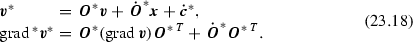
It follows that neither \({\varvec{v}}\) nor \(\mathrm {grad}\,{\varvec{v}}\) are objective quantities under Euclidian transformations. However, since \(\dot{{\varvec{O}}}^{*}{\varvec{O}}^{*\,T}\) is skew-symmetric, one obtains

.
- 5.
- 6.
The equations \({\varvec{\alpha }}({\varvec{\varXi }})=\varvec{0}\) are frequently called the Liu equations and \(\varGamma ({\varvec{\varXi }})\geqslant 0\) is the residual entropy inequality.
- 7.
The interested reader is referred to the book by Müller [24] for the explicit demonstration. One essential ingredient of the proof is that \(\varvec{\phi }\), \(\varvec{q}\), and \(\varvec{j}^{\alpha }\) are isotropic functions of their arguments. In this particular case, this is not a restriction because the chosen constitutive class (23.20) does not permit anisotropic behavior.
- 8.
For a brief biographical sketch of Josiah Willard Gibbs (1839–1903), see Fig. 17.12 in Vol. 2, p. 338 of this treatise on Fluid and Thermodynamics [22].
- 9.
If we would have written down the mass balance (23.3) for all constituents and if the mass fractions \({\xi }^{\alpha } (\alpha = 1, 2,\ldots ,N)\) for all constituents would have been used as independent constitutive variables, then instead of (23.39) one would have obtained
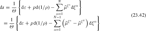
with new functions \(\bar{\mu }^{\xi ^\alpha }\); in the above expression (23.42)\(_{2}\), the relation \(\sum _{\alpha =1}^{N}\xi ^\alpha =1\) was used. Thus, one necessarily has

where the subscript in (23.43) indicates that \(\xi ^N\) is replaced by \((1- \sum _{\alpha =1}^{N-1}\xi ^\alpha )\). The variable \({\mu }^{\xi ^\alpha }\) is therefore the difference of the chemical potentials \(\left( \bar{\mu }^{\xi ^\alpha }-\bar{\mu }^{\xi ^N }\right) \), which, however, are functions of all \(\xi ^\alpha \) \((\alpha =1,2,\ldots ,N )\).
- 10.
- 11.
\(\zeta \) and \(\mu \) are the bulk and shear viscosities.
- 12.
For brief biographical sketches of Carl Ludwig (1816–1895) and Charles Soret (1854–1904), see Fig. 23.2 .
- 13.
The phenomenon is called Thermophoresis or thermodiffusion and describes the motion of suspended particles in a mixture against the temperature gradient. It can, for instance, be observed when the hot rod of an electric heater is surrounded by tobacco smoke: the smoke goes away from the immediate vicinity of the hot rod.
- 14.
This proof was not given here; it was only referred to [24], where this proof is given.
- 15.
Whereas the text of this section has independently been drafted by K. Hutter , many of the detailed arguments have been influenced by the dissertation of G. Bauer [2]. We wish to acknowledge this source, as it has also streamlined and clarified the writings at other places of this book, even though its influence may only here directly be seen.
- 16.
The true density of constituent \(\alpha \) is the mass of constituent \(\alpha \) per unit volume of this constituent (and not that of the mixture). Sometimes this is also called the apparent density.
- 17.
In classical continuum mechanics, a non-simple material is defined as a medium in which higher gradients of the motion \({\varvec{\chi }}(\varvec{X}, t)\) may arise as independent constitutive variables. This is the case, if \(\mathrm {grad}\,\rho \) is an independent constitutive variable, because \(\rho =\rho _0/\det \varvec{F}\) and therefore \(\mathrm {grad}\,\rho = \rho _0 \mathrm {grad}\,\det {\varvec{F}}^{-1}\).
- 18.
\({\varvec{U}^\alpha }\) contains symmetric and skew-symmetric contributions which can be separated into
$$ \varvec{D}^{\alpha }=\text {sym}{\varvec{U}^\alpha }= \text {sym}(\mathrm {grad}\,{\varvec{v}^\alpha }), \qquad \varvec{W}^{\alpha }=\text{ skw } \,{\varvec{U}^\alpha }= \text{ skw }(\mathrm {grad}\,{\varvec{v}^\alpha })-\varvec{W}. $$\(\varvec{D}^{\alpha }\) and \(\varvec{W}^{\alpha }\) are relative stretching and relative vorticity tensors.
- 19.
It might be worth mentioning that most authors of papers dealing with thermodynamics of solid–fluid mixtures of porous or granular materials use the second law of thermodynamics in a form akin to the Clausius–Duhem inequality with an exploitation following the Coleman–Noll procedure of exploitation. In these approaches, the balance laws of peculiar momenta and energy are associated with arbitrary source terms.
- 20.
One-form is a linear functional \({\mathcal F}\) (as a special case of multilinear functionals), in which \({\mathcal F} = \sum a_{j}\mathrm {d}x_{j}\) is a sum of finite coefficients \(a_{j}\) multiplied with differentials \(\mathrm {d}x_{j}\).
- 21.
Notice that \(\mathcal{P}_{x_i}\) and \(\mathcal{F}_{x_i}\) do not represent derivatives of \(\mathcal{P}\) and \(\mathcal{F}\), since \(\varLambda ^\varepsilon \) in (23.100) cannot be pulled into the differential of \(\rho \varepsilon \). So, neither \(\mathcal{P}\) nor \(\mathcal{F}\) are complete differentials.
- 22.
The derivation of this formidably looking inequality is not difficult, however it is lengthy and time consuming, and its derivation is susceptible to error. For this text, it was derived several times and has multiply been checked.
- 23.
With regard to the terms \(\mathcal{P}_{\nu ^\alpha }, \mathcal{P}_{\mathrm {grad}\,\nu ^\alpha } \), and \(\mathcal{F}_{\nu ^\alpha }\), the identities (23.107)\(_{3,4,7}\) are to be understood in the sense of Eq. (23.88). If \({\text {d}}\nu ^N\) should not be replaced by \(-\sum _{\alpha =1}^{N-1} {\text {d}}\nu ^\alpha \) as in (23.103), then the following substitutions should be made:
$$\begin{aligned}&\mathcal{P}_{\nu ^\alpha }-\mathcal{P}_{\nu ^N} \longrightarrow \mathcal{P}_{\nu ^\alpha }, \nonumber \\&\mathcal{P}_{\mathrm {grad}\,\nu ^\alpha }-\mathcal{P}_{\mathrm {grad}\,\nu ^N} \longrightarrow \mathcal{P}_{\mathrm {grad}\,\nu ^\alpha }, \nonumber \\&\mathcal{F}_{\mathrm {grad}\,\nu ^\alpha }-\mathcal{F}_{\mathrm {grad}\,\nu ^N} \longrightarrow \mathcal{F}_{\mathrm {grad}\,\nu ^\alpha },\nonumber \end{aligned}$$ - 24.
For a brief biographical sketch of Johann Friedrich Pfaff (1765–1825), see Fig. 17.46 in Vol. 2, p. 401 of this treatise on Fluid and Thermodynamics [22].
- 25.
For a brief biographical sketch of Josiah Willard Gibbs (1839–1903), see Fig. 17.12 in Vol. 2, p. 338 of this treatise on Fluid and Thermodynamics [22].
- 26.
In an n-dimensional space, manifolds with the dimension \(n-1\) or smaller are called hypersurfaces.
- 27.
For a brief biographical sketch of Jules Heri Poincaré (1854–1912), see Fig. 23.3 .
- 28.
For a brief biographical sketch of Ferdinand Georg Frobenius (1849–1917), see Fig. 7.31 in Vol. 1, p. 417 of this treatise on Fluid and Thermodynamics [21].
- 29.
Of the Lagrange multipliers \(\varLambda ^{\nu ^\alpha }\), only the difference \(\lambda ^{\nu ^\alpha }:= \varLambda ^{\nu ^\alpha }- \lambda ^{\nu ^N}\) can be determined. \(\lambda ^{\nu ^N}\) remains undetermined and forms an independent variable of the theory.
- 30.
This is a very natural assumption, because earlier experience has shown us that \(1/{\varLambda ^\varepsilon }\) has the meaning of absolute temperature.
- 31.
The reader may recall (23.88), which explains the peculiarities when differentiating functions (here \(\varvec{k}\)) of \(\nu ^1,\ldots ,\nu ^{N-1}\), and \(\nu ^1,\ldots ,\nu ^{N}\), respectively.
- 32.
This, for instance, excludes the situation of simultaneous existence of ice and water and mass exchanges between these two constituents as it occurs, e.g., in temperate ice. Solidification of rock or the mushy behavior of the interior core of the Earth would also be examples where such phase changes occur. This more general case is treated by Bauer [2].
- 33.
For a brief biographical sketch of Henry Philibert Gaspard Darcy (1803–1858), see Fig. 10.9 in Vol. 1, p. 594 of this treatise on Fluid and Thermodynamics [21].


References
Albers, B., Wilmanski, K.: Continuum Thermodynamics, Part II: Applications and Examples, p. 464. World Scientific, New Jersey (2015). ISBN 978-981-4412-37-7
Bauer, G.: Thermodynamische Betrachtung einer gesättigten Mischung. Doctoral dissertation, Department of Mechanics, Darmstadt University of Technology, 126p. (1997)
Biot, M.A.: General theory of three dimensional consolidation. J. Appl. Phys. 12, 155–164 (1941)
Biot, M.A.: Theory of deformation of a porous viscoelastic anisotropic solid. J. Appl. Phys. 27, 459–467 (1956)
Bluhm, J.: A Consistent Model for Saturated and Empty Porous Media. Forschungsberichte aus dem Fachbereich Bauwesen, vol. 74, p. 133p. Universität GH Essen, Essen (1997)
Bowen, R.M.: Incompressible porous media models by use of the theory of mixtures. Int. J. Eng. Sci. 18, 1129–1148 (1980)
Bowen, R.M.: Compressible porous media models by use of the theory of mixtures. Int. J. Eng. Sci. 20, 697–763 (1982)
Bowen, R.M., Wang, C.-C.: Introduction to Vectors and Tensors. Vol. 1: Linear and Multillinear Algebra, pp. 1–296; Vol. 2: Vector and Tensor Analysis, pp. 297–520. Plenum Press (1976)
de Boer, R.: Theory of Porous Media. Highlights in the Historical Development and Current State, 618p. Springer, Berlin (2000)
Drew, D.A., Passman, S.L.: Theory of Multicomponent Fluids. Applied Mathematical Sciences, vol. 135l, 308p. Springer, New York (1998)
Ehlers, W.: Poröse Medien – Ein kontinuumsmechanisches Model auf der Basis der Mischungstheorie. Forschungsberichte aus dem Fachbereich Bauwesen, vol. 47, 322p. Universität GH Essen, Essen (1989)
Ehlers, W.: Constitutive equations for granular materials in geomechanical context. In: Hutter, K. (ed.) Continuum Mechanics in Environmental Sciences and Geophysics. CISM Courses and Lectures, vol. 337, pp. 313–402. Springer, Vienna (1993)
Goodman, M.A., Cowin, S.C.: A continuum theory of granular materials. Arch. Ration. Mech. Anal. 44, 249–266 (1972)
Gray, W.G.: Elements of a systematic procedure for the derivation of macroscale conservation equations for multiphase flows in porous media. In: Hutter, K. (ed.) Kinematic and Continuum Theories of Granular and Porous Media. CISM Courses and Lectures, vol. 400, pp. 67–129. Springer, Berlin (1999)
Gray, W.G., Miller, C.T.: Introduction to the thermodynamically constrained averaging theory for porous media systems. In: Hutter, K. (ed.) Advances in Geophysical and Environmental Mechanics and Mathematics (AGEM\(^{2}\)). Springer, Cham (2014)
Gurtin, M.E.: On the thermodynamics of chemically reacting fluid mixtures. Arch. Ration. Mech. Anal. 43, 198–212 (1971)
Hassaniazadeh, S.M., Gray, W.G.: General conservation equations for multiphase systems: 1. Averaging procedure. Adv. Water Res. 2, 25–40 (1979)
Hassaniazadeh, S.M., Gray, W.G.: General conservation equations for multiphase systems: 1. Averaging procedure. Adv. Water Res. 2, 131–144 (1979)
Hassaniazadeh, S.M., Gray, W.G.: General conservation equations for multiphase systems: 2. Mass, momenta, energy and entropy equations. Adv. Water Res. 2, 191–208 (1979)
Hutter, K., Jöhnk, K.: Continuum Methods of Physical Modeling, p. 635. Springer, Berlin (2004)
Hutter, K., Wang, Y.: Fluid and Thermodynamics. Volume 1: Basic Fluid Mechanics, 639p. Springer, Berlin (2016). ISBN: 978-3319336329
Hutter, K., Wang, Y.: Fluid and Thermodynamics. Volume II: Advanced Fluid Mechanics and Thermodynamic Fundamentals. Springer, Berlin, 633p. (2016). ISBN: 978-3-319-33635-0
Ludwig, C.: Diffusion zwischen ungleich erwärmten Orten gleich zusammengesetzter Lösungen. Sitzungsbericbht Kaiser. Akad. Wiss. (Mathem-Naturwiss. Cl.) Wien, 65, 539 (1856)
Müller, I.: Thermodynamics. Pitman, 521p. (1985)
Schneidere, L., Hutter, K.: Solid-fluid mixtures of frictional materials in geophysical and geotechnical context. In: Hutter, K. (ed.) Advances in Geophysical and Environmental Mechanics and Mathematics (AGEM\(^{2}\)), p. 247. Springer, Berlin (2009)
Soret, C.: Sur l’état d‘ équilibre que prend, du point de vue de sa concentration, une dissolution saline primitivement homogéne, dont deux parties sont portées à des tempéeratures difféerantes. Archives de Genève, 3e période, tome II, 48 (1879)
Svendsen, B., Hutter, K.: On the thermodynamics of a mixture of isotropic viscous materials with kinematic constraints. Int. J. Eng. Sci. 33, 2021–2054 (1995)
Truesdell, C.A., Toupin, R.A.: The classical field theories. In: Flügge, S. (ed.) Encyclopedia of Physics, vol. III/1, pp. 226–793. Springer, Berlin (1957)
Truesdell, C.A.: Essays in the History of Mechanics, 383p. Springer, Berlin (1968)
Truesdell, C.A.: Rational Thermodynamics, 2nd edn, 578p. Springer, Berlin (1984)
Wilmanski, K.: Continuum Thermodynamics, Part I: Foundations, p. 402. Wold Scientific, Singapore (2008). ISBN 978-981-283-556-7
Author information
Authors and Affiliations
Corresponding author
Appendices
Appendix 23.A Some Details on the Poincaré Theorem and the Condition of Frobenius
In this appendix, we shall prove the correctness of the following statements:
Proposition 23.4
-
(i)
In the one-dimensional case (\(n = 1\)) every total differential is complete.
-
(ii)
In two dimensions (\(n = 2\)), every differential can be transformed into a total differential by multiplying it with an integrating factor.
-
(iii)
In three-dimensional space (\(n = 3\)), the condition that an arbitrary differential \(\mathrm {d}F = X_{i}\mathrm {d}x_{i}\) can be made complete is the requirement that the vector field \({\varvec{X}}\) stays perpendicular to its vorticity, \(\mathrm {curl}\,{\varvec{X}}\). \(\blacksquare \)
Proof
-
(i)
In the one-dimensional case, there is no possibility to select between different paths of integration between two points to reach point b from point a. Every Riemann integral from a to a certainly vanishes.
-
(ii)
In two dimensions, one has \(\mathrm {d}F = X_{1}\mathrm {d}x_{1} + X_{2}\mathrm {d}x_{2}\). If Poincaré’s theorem holds, then
$$\begin{aligned} \frac{\partial X_{1}}{\partial x_{2}} = \frac{\partial X_{2}}{\partial x_{1}} \end{aligned}$$(23.174)and F is a potential such that
$$\begin{aligned} X_{1} = \frac{\partial F}{\partial x_{1}}, \quad X_{2} = \frac{\partial F}{\partial x_{2}} \quad {\mathop {\Longrightarrow }\limits ^{(23.147)}} \quad \frac{\partial ^{2}F}{\partial x_{2}\partial x_{1}} = \frac{\partial ^{2}F}{\partial x_{1}\partial x_{2}}. \end{aligned}$$(23.175)The value \(F({\varvec{x}})\) can be determined by integrating from \({\varvec{x}_{0}}\) to \({\varvec{x}}\) along any continuous curve,
$$\begin{aligned} F({\varvec{x}}) = \int _{{\varvec{x}}_{0}}^{{\varvec{x}}}\left( X_{1}(x_{1}, x_{2})\mathrm {d}x_{1} + X_{2}(x_{1}, x_{2})\mathrm {d}x_{2}\right) . \end{aligned}$$(23.176)It follows that the integral along any curve from \({\varvec{a}}\) to \({\varvec{b}}\) yields
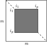
$$\begin{aligned} \int _{{\varvec{a}}}^{{\varvec{b}}}\left( X_{1}(x_{1}, x_{2})\mathrm {d}x_{1} + X_{2}(x_{1}, x_{2})\mathrm {d}x_{2}\right) = \int _{{\varvec{a}}}^{{\varvec{b}}}\mathrm {d}F = F({\varvec{b}}) - F({\varvec{a}})\quad \end{aligned}$$(23.177)and is independent of the path chosen between \({\varvec{a}}\) and \({\varvec{b}}\), see Fig. 23.4 .

Explaining the path independence of the integration of a differential in two dimensions
If the Poincaré theorem is not fulfilled, one may try its satisfaction by an integrating factor. In that case, one writes
Satisfaction of the Poincaré theorem for this differential requires
in which the underbraced term differs from zero since the starting equation does not satisfy the Poincaré condition. Evidently, \(\lambda = \mathrm {const.}\) is not a possible integrating factor. However, the determination of a nonconstant integrating factor is not unique.
-
If \(X_{2} \ne 0\), one may, for instance, select \(\lambda = \lambda _{1}(x_{1})\); then it follows from (23.180) that
 (23.181)
This formula shows that \(\lambda _{1}\) is a function of \(x_{1}\) alone only, if the integrand function is independent of \(x_{2}\)
-
If \(X_{1} \ne 0\) and \(\lambda = \lambda _{2}(x_{2})\) is assumed, the analogous procedure leads to
 (23.182)
which shows that \(\lambda = \lambda _{2}(x_{2})\) is only a function of \(x_{2}\), if the integrand function does not depend on \(x_{1}\).
-
In all other cases, \(\lambda \) must be determined by solving the partial differential equation (23.180).


-
(iii)
In the three-dimensional case, it is known that a vector field \({\varvec{X}}\) can be written as the gradient of a scalar potential field only, if \(\mathrm {curl}\,{\varvec{X}} = {\varvec{0}}\). In Cartesian component form, this then yields the Poincaré condition
$$\begin{aligned} \frac{\partial X_{i}}{\partial x_{j}} - \frac{\partial X_{j}}{\partial x_{i}} = 0, \quad (i, j = 1, 2, 3). \end{aligned}$$If \(\mathrm {curl}\,{\varvec{X}} \ne {\varvec{0}}\), one may try to construct a total differential
$$\begin{aligned} \mathrm {d}F_{\lambda } = \lambda X_{1}\mathrm {d}x_{1} + \lambda X_{2}\mathrm {d}x_{2} + \lambda X_{3}\mathrm {d}x_{3}, \end{aligned}$$(23.183)by multiplying \(\mathrm {d}F\) with an integrating factor. The condition for this to be successful is
$$\begin{aligned} {\varvec{0}} {\mathop {=}\limits ^{!}} \mathrm {curl}\,(\lambda {\varvec{X}}) = \lambda (\mathrm {curl}\,{\varvec{X}}) + (\mathrm {grad}\,\lambda )\times {\varvec{X}}. \end{aligned}$$(23.184)Multiplying this equation scalarly with \({\varvec{X}}\) yields
$$\begin{aligned} \mathrm {curl}\,{\varvec{X}}\cdot {\varvec{X}} = 0, \quad \mathrm {if}\; \lambda \ne 0. \end{aligned}$$(23.185)Thus, \({\varvec{X}}\) and \(\mathrm {curl}\,{\varvec{X}}\) are perpendicular to one another; in Cartesian components, this reads
$$\begin{aligned} \varepsilon _{ijk}X_{k,j}X_{i} = 0, \end{aligned}$$(23.186)which is nothing else than the Frobenius condition.
For a plane vector field, condition (23.185) is always satisfied; a fact that corroborates the statement that in two dimensions an integrating factor always exists.
Appendix 23.B Proof of a Statement About a Complete Differential
In this Appendix, the following statement is proved:
Let \(\mathrm {d}f\) be an incomplete differential of the variables \(x_{i}\) \((i=1,\ldots ,n)\). Let, moreover, \(g \ne 0\) be an integrating denominator, which makes
a total (complete) differential. Then,
is equally complete.
Proof
In long-hand notation, \(\mathrm {d}H\) is written as
Hence,
Testing Poincaré’s theorem, one deduces,
In these expressions, the second terms are equal, because, by prerequisite, \(\mathrm {d}f/g\) is a complete differential (Poincaré theorem). This is also true for the first term, since according to (23.187)
It has, therefore, been proved that the two mixed derivatives (23.191) have the same value. It follows that \(\mathrm {d}H\) is necessarily a complete differential, if \(\mathrm {d}F\) is one.
Appendix 23.C Proof of Some Rules of Differentiation
-
(i)
The formulae (23.95)\(_{1,2,3}\) follow from the definition of the barycentric velocity, \({\varvec{v}}=\sum _{\gamma =1}^{N}\xi ^{\gamma }{\varvec{v}}^{\gamma } \) by applying the product rule of differentiation. For instance,
$$\begin{aligned} \mathrm {grad}\,{\varvec{v}} = \sum _{\gamma =1}^{N}\left\{ \xi ^{\gamma }\mathrm {grad}\,{\varvec{v}}^{\gamma } + {\varvec{v}}^{\gamma }\otimes \mathrm {grad}\,\xi ^{\gamma }\right\} , \end{aligned}$$(23.193)from which expressions for \({\varvec{D}}\) and \({\varvec{W}}\) may be derived by applying the operators “sym” and “skw”,
$$\begin{aligned} {\varvec{D}}= & {} \sum _{\gamma =1}^{N}\left\{ \xi ^{\gamma }{\varvec{D}}^{\gamma } + \mathrm {sym} \left( {\varvec{v}}^{\gamma }\otimes \mathrm {grad}\,\xi ^{\gamma }\right) \right\} , \nonumber \\[-2.5mm] \\[-2.5mm] {\varvec{W}}= & {} \sum _{\gamma =1}^{N}\left\{ \xi ^{\gamma }{\varvec{W}}^{\gamma } + \mathrm {skw}\left( {\varvec{v}}^{\gamma }\otimes \mathrm {grad}\,\xi ^{\gamma }\right) \right\} . \nonumber \end{aligned}$$(23.194) -
(ii)
From the definition of the diffusion velocity, there follows
$$\begin{aligned} \frac{\partial {\varvec{u}}^{\beta }}{\partial {\varvec{v}}^\alpha } = \frac{\partial }{\partial {\varvec{v}}^{\alpha }} \left( {\varvec{v}}^{\beta } - \sum _{\gamma =1}^{N}\xi ^{\gamma }{\varvec{v}}^{\gamma }\right) = \delta _{\alpha \beta } {\varvec{I}} - \xi ^{\alpha }{\varvec{I}} = \left( \delta _{\alpha \beta } - \xi ^{\alpha }\right) {\varvec{I}},\qquad \end{aligned}$$(23.195)in which \({\varvec{I}}\) is the \(3\times 3\) unit rank-2 tensor. Similarly,
$$\begin{aligned} \frac{\partial {\varvec{U}}^{\beta }}{\partial {\varvec{W}}^{\alpha }}= & {} \frac{\partial }{\partial {\varvec{W}}^\alpha }\left\{ \mathrm {grad}\,{\varvec{v}}^{\beta } - \sum _{\gamma =1}^{N}\left( \xi ^{\gamma }{\varvec{W}}^{\gamma } + \mathrm {skw}\left( {\varvec{v}}^{\gamma }\otimes \mathrm {grad}\,\xi ^{\gamma }\right) \right) \right\} \nonumber \\= & {} \delta _{\alpha \beta }{\varvec{I}}_{4}-\xi ^{\alpha }{\varvec{I}}_{4} = \left( \delta _{\alpha \beta }- \xi ^{\alpha }\right) {\varvec{I}}_{4}, \end{aligned}$$(23.196)in which \({\varvec{I}}_{4}\) is the unit rank-4 tensor with \(({\varvec{I}}_{4})_{ijkl} = \delta _{ij}\delta _{kl}\).
-
(iii)
With the results (23.195) and (23.196), we may now deduce
$$\begin{aligned} \frac{\partial f}{\partial {\varvec{v}}^{\alpha }}= & {} \sum _{\beta }\frac{\partial f}{\partial {\varvec{u}}^{\beta }} \frac{\partial {\varvec{u}}^{\beta }}{\partial {\varvec{v}}^{\alpha }} =\sum _{\beta }\frac{\partial f}{\partial {\varvec{u}}^{\beta }}\left( \delta _{\alpha \beta } - \xi ^{\alpha }\right) {\varvec{I}} \nonumber \\= & {} \frac{\partial f}{\partial {\varvec{u}}^{\alpha }} - \xi ^{\alpha }\sum _{\beta } \frac{\partial f}{\partial {\varvec{u}}^{\beta }}, \end{aligned}$$(23.197)$$\begin{aligned} \frac{\partial f}{\partial {\varvec{W}}^{\alpha }}= & {} \sum _{\beta }\frac{\partial f}{\partial {\varvec{U}}^{\beta }}\frac{\partial {\varvec{U}}^{\beta }}{\partial {\varvec{W}}^{\alpha }} = \sum _{\beta } \frac{\partial f}{\partial {\varvec{U}}^{\beta }}\left( \delta _{\alpha \beta } - \xi ^{\alpha }\right) {\varvec{I}}_{4} \nonumber \\= & {} \frac{\partial f}{\partial {\varvec{U}}^{\alpha }} - \xi ^{\alpha }\sum _{\beta }\frac{\partial f}{\partial {\varvec{U}}^{\beta }}. \end{aligned}$$(23.198)This result can now be used in the evolution of \(\partial f/\partial \mathrm {grad}\,{\varvec{v}}^{\alpha }\)
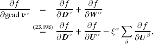 (23.199)

where \(\mathrm {grad}\,{\varvec{v}}^{\alpha } = {\varvec{D}}^{\alpha } + {\varvec{W}}^{\alpha }\) has been used.
Rights and permissions
Copyright information
© 2018 Springer International Publishing AG, part of Springer Nature
About this chapter

Cite this chapter
Hutter, K., Wang, Y. (2018). Thermodynamics of Class I and Class II Classical Mixtures. In: Fluid and Thermodynamics. Advances in Geophysical and Environmental Mechanics and Mathematics. Springer, Cham. https://doi.org/10.1007/978-3-319-77745-0_23
Download citation
DOI: https://doi.org/10.1007/978-3-319-77745-0_23
Published:
Publisher Name: Springer, Cham
Print ISBN: 978-3-319-77744-3
Online ISBN: 978-3-319-77745-0
eBook Packages: Earth and Environmental ScienceEarth and Environmental Science (R0)