
Abstract
Recently, Döttling and Garg (CRYPTO 2017) showed how to build identity-based encryption (IBE) from a novel primitive termed Chameleon Encryption, which can in turn be realized from simple number theoretic hardness assumptions such as the computational Diffie-Hellman assumption (in groups without pairings) or the factoring assumption. In a follow-up work (TCC 2017), the same authors showed that IBE can also be constructed from a slightly weaker primitive called One-Time Signatures with Encryption (OTSE).
In this work, we show that OTSE can be instantiated from hard learning problems such as the Learning With Errors (LWE) and the Learning Parity with Noise (LPN) problems. This immediately yields the first IBE construction from the LPN problem and a construction based on a weaker LWE assumption compared to previous works.
Finally, we show that the notion of one-time signatures with encryption is also useful for the construction of key-dependent-message (KDM) secure public-key encryption. In particular, our results imply that a KDM-secure public key encryption can be constructed from any KDM-secure secret-key encryption scheme and any public-key encryption scheme.
Research supported in part from 2017 AFOSR YIP Award, DARPA/ARL SAFEWARE Award W911NF15C0210, AFOSR Award FA9550-15-1-0274, NSF CRII Award 1464397, and research grants by the Okawa Foundation, Visa Inc., and Center for Long-Term Cybersecurity (CLTC, UC Berkeley). The views expressed are those of the author and do not reflect the official policy or position of the funding agencies.
You have full access to this open access chapter, Download conference paper PDF
1 Introduction
Identity-based encryption (IBE) is a form of public key encryption that allows a sender to encrypt messages to a user without knowing a user-specific public key, but only the user’s name or identity and some global and succinct public parameters. The public parameters are issued by a key authority which also provides identity-specific secret keys to the users.
The notion of IBE was originally proposed by Shamir [Sha84], and in two seminal results Boneh and Franklin [BF01] and Cocks [Coc01] provided the first candidate constructions of IBE in the random oracle model from groups with pairings and the quadratic residue problem respectively. Later works on IBE provided security proofs without random oracles [CHK04, BB04, Wat05, Wat09, LW10, BGH07] and realized IBE from hard lattice problems [GPV08, CHKP12, ABB10].
In a recent result, Döttling and Garg [DG17b] showed how to construct IBE from (presumably) qualitatively simpler assumptions, namely the computational Diffie-Hellman assumption in groups without pairings or the factoring assumption. In a follow-up work, the same authors [DG17a] provided a generalization of the framework proposed in [DG17b]. In particular, the authors show that identity-based encryption is equivalent to the seemingly simpler notion of One-Time Signatures with Encryption (OTSE) using a refined version of the tree-based IBE construction of [DG17b].
An OTSE-scheme is a one-time signature scheme with an additional encryption and decryption functionality. Informally, the encryption functionality allows anyone to encrypt a plaintext \(\mathsf {m} \) to a tuple consisting of a public parameter \(\mathsf {pp}\), a verification key \(\mathsf {vk} \), an index i and a bit b, to obtain a ciphertext \(\mathsf {c} \). The plaintext \(\mathsf {m} \) can be deciphered from \(\mathsf {c} \) by using a pair of message-signature \((\mathsf {x}, \sigma )\) that is valid relative to \(\mathsf {vk} \) and which satisfies \(\mathsf {x} _i = b\). Security of the OTSE asserts that an adversary knowing a pair of message-signature \((\mathsf {x}, \sigma )\) and the underlying public parameter \(\mathsf {pp}\) and verification key \(\mathsf {vk} \) cannot distinguish between encryptions of two plaintexts encrypted to \((i, 1-\mathsf {x} _i)\) under \((\mathsf {pp}, \mathsf {vk})\), for any index i of the adversary’s choice. (Note that this security property implies the one-time unforgeability of the signature.) The OTSE also needs to be compact, meaning the size of the verification key grows only with the security parameter, and does not depend on the size of messages allowed to be signed.
1.1 PKE and IBE from Learning with Errors
We will briefly review constructions of public-key encryption and identity-based encryption from the Learning with Errors (LWE) problem.
The hardness of LWE is determined by its dimension n, modulus q, noise magnitude parameter \(\alpha \) and the amount of samples m. Regev [Reg05] showed that among the latter three parameters, in particular the noise magnitude parameter \(\alpha \) is of major importance since it directly impacts the approximation factor of the underlying lattice problem.
Theorem 1
[Reg05]. Let \(\epsilon =\epsilon (n)\) be some negligible function of n. Also, let \(\alpha =\alpha (n)\in (0,1)\) be some real and let \(p=p(n)\) be some integer such that \(\alpha p>2\sqrt{n}\). Assume there exists an efficient (possibly quantum) algorithm that solves LWE\(_{p,\alpha }\). Then there exists an efficient quantum algorithm for solving the following worst-case lattice problems:
-
1.
Find a set of n linearly independent lattice vectors of length at most \(\tilde{O}(\lambda _n(L)\cdot n/\alpha )\).
-
2.
Approximate \(\lambda _1(L)\) within \(\tilde{O}(n/\alpha )\).
Here, \(\lambda _k\) is the minimal length of k linearly independent vectors in lattice L. To find such vectors within a constant or slightly sublinear approximation is known to be NP-hard under randomized reductions [ABSS93, Ajt98, Mic98, Kho04, HR07], while for an exponential approximation factor, they can be found in polynomial time using the LLL algorithm [LLL82]. Regev [Reg05] introduced the first PKE based on LWE for a choice of \(\alpha =\tilde{O}(1/\sqrt{n})\), more precisely \(\alpha =1/(\sqrt{n}\log ^2 n)\). The first lattice based IBEs, by Gentry et al. [GPV08], Cash et al. [CHKP10] and by Agrawal et al. [ABB10] require \(\alpha =\tilde{O}(1/n)\), \(\alpha =\tilde{O}(1/(\sqrt{k}n))\), where k is the output length of a hash function, and \(\alpha =\tilde{O}(1/n^2)\).
The reason for this gap between PKE and IBE is that all the known IBE constructions use an additional trapdoor in order to sample short vectors as secret keys. This sampling procedure increases the norm of sampled vectors, such that the initial noise of a ciphertext must be decreased to maintain the correctness of the schemes. By losing a factor \(\sqrt{n}\) in the sampling procedure [MR04, GPV08, MP12, LW15], \(\alpha \) needs to be chosen by a factor \(\sqrt{n}\) smaller. Therefore, this methodology unavoidably loses at least an additional \(\sqrt{n}\) factor. This explains why these techniques cause a gap compared to Regev’s PKE where \(\alpha \) is at least a factor \(\sqrt{n}\) larger, which decreases the approximation factor by at least a factor of \(\sqrt{n}\). This results in a stronger assumption with respect to the underlying short vector problem.
1.2 Our Results
As the main contribution of this work, we remove the requirement of the collision-tractability property of the hash function in the construction of [DG17a]. Specifically, we replace the notion of Chameleon Encryption with the simpler notion of Hash Encryption, for which no collision tractability property is required. The notion of Hash Encryption naturally arises from the notion of laconic Oblivious Transfer [CDG+17]. We provide simple and efficient constructions from the Learning With Errors (LWE) [Reg05] and (exponentially hard) Learning Parity with Noise (LPN) problem [YZ16].
Our overall construction of IBE from hash encryption proceeds as follows. We first show that we can use any CPA PKE to build a non-compact version of One-Time Signatures with Encryption (OTSE), in which, informally, the size of the verification key of the OTSE is bigger than the size of the messages allowed to be signed. We then show how to use hash encryption to boost non-compact OTSE into compact OTSE, under which arbitrarily large messages could be signed using a short public parameter and a short verification key, while preserving the associated encryption-decryption functionalities. Our transformation makes a non-black-box use of the non-compact OTSE primitive.
Using a recent result by Döttling and Garg [DG17a], we transform our compact OTSE to an IBE. Hence, we obtain the first constructions of IBE from the LWE assumption used by Regev’s PKE and the first construction from an LPN problem.
Further, we show how to use non-compact OTSE to transform key-dependent-message (KDM) secure private key encryption to KDM-secure public key encrpyption. Informally, a private-key encryption scheme is \(\mathcal {F}\)-KDM secure, for a function class \(\mathcal {F}\), if the scheme remains semantically secure even if the adversary is allowed to obtain encryptions of \(f(\mathsf {k})\), for \(f \in \mathcal {F}\), under the secret key \(\mathsf {k} \) itself. This notion is analogously defined for PKE. A large body of work, e.g., [BHHO08, ACPS09, BG10, BHHI10, App14, Döt15], shows how to build KDM-secure schemes from various specific assumptions. Briefly, in order to construct KDM-secure schemes for a large class of functions, they first show how to build KDM-secure schemes for a basic class of functions [BHHO08, BG10, ACPS09] (e.g., projections, affine) and then use KDM amplification procedures [BHHI10, App14] to obtain KDM security against richer functions families. We show that for any function family \(\mathcal {F}\), an \(\mathcal {F}\)-KDM secure PKE can be obtained from a non-compact OTSE (and hence a CPA PKE) together with a \(\mathcal {G}\)-KDM secure private-key encryption scheme, where \(\mathcal {G}\) is a class of functions related to \(\mathcal {F}\). (See Sect. 6 for a formal statement.) Using the result of [App14] we obtain that \(\mathcal {F}\)-KDM-secure PKE, for any \(\mathcal {F}\), can be based on projection-secure private-key encryption and CPA PKE. We mention that prior to our work it was not known whether projection-secure PKE (which is sufficient for KDM PKE) could be constructed (in a black-box or a non-black-box way) from the combination of CPA PKE and projection-secure private-key encryption.
An overview of the contributions of this work is given in Fig. 1.

Overview of the results in this work, bold arrows are contributions of this work.
1.3 Technical Outline
We will start by providing an outline of our construction of hash encryption from LWE. The LPN-based construction is similar in spirit, yet needs to account for additional subtleties that arise in the modulus 2 case. We will then sketch our construction of IBE from hash encryption.
Hash Encryption from LWE. The hashing key \(\mathsf {k} \) of our hash function is given by a randomly chosen matrix \(A \leftarrow {\mathbb Z}^{m \times \kappa }_p\). To hash a message, we encoded it as a vector \(\mathsf {x} \in \{0,1\}^{m} \subseteq {\mathbb Z}^{m}\) and compute the hash value \(\mathsf {h} \leftarrow \mathsf {x} ^\top \cdot A\). It can be shown that under the short integer solution (SIS) problem [Reg05] this function is collision resistant.
We will now specify the encryption and decryption procedures. Our encryption scheme is a variant of the dual-Regev [GPV08] encryption scheme. For a matrix A, let \(A_{-i}\) denote the matrix obtained by removing the i-th row of A, and let \(a_i\) be the i-th row of A. Likewise, for a vector \(\mathsf {x} \) let \(\mathsf {x} _{-i}\) denote the vector obtained by dropping the i-th component of \(\mathsf {x} \). Given the hashing key \(\mathsf {k} = A\), a hash-value \(\mathsf {h} \), an index i and a bit b, we encrypt a message \(\mathsf {m} \in \{0,1\}\) to a ciphertext \(\mathsf {c} = (c_1,c_2)\) via
where \(s \leftarrow {\mathbb Z}_p^{\kappa }\) is chosen uniformly at random and \(e \in {\mathbb Z}_p^{m}\) is chosen from an appropriate discrete gaussian distribution.
To decrypt a ciphertext \(\mathsf {c} \) using a preimage \(\mathsf {x} \), compute
output 0 if \(\mu \) is closer to 0 and 1 if \(\mu \) is closer to p/2. Correctness of this scheme follows similarly as in the dual Regev scheme [GPV08]. To argue security, we will show that a successful adversary against this scheme can be used to break the decisional extended LWE problem [AP12], which is known to be equivalent to standard LWE.
Compact OTSE from Non-compact OTSE and Hash Encryption. To obtain a compact OTSE scheme, we hash the verification keys of the non-compact OTSE-scheme using the hash function of the hash encryption primitive. While this resolves the compactness issue, it destroys the encryption-decryption functionalities of the non-compact OTSE. We overcome this problem through a non-blackbox usage of the encryption function of the base non-compact OTSE-scheme.
KDM Security. We sketch the construction of a \(\mathsf {KDM}^{\mathsf {CPA}}\)-secure PKE from a non-compact OTSE \(\mathsf {NC}\) and a \(\mathsf {KDM}^{\mathsf {CPA}}\)-secure secret-key encryption scheme \(\mathsf {SKE}= (\mathsf {Enc},\mathsf {Dec})\). We also need a garbling scheme \((\mathsf {Garble},\mathsf {Eval})\), which can be built from \(\mathsf {SKE}\).
The public key \(\mathsf {pk} = (\mathsf {pp}, \mathsf {vk})\) of the PKE is a public parameter \(\mathsf {pp}\) and a verification key \(\mathsf {vk} \) of \(\mathsf {NC}\) and the secret key is \( \mathsf {sk} = (\mathsf {k}, \sigma )\), where \(\mathsf {k}\) is a key of the secret-key scheme and \(\sigma \) is a valid signature of \(\mathsf {k}\) w.r.t. \(\mathsf {vk} \).
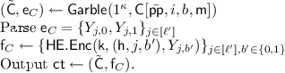
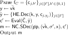
To encrypt \(\mathsf {m} \) under \(\mathsf {pk} = (\mathsf {pp}, \mathsf {vk})\) we first form a circuit \(\mathsf {C} \) which on input \(\mathsf {k}'\) returns \(\mathsf {Enc} (\mathsf {k}', m)\). We then garble \(\mathsf {C} \) to obtain a garbled circuit \(\tilde{\mathsf {C}}\) and input labels \((X_{\iota ,0}, X_{\iota ,1})\) for every input index \(\iota \). For all \(\iota \) and bit b, we OTSE-encrypt \(X_{\iota ,b}\) relative to the index \(\iota \) and bit b (using \(\mathsf {pp}\) and \(\mathsf {vk} \)) to get \(\mathsf {ct} _{\iota , b}\). The resulting ciphertext is then \(\mathsf {ct} = (\tilde{\mathsf {C}}, \{ \mathsf {ct} _{\iota , b} \}_{\iota , b} )\).
For decryption, using \((\mathsf {k}, \sigma )\) we can OTSE-decrypt the proper \(\mathsf {ct} _{\iota , b}\)’s to obtain a matching garbled input \(\tilde{\mathsf {k}}\) for \(\mathsf {k}\). Then evaluating \(\tilde{\mathsf {C}}\) on \(\tilde{\mathsf {k}}\) we obtain \(\mathsf {ct} ' = \mathsf {Enc} (k, m)\). We can then decrypt \(\mathsf {ct} '\) using \(\mathsf {k}\) to recover \(\mathsf {m} \).
Using a series of hybrids we reduce the KDM security of the PKE to the stated security properties of the base primitives.
1.4 Concurrent Works
In a concurrent and independent work, Brakerski et al. [BLSV17] provided a construction of an IBE scheme from \(\mathsf {LPN}\) with a very low noise rate of \(\varOmega (\log (\kappa )^2/\kappa )\), using techniques similar to the construction of OTSE from sub-exponentially hard \(\mathsf {LPN}\) in this work. Also in a concurrent and independent work, Kitagawa and Tanaka [KT17] provided a construction of KDM-secure public key encryption from KDM-secure secret key encryption and IND-CPA secure public key encryption using techniques similar to ours.
2 Preliminaries
We use \(\{0,1\}^{m}_k\) to denote the set of binary vectors of length \(m \) with hamming weight k and [m] to denote the set \(\{1,\ldots ,m\}\). We use \(A_{-i}\) to denote matrix A where the ith row is removed. The same holds for a row vector \(\mathsf {x} _{-i}\), which denotes vector \(\mathsf {x} \) where the ith entry is removed.
Lemma 1
For \(m \in {\mathbb N}\) and \(1\le k\le m \), the cardinality of set \(\{0,1\}^{m}_k\) is lower bounded by \(\big (\frac{m}{k}\big )^k\) and upper bounded by \(\big (\frac{em}{k}\big )^k\).
Definition 1
(Bias). Let \(x \in {\mathbb F}_2\) be a random variable. Then the bias of x is defined by
Remark 1
The bias of x is simply the second Fourier coefficient of the probability distribution of x, the first Fourier coefficient being 1 for all distributions. Thus, as \(\Pr [x = 1] = 1 - \Pr [x = 0]\) it holds that \(\Pr [x = 0] = \frac{1}{2} + \frac{1}{2}\mathsf {bias} (x)\).
In the following, we summarize several useful properties of the bias of random variables.
-
If \(x \leftarrow B _\rho \), then \(\mathsf {bias} (x) = 1 - 2\rho \).
-
Let \(x_1,x_2 \in {\mathbb F}_2\) be independent random variables. Then it holds that \(\mathsf {bias} (x_1 + x_2) = \mathsf {bias} (x_1) \cdot \mathsf {bias} (x_2)\).
-
Assume that the distribution of x is the convex combination of two distributions via \(p_x = \alpha p_{x_1} + (1 - \alpha ) p_{x_2}\). Then \(\mathsf {bias} (x) = \alpha \mathsf {bias} (x_1) + (1 - \alpha ) \mathsf {bias} (x_2)\).
Proof
Convolution theorem
Lemma 2
Let \(v \in {\mathbb F}_2^n\) be a vector of weight t and \(e \in {\mathbb F}_2^n\) a distribution for which each component is iid distributed with bias \(\epsilon \). Then it holds that \(\Pr [\langle v, e \rangle = 0] = \frac{1}{2} + \frac{1}{2} \epsilon ^t\).
Proof
As v has weight t, it holds that
where the second equality follows by the properties of the bias. Consequently, it holds that \(\Pr [\langle v, e \rangle = 0] = \frac{1}{2} + \frac{1}{2} \epsilon ^t\). \(\square \)
2.1 Hard Learning Problems
We consider variants of the learning problems \(\mathsf {LWE}\) and \(\mathsf {LPN}\) that are known to be as hard as the original problems. These variants are called extended \(\mathsf {LWE}\) or \(\mathsf {LPN}\), since they leak some additional information about the noise term.
Definition 2
(Extended LWE). A ppt algorithm \(\mathcal {A} =(\mathcal {A} _1,\mathcal {A} _2)\) breaks extended \(\mathsf {LWE}\) for noise distribution \(\varPsi \), \(m\) samples, modulus p and dimension \(\kappa \) if
where \((x,\mathsf {st})\leftarrow \mathcal {A} _1(1^\kappa )\) and the randomness is taken over \(A\leftarrow {\mathbb Z}_p^{m \times \kappa }\), \(B\leftarrow {\mathbb Z}_p^{m}\), \(s\leftarrow {\mathbb Z}_p^\kappa \), \(e\leftarrow \varPsi \) and a non-negligible \(\epsilon \).
Lemma 3
[AP12, Theorem 3.1]. For dimension \(\kappa \), modulus q with smallest prime divisor p, \(m\ge \kappa +\omega (\log (\kappa ))\) samples and noise distribution \(\varPsi \), if there is an algorithm solving extended \(\mathsf {LWE}\) with probability \(\epsilon \), then there is an algorithm solving \(\mathsf {LWE}\) with advantage \(\frac{\epsilon }{2p-1}\) as long as p is an upper bound on the norm of the hint \(x^Te\).
When \(p=2\) and the noise distribution \(\varPsi = B _\rho \) is the Bernoulli distribution, we call the problem \(\mathsf {LPN}\). The \(\mathsf {LPN}\) problem was proposed by [BFKL94] for the private key setting. A series of works [Ale03, DMQN12, KMP14, Döt15] provided public key encryption schemes from the so-called low-noise \(\mathsf {LPN}\) problem where the error term has a noise-rate of \(O(1/\sqrt{\kappa })\). In a recent work, Yu and Zhang [YZ16] provided public key encryption schemes based on \(\mathsf {LPN}\) with a constant noise-rate but a sub-exponential number of samples \(m = 2^{O(\sqrt{\kappa })}\). We refer to this variant as (sub-) exponentially hard \(\mathsf {LPN}\).
For our \(\mathsf {LPN}\) based encryption scheme, we need to be able to embed a sufficiently strong binary error correction code such that decryption can recover a message. Therefore, we define a hybrid version of extended \(\mathsf {LPN}\) that is able to hide a sufficiently large generator matrix of such a code.
Definition 3
(Extended Hybrid LPN). A ppt algorithm \(\mathcal {A} =(\mathcal {A} _1,\mathcal {A} _2)\) breaks extended \(\mathsf {LPN}\) for noise distribution \( B _\rho \), \(m\) samples, modulus p, dimension \(\kappa \) and \(\ell \) hybrids if
where \((x,\mathsf {st})\leftarrow \mathcal {A} _1(1^n)\) and the randomness is taken over \(A\leftarrow {\mathbb Z}_p^{m \times \kappa }\), \(B\leftarrow {\mathbb Z}_p^{m \times \ell }\), \(S\leftarrow {\mathbb Z}_p^{\kappa \times \ell }\), \(E\leftarrow B _\rho ^{m \times \ell }\) and non-negligible \(\epsilon \).
A simple hybrid argument yields that if extended hybrid \(\mathsf {LPN}\) can be broken with probability \(\epsilon \), then extended \(\mathsf {LPN}\) can be broken with probability \(\epsilon /\ell \). Therefore we consider extended hybrid \(\mathsf {LPN}\) as hard as extended \(\mathsf {LPN}\).
2.2 Weak Commitments
In our \(\mathsf {LPN}\)-based hash encryption scheme, we will use a list decoding procedure to receive a list of candidate messages during the decryption of a ciphertext. To determine which candidate message has been encrypted, we add a weak form of a commitment of the message to the ciphertext that hides the message. In order to derrive the correct message from the list of candidates, we require that the commitment is binding with respect to the list of candidates, i.e. the list decoding algorithm.
Definition 4
(Weak Commitment for List Decoding). A weak commitment scheme \(\mathsf {WC} _{\mathsf {D}}\) with respect to a list decoding algorithm \(\mathsf {D}\) consists of three ppt algorithms \(\mathsf {Gen}\), \(\mathsf {Commit}\), and \(\mathsf {Verify}\), a message space \(\mathsf {M} \subset \{0,1\}^*\) and a ranomness space \(\mathsf {R} \subset \{0,1\}^*\).
-
\(\mathsf {Gen} (1^\kappa )\): Outputs a key \(\mathsf {k}\).
-
\(\mathsf {Commit} (\mathsf {k},\mathsf {m},\mathsf {r})\): Outputs a commitment \(\mathsf {wC} (\mathsf {m},\mathsf {r})\).
-
\(\mathsf {Verify} (\mathsf {k}, \mathsf {m},\mathsf {r}, \mathsf {wC})\): Outputs 1 if and only if \(\mathsf {wC} (\mathsf {m},\mathsf {r})=\mathsf {wC} \).
For hiding, we require that for any ppt algorithm \(\mathcal {A} =(\mathcal {A} _1,\mathcal {A} _2)\)
where \((\mathsf {m} _0,\mathsf {m} _1,\mathsf {st})\leftarrow \mathcal {A} _1(\mathsf {k})\) and the randomness is taken over the random coins of \(\mathcal {A}\), \(\mathsf {k} \leftarrow \mathsf {Gen} (1^\kappa )\) and \(\mathsf {r} \leftarrow \mathsf {R} \). For binding with respect to \(\mathsf {D}\), we require that for any \(\mathsf {m} \in \mathsf {M} \)
where the randomness is taken over \((\mathsf {m} ',\mathsf {r} ')\leftarrow \mathsf {D}(1^n,\mathsf {m}, \mathsf {r})\), the random coins of \(\mathsf {Verify} \), \(\mathsf {D}\), \(\mathsf {k} \leftarrow \mathsf {Gen} (1^\kappa )\) and \(\mathsf {r} \leftarrow \mathsf {R} \).
Since \(\mathsf {D}\) does not depend on the key \(\mathsf {k}\), a \(\mathsf {wC} _{\mathsf {D}}\) can be easily instantiated with a universal hash function. The key \(\mathsf {k}\) corresponds to the hash function \(\mathsf {h}\) and \(\mathsf {wC} (\mathsf {m},\mathsf {r}):=\mathsf {h} (\mathsf {m},\mathsf {r})\) is the hash of \(\mathsf {m} \) and \(\mathsf {r} \). In the following we define universal hash functions and show with two lemmata that our construction of a weak commitment is hiding as well as binding.
Definition 5
For \(n,m\in {\mathbb N}\), \(m>n\), a family of functions \(\mathsf {H} \) from \(\{0,1\}^m\) to \(\{0,1\}^n\) is called a family of universal hash functions if for any \(x,x'\in \{0,1\}^m\) with \(x\ne x'\)
Lemma 4
\(\mathsf {h} \) is weakly binding with respect to \(\mathsf {D}\). In particular,
where \(\{(\mathsf {m} _i,\mathsf {r} _i)\}_{i\in [\ell ]}\leftarrow \mathsf {D}(1^n,\mathsf {m}, \mathsf {r})\) and \(\ell \) is the output list length of \(\mathsf {D}\).
Proof
\(\mathsf {D}\) outputs a list of at most \(\ell \) tuples of the form \((\mathsf {m} _1,\mathsf {r} _1),\ldots ,(\mathsf {m} _\ell ,\mathsf {r} _\ell )\). For each of the tuples with \(\mathsf {m} _i\ne \mathsf {m} \),
holds. Using a union bound, we receive the statement of the lemma.
The work of Hastad et al. [HILL99] shows that for an \(\mathsf {r} \) with sufficient entropy, for any \(\mathsf {m} \), \(\mathsf {h} (\mathsf {r},\mathsf {m})\) is statistical close to uniform. Therefore it statistically hides the message \(\mathsf {m} \).
Lemma 5
([HILL99] Lemma 4.5.1). Let \(\mathsf {h} \) be a universal hash function from \(\{0,1\}^m\) to \(\{0,1\}^n\) and \(\mathsf {r} \leftarrow \{0,1\}^{|\mathsf {r} |}\) for \(|\mathsf {r} |\ge 2\kappa +n\), then for any \(\mathsf {m} \), \(\mathsf {h} (\mathsf {r},\mathsf {m})\) is statistically close to uniform given \(\mathsf {h} \).
2.3 Secret- and Public-Key Encryption
We will briefly review the security notions for secret- and public-key encryption this work is concerned with.
Definition 6
A secret-key encryption scheme \(\mathsf {SKE}\) consists of two algorithms \(\mathsf {Enc} \) and \(\mathsf {Dec} \) with the following syntax
-
\(\mathsf {Enc} (\mathsf {k},\mathsf {m})\): Takes as input a key \(\mathsf {k}\in \{0,1\}^\kappa \) and a message \(\mathsf {m} \in \{0,1\}^\ell \) and outputs a ciphertext \(\mathsf {c} \).
-
\(\mathsf {Dec} (\mathsf {k},\mathsf {ct})\): Takes as input a key \(\mathsf {k}\in \{0,1\}^\kappa \) and a ciphertext \(\mathsf {ct} \) and outputs a message \(\mathsf {m} \).
For correctness, for all \(\mathsf {k}\in \{0,1\}^\kappa \) and \(\mathsf {m} \in \{0,1\}^\ell \) we have:
The standard security notion of secret-key encryption is indistinguishability under chosen plaintext attacks (IND-CPA). However, the notion of interest in this work is the stronger notion of key-dependent-message security under chosen-plaintext attacks. A secret-key encryption scheme \(\mathsf {SKE}= (\mathsf {Enc},\mathsf {Dec})\) is called key-dependent-message secure under chosen plaintext attacks (\(\mathsf {KDM}^{\mathsf {CPA}}\)) if for every PPT-adversary \(\mathcal {A} \) the advantage
is at most negligible advantage in the following experiment (Fig. 2):

The \(\mathsf {KDM}^{\mathsf {CPA}}(\mathcal {A})\) experiment
Definition 7
A public-key encryption scheme \(\mathsf {PKE} \) consists of three (randomized) algorithms \(\mathsf {KeyGen} \), \(\mathsf {Enc} \) and \(\mathsf {Dec} \) with the following syntax.
-
\(\mathsf {KeyGen} (1^\kappa )\): Takes as input the security parameter \(1^\kappa \) and outputs a pair of public and secret keys \((\mathsf {pk},\mathsf {sk})\).
-
\(\mathsf {Enc} (\mathsf {pk},\mathsf {m})\): Takes as input a public key \(\mathsf {pk} \) and a message \(\mathsf {m} \in \{0,1\}^\ell \) and outputs a ciphertext \(\mathsf {c} \).
-
\(\mathsf {Dec} (\mathsf {sk},\mathsf {c})\): Takes as input a secret key \(\mathsf {sk} \) and a ciphertext \(\mathsf {c} \) and outputs a message \(\mathsf {m} \).
In terms of correctness, we require that for all messages \(\mathsf {m} \in \{0,1\}^\ell \) and \((\mathsf {pk},\mathsf {sk}) \leftarrow \mathsf {KeyGen} (1^\kappa )\) that
A public-key encryption scheme \(\mathsf {PKE} = (\mathsf {KeyGen},\mathsf {Enc},\mathsf {Dec})\) is called \(\mathsf {IND}^{\mathsf {CPA}}\)-secure, if for every PPT-adversary \(\mathcal {A} \) the advantage
is at most negligible in the following experiment (Fig. 3):

The \(\mathsf {IND}^{\mathsf {CPA}} (\mathcal {A})\) experiment
A public-key encryption scheme \(\mathsf {PKE} = (\mathsf {KeyGen},\mathsf {Enc},\mathsf {Dec})\) is called key-dependent-message secure under chosen plaintext attacks (\(\mathsf {KDM}^{\mathsf {CPA}}\)), if for every PPT-adversary \(\mathcal {A} \) the advantage
is at most negligible in the following experiment (Fig. 4):

The \(\mathsf {KDM}^{\mathsf {CPA}}(\mathcal {A})\) experiment
2.4 One-Time Signatures with Encryption [DG17a]
Definition 8
A One-Time Signature Scheme with Encryption consists of five algorithms \((\mathsf {SSetup},\mathsf {SGen},\mathsf {SSign},\mathsf {SEnc},\mathsf {SDec})\) defined as follows:
-
\(\mathsf {SSetup} (1^\kappa ,\ell )\): Takes as input a unary encoding of the security parameter \(1^\kappa \) and a message length parameter \(\ell \) and outputs public parameters \(\mathsf {pp}\).
-
\(\mathsf {SGen} (\mathsf {pp})\): Takes as input public parameters \(\mathsf {pp}\) and outputs a pair \((\mathsf {vk},\mathsf {sk})\) of verification and signing keys.
-
\(\mathsf {SSign} (\mathsf {sk},\mathsf {x})\): Takes as input a signing key \(\mathsf {sk} \) and a message \(\mathsf {x} \in \{0,1\}^{\ell }\) and outputs a signature \(\sigma \).
-
\(\mathsf {SEnc} (\mathsf {pp},(\mathsf {vk},i,b),\mathsf {m})\): Takes as input public parameters \(\mathsf {pp}\), a verification key \(\mathsf {vk} \), an index i, a bit b and a plaintext \(\mathsf {m} \) and outputs a ciphertext \(\mathsf {c} \). We will generally assume that the index i and the bit b are included alongside.
-
\(\mathsf {SDec} (\mathsf {pp},(\mathsf {vk}, \sigma ,\mathsf {x}),\mathsf {c})\): Takes as input public parameters \(\mathsf {pp}\), a verification key \(\mathsf {vk} \), a signature \(\sigma \), a message \(\mathsf {x} \) and a ciphertext \(\mathsf {c} \) and returns a plaintext \(\mathsf {m} \).
We require the following properties.
-
Compactness: For \(\mathsf {pp}\leftarrow \mathsf {SSetup} (1^\kappa ,\ell )\) and \((\mathsf {vk},\mathsf {sk}) \leftarrow \mathsf {SGen} (\mathsf {pp})\) it holds that \(|\mathsf {vk} | < \ell \), i.e. \(\mathsf {vk} \) can be described with less than \(\ell \) bits.
-
Correctness: For all security parameters \(\kappa \), message \(\mathsf {x} \in \{0,1\}^{\ell }\), \(i \in [\ell ]\) and plaintext \(\mathsf {m}\): If \(\mathsf {pp}\leftarrow \mathsf {SSetup} (1^\kappa ,\ell )\), \((\mathsf {vk},\mathsf {sk}) \leftarrow \mathsf {SGen} (\mathsf {pp})\) and \(\sigma \leftarrow \mathsf {SSign} (\mathsf {sk},\mathsf {x})\) then
$$ \mathsf {SDec} (\mathsf {pp},( \mathsf {vk}, \sigma ,\mathsf {x}),\mathsf {SEnc} (\mathsf {pp},(\mathsf {vk},i , \mathsf {x} _i),\mathsf {m})) = \mathsf {m}. $$ -
Selective Security: For any PPT adversary \(\mathcal {A} = (\mathcal {A} _1,\mathcal {A} _2,\mathcal {A} _3)\), there exists a negligible function \(\mathsf{negl}(\cdot )\) such that the following holds:
$$ \Pr [\mathsf {IND}^{\mathsf {OTSIG}} (\mathcal {A}) = 1] \le \dfrac{1}{2} + \mathsf{negl}(\kappa ) $$where \(\mathsf {IND}^{\mathsf {IBE}} (\mathcal {A})\) is shown in Fig. 5.

The \(\mathsf {IND}^{\mathsf {OTSIG}} (\mathcal {A})\) experiment
We remark that multi-challenge security (i.e. security in an experiment in which the adversary gets to see an arbitrary number of challenge-ciphertexts) follows via a simple hybrid argument. We also remark that in the definition of [DG17a], the message \(\mathsf {x} \) was not allowed to depend on \(\mathsf {vk} \). The definition given here is stronger and readily implies the definition of [DG17a].
If an OTSE scheme does not fulfill the compactness property, then we refer to such a scheme as a non-compact OTSE-scheme or NC-OTSE.
Döttling and Garg [DG17a] showed that (compact) OTSE implies both fully secure IBE and selectively secure HIBE.
Theorem 2
(Informal). Assume there exists an OTSE-scheme. Then there exists a fully secure IBE-scheme and a HIBE-scheme.
2.5 Garbled Circuits
Garbled circuits were first introduced by Yao [Yao82] (see Lindell and Pinkas [LP09] and Bellare et al. [BHR12] for a detailed proof and further discussion). A projective circuit garbling scheme is a tuple of PPT algorithms \((\mathsf {Garble},\mathsf {Eval})\) with the following syntax.
-
\(\mathsf {Garble} (1^\kappa , \mathsf {C})\) takes as input a security parameter \(\kappa \) and a circuit \(\mathsf {C} \) and outputs a garbled circuit \(\tilde{\mathsf {C}}\) and labels \(\mathsf {e}_C = \{ X_{\iota ,0}, X_{\iota ,1} \}_{\iota \in [n]}\), where n is the number of input wires of \(\mathsf {C} \).
-
Projective Encoding: To encode an \(\mathsf {x} \in \{0,1\}^n\) with the input labels \(\mathsf {e}_C = \{ X_{\iota ,0}, X_{\iota ,1} \}_{\iota \in [n]}\), we compute \(\tilde{\mathsf {x}} \leftarrow \{ X_{\iota ,\mathsf {x} _{\iota }} \}_{\iota \in [n]}\).
-
\(\mathsf {Eval} (\tilde{\mathsf {C}}, \tilde{\mathsf {x}})\): takes as input a garbled circuit \(\tilde{\mathsf {C}}\) and a garbled input \(\tilde{\mathsf {x}}\), represented as a sequence of input labels \(\{ X_{\iota ,\mathsf {x} _\iota } \}_{\iota \in [n]}\), and outputs an output \(\mathsf {y} \).
We will denote hardwiring of an input s into a circuit \(\mathsf {C} \) by \(\mathsf {C} [s]\). The garbling algorithm \(\mathsf {Garble} \) treats the hardwired input as a regular input and additionally outputs the garbled input corresponding to s (instead of all the labels of the input wires corresponding to s). If a circuit \(\mathsf {C} \) uses additional randomness, we will implicitly assume that appropriate random coins are hardwired in this circuit during garbling.
Correctness. For correctness, we require that for any circuit \(\mathsf {C} \) and input \(\mathsf {x} \in \{0,1\}^n\) we have that
where \((\tilde{\mathsf {C}}, \mathsf {e}_C = \{ X_{\iota ,0}, X_{\iota ,1} \}_{\iota \in [n]}) \xleftarrow {\$}\mathsf {Garble} (1^\kappa , \mathsf {C})\) and \(\tilde{\mathsf {x}} \leftarrow \{ X_{\iota ,\mathsf {x} _{\iota }} \}\).
Security. For security, we require that there is a PPT simulator \(\mathsf {GCSim} \) such that for any circuit \(\mathsf {C} \) and any input \(\mathsf {x} \), we have that
where \((\tilde{\mathsf {C}}, \mathsf {e}_C = \{ X_{\iota ,0}, X_{\iota ,1} \}_{\iota \in [n]}) \leftarrow \mathsf {Garble} (1^\kappa , \mathsf {C})\) and \(\tilde{\mathsf {x}} \leftarrow \{ X_{\iota ,\mathsf {x} _{\iota }} \}\).
3 Hash Encryption from Learning Problems
Intuitively, our hash encryption scheme can be seen as a witness encryption scheme that uses a hash value and a key to encrypt a message. The decryption procedure requires the knowledge of a preimage of the hash value to recover an encrypted message. Given key a \(\mathsf {k}\), an algorithm \(\mathsf {Hash} \) allows to compute a hash value for an input \(\mathsf {x} \). This hashing procedure is tied to the hash encryption scheme. More concretely, the encryption procedure encrypts a message with respect to a bit c for an index i. Given knowledge of a preimage, where the ith bit has the value c, one can successfully decrypt the initially encrypted message. Due to this additional constraint, a hash encryption is more restrictive than a witness encryption for the knowledge of the preimage of a hash value.
3.1 Hash Encryption
Definition 9
(Hash Encryption). A hash encryption (\(\mathsf {HE}\)) consists of four ppt algorithms \(\mathsf {Gen}\), \(\mathsf {Hash}\), \(\mathsf {Enc}\) and \(\mathsf {Dec}\) with the following syntax
-
\(\mathsf {Gen} (1^{\kappa },m)\): Takes as input the security parameter \(\kappa \), an input length \(m\) and outputs a key \(\mathsf {k}\).
-
\(\mathsf {Hash} (\mathsf {k},\mathsf {x})\): Takes a key \(\mathsf {k}\), an input \(\mathsf {x} \in \{0,1\}^{m}\) and outputs a hash value \(\mathsf {h}\) of \(\kappa \) bits.
-
\(\mathsf {Enc} (\mathsf {k},(\mathsf {h},i,c),\mathsf {m})\): Takes a key \(\mathsf {k}\), a hash value \(\mathsf {h}\) an index \(i\in [m ]\), \(c\in \{0,1\}\) and a message \(\mathsf {m} \in \{0,1\}^*\) as input and outputs a ciphertext \(\mathsf {ct} \). We will generally assume that the index i and the bit c are included alongside.
-
\(\mathsf {Dec} (\mathsf {k},\mathsf {x},\mathsf {ct})\): Takes a key \(\mathsf {k}\), an input \(\mathsf {x}\) and a ciphertext \(\mathsf {ct}\) as input and outputs a value \(\mathsf {m} \in \{0,1\}^*\) (or \(\perp \)).
Correctness. For correctness, we require that for any input \(\mathsf {x} \in \{0,1\}^{m}\), index \(i\in [m ]\)
where \(\mathsf {x} _i\) denotes the ith bit of \(\mathsf {x}\) and the randomness is taken over \(\mathsf {k} \leftarrow \mathsf {Gen} (1^\kappa ,m)\).
Security. We call a \(\mathsf {HE}\) secure, i.e. selectively indistinguishable, if for any ppt algorithm \(\mathcal {A}\)
where the game \(\mathsf {IND}^{\mathsf {HE}}\) is defined in Fig. 6.

The \(\mathsf {IND}^{\mathsf {HE}} (\mathcal {A})\) experiment
3.2 Hash Encryption from LWE
We use the same parameters as proposed by the \(\mathsf {PKE}\) of [Reg05], i.e. Gaussian noise distribution \(\varPsi _{\alpha (\kappa )}\) for \(\alpha (\kappa )=o\big (\frac{1}{\sqrt{\kappa }\log (\kappa )}\big )\), prime modulus \(\kappa ^2\le p\le 2\kappa ^2\), \(m =(1+\epsilon )(1+\kappa )\log (\kappa )\) for \(\epsilon > 0\). For hash domain \(\{0,1\}^m \) and message space \(\mathsf {M} =\{0,1\}\), we define our \(\mathsf {LWE}\) based \(\mathsf {HE}\) as follows.
-
\(\mathsf {Gen} (1^{\kappa },m)\): Sample \(A\leftarrow {\mathbb Z}^{m \times \kappa }_p\).
-
\(\mathsf {Hash} (\mathsf {k},\mathsf {x})\): Output \(\mathsf {x} ^TA\).
-
\(\mathsf {Enc} (\mathsf {k},(\mathsf {h},i,c),\mathsf {m})\): Sample \(s\leftarrow {\mathbb Z}^{\kappa }_p\), \(e\leftarrow \varPsi ^{m}_{\alpha (\kappa )}\) and compute
$$\begin{aligned} c_1&:=A_{-i}s+e_{-i}\\ c_2&:=(\mathsf {h}-c\cdot a_i)s+e_i+\lfloor p/2\rceil \cdot \mathsf {m}. \end{aligned}$$Output \(\mathsf {ct} =(c_1,c_2)\).
-
\(\mathsf {Dec} (\mathsf {k},\mathsf {x},\mathsf {ct})\): Output 1 if \(c_2-\mathsf {x} _{-i}^Tc_1\) is closer to p / 2 than to 0 and otherwise output 0.
Depending on the concrete choice of \(m =(1+\epsilon )(1+\kappa )\log (\kappa )\), the compression factor of the hash function is determined. For our purposes, the construction of an \(\mathsf {IBE}\), any choice of \(\epsilon >0\) is sufficient.
Lemma 6
For the proposed parameters, the \(\mathsf {LWE}\) based \(\mathsf {HE}\) is correct.
Proof
If \(\mathsf {ct} =(c_1,c_2)\) is an output of \(\mathsf {Enc} (\mathsf {k},(\mathsf {h},i,c),\mathsf {m})\), then for any \(\mathsf {x} \) with \(\mathsf {Hash} (\mathsf {k},\mathsf {x})=\mathsf {h} \), \(c_2\) has the form
Therefore, on input \(\mathsf {x}\), \(c=\mathsf {x} _i\), \(\mathsf {Dec}\) computes
By [Reg05, Claim 5.2], for any \(\mathsf {x} \in \{0,1\}^{m}\), \(|e_i-\mathsf {x} _{-i}^Te_{-i}|<p/4\) holds with overwhelming probability. Hence, the noise is sufficiently small such that \(\mathsf {Dec}\) outputs \(\mathsf {m}\). \(\square \)
Theorem 3
The \(\mathsf {LWE}\) based \(\mathsf {HE}\) is \(\mathsf {IND}^{\mathsf {HE}}\) secure under the extended \(\mathsf {LWE}\) assumption for dimension \(\kappa \), Gaussian noise parameter \(\alpha (n)=o\big (\frac{1}{\sqrt{n}\log (n)}\big )\), prime modulus \(\kappa ^2\le p\le 2\kappa ^2\), and \(m =(1+\epsilon )(1+\kappa )\log (n)\) samples.
Proof
For proving the theorem, we will show that if there is an adversary \(\mathcal {A}\) that successfully breaks the \(\mathsf {IND}^{\mathsf {HE}}\) security of the proposed \(\mathsf {HE}\) then there is an algorithm \(\mathcal {A} '\) that breaks the extended \(\mathsf {LWE}\) assumption with the same probability.
We construct \(\mathcal {A} '=(\mathcal {A} '_1,\mathcal {A} '_2)\) as follows:
-
1.
\(\mathcal {A} _1'(1^\kappa )\): \((\mathsf {x},\mathsf {st} _1)\leftarrow \mathcal {A} _1(1^\kappa )\), Return x
-
2.
\(\mathcal {A} _2'(x,A,B,\mathsf {x} ^Te)\): \(\mathsf {k}:=A\)
-
3.
\((i\in [m ],\mathsf {m} _0,\mathsf {m} _1,\mathsf {st} _2)\leftarrow \mathcal {A} _2(\mathsf {st} _1,\mathsf {k})\)
-
4.
\(b\leftarrow \{0,1\}\)
-
5.
\(c_1:=B_{-i}\), \(c_2:=(-1)^{x_i+1}B_i+\lfloor p/2\rceil \cdot \mathsf {m} _b-\mathsf {x} _{-i}^Te_{-i}+\mathsf {x} _{-i}^Tc_1\)
-
6.
\(b'\leftarrow \mathcal {A} _3(\mathsf {st} _2,\mathsf {ct} =(c_1,c_2))\)
-
7.
Return 1 if \(b' = b\) and 0 otherwise.
In the \(\mathsf {LWE}\) case, \(B=As+e\). Therefore \(\mathcal {A} '\) creates \(\mathsf {ct}\) with the same distribution as in game \(\mathsf {IND}^{\mathsf {HE}}\). This is easy to see for \(c_1=B_{-i}=A_{-i}s+e_{-i}\). For \(c_2\), we have
Notice since \(e_i\) is Gaussian with mean 0, \(-e_i\) and \(e_i\) have the same distribution.
In the uniform case, B is uniform and therefore \(\mathcal {A} '\)s guess \(b'\) is independent of b. Hence, \(\mathcal {A} '_2\) outputs 1 with probability \(\frac{1}{2}\). \(\mathcal {A} '\) breaks extended \(\mathsf {LWE}\) with advantage
\(\square \)
3.3 Hash Encryption from Exponentially Hard LPN
For \(\mathsf {LPN}\), we use a Bernoulli noise distribution \( B _\rho \) with Bernoulli parameter \(\rho =\mathsf {c}_\rho \) and hash domain \(\mathsf {x} \in \{0,1\}^m_{k}\), where \(k =\mathsf {c}_k \log (\kappa )\) for constants \(\mathsf {c}_\rho \) and \(\mathsf {c}_k \). \(G \in {\mathbb Z}_2^{(|\mathsf {m} |+\kappa )\times \ell }\) is the generator matrix of a binary, list decodeable error correction code that corrects an error with \(1/\mathsf{poly}\) bias, where \(|\mathsf {m} |\) is the message length and \(\ell \) the dimension of the codewords. For this task, we can use the error correction code proposed by Guruswami and Rudra [GR11]. Further, we use a weak commitment scheme \(\mathsf {WC} \) with respect to the list decoding algorithm of \(G\).
-
\(\mathsf {Gen} (1^{\kappa },m)\): Sample \(A\leftarrow {\mathbb Z}^{m \times \log ^2(\kappa )}_2\), output \(\mathsf {k}:=A\).
-
\(\mathsf {Hash} (\mathsf {k},\mathsf {x})\): Output \(\mathsf {x} ^TA\).
-
\(\mathsf {Enc} (\mathsf {k},(\mathsf {h},i,c),\mathsf {m})\): Sample \(S\leftarrow {\mathbb Z}^{\log ^2(\kappa )\times \ell }_2\), \(E\leftarrow B _\rho ^{m \times \ell }\), and a random string \(\mathsf {r} \leftarrow \mathsf {R} _{\mathsf {WC}}\) and compute
$$\begin{aligned} c_0&:=\mathsf {k} _{\mathsf {WC}}\leftarrow \mathsf {Gen} _{\mathsf {WC}}(1^\kappa )\\ c_1&:=A_{-i}S+E_{-i}\\ c_2&:=(\mathsf {h}-c\cdot a_i)S+E_i+(\mathsf {m} ||\mathsf {r})\cdot G \\ c_3&:=\mathsf {wC} (\mathsf {m},\mathsf {r})\leftarrow \mathsf {Commit} (\mathsf {k} _{\mathsf {WC}},\mathsf {m},\mathsf {r}). \end{aligned}$$Output \(\mathsf {ct} =(c_1,c_2,c_3)\).
-
\(\mathsf {Dec} (\mathsf {k},\mathsf {x},\mathsf {ct})\): Use code \(G\) to list decode \(c_2-\mathsf {x} _{-i}^Tc_1\). Obtain from the list of candidates the candidate \((\mathsf {m} ||\mathsf {r})\) that fits \(\mathsf {Verify} (c_0,\mathsf {m},\mathsf {r},c_3)=1\). Output this candidate.
The choice of the constant \(\mathsf {c}_k \) will determine the compression factor of the hash function \(\mathsf {Hash} \). The compression is determined by the ratio between \(|\{0,1\}^m_{k}|\) and the space of the \(\mathsf {LPN}\) secret \(2^{\log ^2(\kappa )}\). By Lemma 1, the cardinality of \(|\{0,1\}^m_{k}|\) is lower bounded by \((\frac{m}{\mathsf {c}_k \log (\kappa )})^{\mathsf {c}_k \log (\kappa )}\). \(m:=c\kappa \) yields a compression factor of at least \(\mathsf {c}_k (c-\frac{\log (\mathsf {c}_k \log (\kappa ))}{\log {\kappa }})\), which allows any constant compression factor for a proper choice of the constants c and \(\mathsf {c}_k \).
For the correctness, we need to rely on the error correction capacity of code \(G \) and the binding property of the weak commitment scheme. For properly chosen constants \(\mathsf {c}_\rho \) and \(k \), the proposed \(\mathsf {HE} \) is correct.
Lemma 7
For \(\rho =\mathsf {c}_\rho \le \frac{1}{4}\), \(k =\mathsf {c}_k \log (\kappa )\), and an error correction code \(G \) that corrects an error with a bias of \(2^{-4\mathsf {c}_\rho }\kappa ^{-4\mathsf {c}_\rho \mathsf {c}_k }\) and let \(\mathsf {WC}\) be a weak commitment that is binding with respect to the list decoding of \(G\), then the \(\mathsf {LPN}\) based \(\mathsf {HE}\) is correct.
Proof
\(\mathsf {ct} =(c_0,c_1,c_2,c_3)\) is an output of \(\mathsf {Enc} (\mathsf {k},(\mathsf {h},i,c),\mathsf {m})\), then for any \(\mathsf {x} \) with \(\mathsf {Hash} (\mathsf {k},\mathsf {x})=\mathsf {h} \), \(c_2\) has the form
Therefore, on input \(\mathsf {x}\), \(c=\mathsf {x} _i\), \(\mathsf {Dec}\) computes
By Lemma 2, for each component \(e_j\), \(j\in [\ell ]\) of \(e:=E_i-\mathsf {x} _{-i}^TE_{-i}\) and \(\rho \le \frac{1}{4}\),
This lower bounds the bias of each component of the noise term \(E_i-\mathsf {x} _{-i}^TE_{-i}\) by bound \(2^{-4\mathsf {c}_\rho }\kappa ^{-4\mathsf {c}_\rho \mathsf {c}_k }\). This bound is polynomial in \(\kappa \) and therefore correctable by a suitable error correction code with list decoding. Hence, \((\mathsf {m} ||\mathsf {r})\) is contained in the output list of canidates of the list decoding. By the binding of \(\mathsf {WC}\), there is with overwhelming probability only a single candidate of the polynomially many candidates that fits \(\mathsf {Verify} (c_0,\mathsf {m},\mathsf {r},c_3)=1\), which corresponds to the initially encrypted message \(\mathsf {m} \). Otherwise, the list decoding of \(G\) would break the binding property of \(\mathsf {WC}\). \(\square \)
The security analysis is simliar to the one of the \(\mathsf {LWE}\) based scheme with the difference that now a ciphertext also contains a commitment which depends on the encrypted message. In a first step, we use the \(\mathsf {LPN}\) assumption to argue that all parts of the ciphertext are computationally independent of the message. In a second step, we use the hiding property of the commitment scheme to argue that now the whole ciphertext is independent of the encrypted message and therefore an adversary cannot break the scheme.
Theorem 4
Let \(\mathsf {WC}\) be a weak commitment scheme that is hiding, then the \(\mathsf {LPN}\) based \(\mathsf {HE}\) is \(\mathsf {IND}^{\mathsf {HE}}\) secure under the extended hybrid \(\mathsf {LPN}\) assumption for dimension \(\log ^2(\kappa )\), \(m \) samples, \(\ell \) hybrids and noise level \(\rho \).
Proof
Consider the following hybrid experiments:
Hybrid \(\mathcal {H} _1\) :
-
1.
\((\mathsf {x},\mathsf {st} _1)\leftarrow \mathcal {A} _1(1^\kappa )\)
-
2.
\(\mathsf {k}:=A\leftarrow \mathsf {Gen} (1^\kappa ,m)\)
-
3.
\((i\in [m ],\mathsf {m} _0,\mathsf {m} _1,\mathsf {st} _2)\leftarrow \mathcal {A} _2(\mathsf {st} _1,\mathsf {k})\)
-
4.
\(b\leftarrow \{0,1\}\)
-
5.
\(S\leftarrow {\mathbb Z}^{\log ^2(\kappa )\times \ell }_2\), \(E\leftarrow B _\rho ^{m \times \ell }\), \(\mathsf {r} \leftarrow \mathsf {R} _{\mathsf {WC}}\), \(c_0:=\mathsf {k} _{\mathsf {WC}}\leftarrow \mathsf {Gen} _{\mathsf {WC}}(1^\kappa )\), \(c_1:=A_{-i}S+E_{-i}\), \(c_2:=(\mathsf {h}-(1-\mathsf {x} _i)\cdot a_i)S+E_i+(\mathsf {m} _b||\mathsf {r})\cdot G \), \(c_3:=\mathsf {wC} (\mathsf {m} _b,\mathsf {r})\leftarrow \mathsf {Commit} (\mathsf {k} _{\mathsf {WC}},\mathsf {m} _b,\mathsf {r})\),
-
6.
\(b'\leftarrow \mathcal {A} _3(\mathsf {st} _2,\mathsf {ct} =(c_0,c_1,c_2,c_3))\)
-
7.
Return 1 if \(b' = b\) and 0 otherwise.
Hybrid \(\mathcal {H} _2\) :
-
1.
\((\mathsf {x},\mathsf {st} _1)\leftarrow \mathcal {A} _1(1^\kappa )\)
-
2.
\(\mathsf {k}:=A\leftarrow \mathsf {Gen} (1^\kappa ,m)\)
-
3.
\((i\in [m ],\mathsf {m} _0,\mathsf {m} _1,\mathsf {st} _2)\leftarrow \mathcal {A} _2(\mathsf {st} _1,\mathsf {k})\)
-
4.
\(b\leftarrow \{0,1\}\)
-
5.
\(B\leftarrow {\mathbb Z}_2^{m \times \ell }\), \(\mathsf {r} \leftarrow \mathsf {R} _{\mathsf {WC}}\), \(c_0:=\mathsf {k} _{\mathsf {WC}}\leftarrow \mathsf {Gen} _{\mathsf {WC}}(1^\kappa )\), \(c_1:=B_{-i}\), \(c_2:=B_i\), \(c_3:=\mathsf {wC} (\mathsf {m} _b,\mathsf {r})\leftarrow \mathsf {Commit} (\mathsf {k} _{\mathsf {WC}},\mathsf {m} _b,\mathsf {r})\),
-
6.
\(b'\leftarrow \mathcal {A} _3(\mathsf {st} _2,\mathsf {ct} =(c_0,c_1,c_2,c_3))\)
-
7.
Return 1 if \(b' = b\) and 0 otherwise.
Lemma 8
Let \(\mathcal {A}\) be an adversary that distinguishes \(\mathcal {H} _1\) and \(\mathcal {H} _2\) with advantage \(\epsilon \). Then there is an algorithm \(\mathcal {A}\) ’ that breaks the extended hybrid \(\mathsf {LPN}\) assumption with advantage \(\epsilon \).
Proof
We construct \(\mathcal {A} '=(\mathcal {A} '_1,\mathcal {A} '_2)\) as follows:
-
1.
\(\mathcal {A} '_1(1^\kappa )\): \((\mathsf {x},\mathsf {st} _1)\leftarrow \mathcal {A} _1(1^\kappa )\) Return x
-
2.
\(\mathcal {A} '_2(\mathsf {st} _1, x,A,B,\mathsf {x} ^TE)\): \(\mathsf {k}:=A\)
-
3.
\((i\in [m ],\mathsf {m} _0,\mathsf {m} _1,\mathsf {st} _2)\leftarrow \mathcal {A} _2(\mathsf {st} _1,\mathsf {k})\)
-
4.
\(b\leftarrow \{0,1\}\)
-
5.
\(\mathsf {r} \leftarrow \mathsf {R} _{\mathsf {WC}}\), \(c_0:=\mathsf {k} _{\mathsf {WC}}\leftarrow \mathsf {Gen} _{\mathsf {WC}}(1^\kappa )\), \(c_1:=B_{-i}\), \(c_2:=B_i+(\mathsf {m} _b||\mathsf {r})\cdot G-\mathsf {x} _{-i}^TE_{-i}+\mathsf {x} _{-i}^Tc_1\), \(c_3:=\mathsf {wC} (\mathsf {m} _b,\mathsf {r})\leftarrow \mathsf {Commit} (\mathsf {k} _{\mathsf {WC}},\mathsf {m} _b,\mathsf {r})\),
-
6.
\(b'\leftarrow \mathcal {A} _3(\mathsf {st} _2,\mathsf {ct} =(c_0,c_1,c_2,c_3))\)
-
7.
Return 1 if \(b' = b\) and 0 otherwise.
In the \(\mathsf {LPN}\) case, \(B=AS+E\). Therefore \(\mathcal {A}\) ’ creates \(\mathsf {ct}\) with the same distribution as in game \(\mathsf {IND}^{\mathsf {HE}}\). This is easy to see for \(c_0\), \(c_3\) and \(c_1=B_{-i}=A_{-i}S+E_{-i}\). For \(c_2\), we have
which results in the same distribution over \(\mathbb Z_2\).
In the uniform case, B and hence \(c_2\) are uniform. Therefore \(\mathcal {A}\) ’ simulates \(\mathcal {H} _2\). \(\mathcal {A} '\) breaks extended hybrid \(\mathsf {LPN}\) with advantage
\(\square \)
Lemma 9
If there is an adversary \(\mathcal {A} \) with \(\Pr [\mathcal {H} _2(1^\kappa , \mathcal {A})=1]=\frac{1}{2}+\epsilon \), then there is an algorithm \(\mathcal {A} '\) that breaks the hiding property of \(\mathsf {WC}\) with advantage \(2\epsilon \).
Proof
We construct \(\mathcal {A} '=(\mathcal {A} '_1,\mathcal {A} '_2)\) as follows.
-
1.
\(\mathcal {A} '_1(\mathsf {k} _{\mathsf {WC}})\): \((\mathsf {x},\mathsf {st} _1)\leftarrow \mathcal {A} _1(1^\kappa )\)
-
2.
\(\mathsf {k}:=A\leftarrow \mathsf {Gen} (1^\kappa ,m)\)
-
3.
\((i\in [m ],\mathsf {m} _0,\mathsf {m} _1,\mathsf {st} _2)\leftarrow \mathcal {A} _2(\mathsf {st} _1,\mathsf {k})\), Return \((\mathsf {m} _0,\mathsf {m} _1)\)
-
4.
\(\mathcal {A} '_2(\mathsf {k} _{\mathsf {WC}},\mathsf {st} _2,\mathsf {wC})\): \(b\leftarrow \{0,1\}\)
-
5.
\(B\leftarrow {\mathbb Z}_2^{m \times \ell }\), \(c_0:=\mathsf {k} _{\mathsf {WC}}\), \(c_1:=B_{-i}\), \(c_2:=B_i\), \(c_3:=\mathsf {wC} \)
-
6.
\(b'\leftarrow \mathcal {A} _3(\mathsf {st} _2,\mathsf {ct} =(c_0,c_1,c_2,c_3))\)
-
7.
Return 1 if \(b' = b\) and 0 otherwise.
It is easy to see that \(\mathcal {A}\) ’ correctly simulates \(\mathcal {H} _2\). When \(\mathcal {A}\) guesses b with his guess \(b'\) correctly, then also \(\mathcal {A}\) ’ does. Therefore
Hence,
\(\square \)
\(\square \)
4 Non-compact One-Time Signatures with Encryption
In this Section we will construct a non-compact OTSE scheme \(\mathsf {NC}\) from any public-key encryption scheme \(\mathsf {PKE} = (\mathsf {KeyGen},\mathsf {Enc},\mathsf {Dec})\).
-
\(\mathsf {SSetup} (1^\kappa ,\ell )\): Output \(\mathsf {pp}\leftarrow (1^\kappa ,\ell )\).
-
\(\mathsf {SGen} (\mathsf {pp})\): For \(j = \{ 1,\dots , \ell \}\) and \(b \in \{0,1\}\) compute \((\mathsf {pk} _{j,b},\mathsf {sk} _{j,b}) \leftarrow \mathsf {PKE}.\mathsf {KeyGen}(1^\kappa )\). Set \(\mathsf {vk} \leftarrow \{ \mathsf {pk} _{j,0},\mathsf {pk} _{j,1} \}_{j \in [\ell ]}\) and \(\mathsf {sgk}\leftarrow \{ \mathsf {sk} _{j,0},\mathsf {sk} _{j,1} \}_{j \in [\ell ]}\). Output \((\mathsf {vk},\mathsf {sgk})\).
-
\(\mathsf {SSign} (\mathsf {pp},\mathsf {sgk}= \{ \mathsf {sk} _{j,0},\mathsf {sk} _{j,1} \}_{j \in [\ell ]},\mathsf {x})\): Output \(\sigma \leftarrow \{ \mathsf {sk} _{j,\mathsf {x} _j} \}_{j \in [\ell ]}\).
-
\(\mathsf {SEnc} (\mathsf {pp},(\mathsf {vk} = \{ \mathsf {pk} _{j,0},\mathsf {sk} _{j,1} \}_{j \in [\ell ]},i,b),\mathsf {m})\): Output \(\mathsf {c} \leftarrow \mathsf {PKE}.\mathsf {Enc}(\mathsf {pk} _{i,b},\mathsf {m})\).
-
\(\mathsf {SDec} (\mathsf {pp},(\mathsf {vk},\sigma = \{ \mathsf {sk} _{j,\mathsf {x} _j} \}_{j \in [\ell ]},\mathsf {x}),\mathsf {c})\): Output \(\mathsf {m} \leftarrow \mathsf {PKE}.\mathsf {Dec}(\mathsf {sk} _{i,\mathsf {x} _i},\mathsf {c})\).
Correctness of this scheme follows immediately from the correctness of \(\mathsf {PKE} \).
Security. We will now establish the \(\mathsf {IND}^{\mathsf {OTSIG}} \)-security of \(\mathsf {NC}\) from the \(\mathsf {IND}^{\mathsf {CPA}} \)-security of \(\mathsf {PKE} \).
Theorem 5
Assume that \(\mathsf {PKE} \) is \(\mathsf {IND}^{\mathsf {CPA}} \)-secure. Then \(\mathsf {NC}\) is \(\mathsf {IND}^{\mathsf {OTSIG}} \)-secure.
Proof
Let \(\mathcal {A} \) be a PPT-adversary against \(\mathsf {IND}^{\mathsf {OTSIG}} \) with advantage \(\epsilon \). We will construct an adversary \(\mathcal {A} '\) against the \(\mathsf {IND}^{\mathsf {CPA}} \) experiment with advantage \(\frac{\epsilon }{2\ell }\). \(\mathcal {A} '\) gets as input a public key \(\mathsf {pk} \) of the \(\mathsf {PKE} \) and will simulate the \(\mathsf {IND}^{\mathsf {OTSIG}} \)-experiment to \(\mathcal {A} \). \(\mathcal {A} '\) first guesses an index \(i^*\xleftarrow {\$}[\ell ]\) and a bit \(b^*\xleftarrow {\$}\{0,1\}\), sets \(\mathsf {pk} _{i^*,b^*} \leftarrow \mathsf {pk} \) and generates \(2 \ell - 1\) pairs of public and secret keys \((\mathsf {pk} _{j,b},\mathsf {sk} _{j,b}) \leftarrow \mathsf {KeyGen}(1^\kappa )\) for \(j \in [\ell ]\) and \(b \in \{0,1\}\) with the restriction that \((j,b) \ne (i^*,b^*)\). \(\mathcal {A} '\) then sets \(\mathsf {vk} \leftarrow \{ \mathsf {pk} _{j,0}, \mathsf {pk} _{j,1} \}_{j \in [\ell ]}\) and runs \(\mathcal {A} \) on input \(\mathsf {vk} \). If it holds for the message \(\mathsf {x} \) output by \(\mathcal {A} \) that \(\mathsf {x} _{i^*} = b^*\), then \(\mathcal {A} '\) aborts the simulation and outputs a random bit. Once \(\mathcal {A} \) outputs \((\mathsf {m} _0,\mathsf {m} _1,i)\), \(\mathcal {A} '\) checks if \((i,b) = (i^*,b^*)\) and if not aborts and outputs a random bit. Otherwise, \(\mathcal {A} '\) sends the message-pair \((m_0,m_1)\) to the \(\mathsf {IND}^{\mathsf {CPA}} \)-experiment and receives a challenge-ciphertext \(\mathsf {c} ^*\). \(\mathcal {A} '\) now forwards \(\mathsf {c} ^*\) to \(\mathcal {A} \) and outputs whatever \(\mathcal {A} \) outputs.
First notice that the verification key \(\mathsf {vk} \) computed by \(\mathcal {A} '\) is identically distributed to the verification key in the \(\mathsf {IND}^{\mathsf {OTSIG}} \) experiment. Thus, \(\mathsf {vk} \) does not reveal the index \(i^*\) and the bit \(b^*\), and consequently it holds that \((i,b) = (i^*,b^*)\) with probability \(\frac{1}{2 \ell }\). Conditioned on the event that \((i,b) = (i^*,b^*)\), it holds that the advantage of \(\mathcal {A} '\) is identical to the advantage of \(\mathcal {A} \). Therefore, it holds that
which concludes the proof. \(\square \)
5 Compact One-Time-Signatures with Encryption via Hash-Encryption
In this Section, we will show how a non-compact OTSE scheme \(\mathsf {NC}\) can be bootstrapped to a compact OTSE scheme \(\mathsf {OTSE} \) using hash-encryption. Let \(\mathsf {NC}= (\mathsf {SSetup},\mathsf {SGen},\mathsf {SSign},\mathsf {SEnc},\mathsf {SDec})\) be a non-compact OTSE scheme, \(\mathsf {HE} = (\mathsf {HE}.\mathsf {Gen},\mathsf {HE}.\mathsf {Hash},\mathsf {HE}.\mathsf {Enc},\mathsf {HE}.\mathsf {Dec})\) be a hash-encryption scheme and \((\mathsf {Garble},\mathsf {Eval})\) be a garbling scheme. The scheme \(\mathsf {OTSE} \) is given as follows.
-
\(\mathsf {SSetup} (1^\kappa ,\ell )\): Compute \(\bar{\mathsf {pp}} \leftarrow \mathsf {NC}.\mathsf {SSetup} (1^\kappa ,\ell )\), \(\mathsf {k} \leftarrow \mathsf {HE}.\mathsf {Gen} (1^\kappa ,\ell ')\) (where \(\ell '\) is the size of the verification keys \(\mathsf {vk} \) generated using \(\bar{\mathsf {pp}}\)) and output \(\mathsf {pp}\leftarrow (\bar{\mathsf {pp}},\mathsf {k})\).
-
\(\mathsf {SGen} (\mathsf {pp}= (\bar{\mathsf {pp}},\mathsf {k}))\): Compute \((\bar{\mathsf {vk}},\bar{\mathsf {sgk}}) \leftarrow \mathsf {NC}.\mathsf {SGen} (\bar{\mathsf {pp}})\). Compute \(\mathsf {h} \leftarrow \mathsf {HE}.\mathsf {Hash} (\mathsf {k},\bar{\mathsf {vk}})\), set \(\mathsf {vk} \leftarrow \mathsf {h} \), \(\mathsf {sgk}\leftarrow (\bar{\mathsf {vk}},\bar{\mathsf {sgk}})\) and output \((\mathsf {vk},\mathsf {sgk})\).
-
\(\mathsf {SSign} (\mathsf {pp}= (\bar{\mathsf {pp}},\mathsf {k}),\mathsf {sgk}= (\bar{\mathsf {vk}},\bar{\mathsf {sgk}}),\mathsf {x})\): Compute the signature \(\sigma ' \leftarrow \mathsf {NC}.\mathsf {SSign} (\bar{\mathsf {pp}},\bar{\mathsf {sgk}},\mathsf {x})\). Output \(\sigma \leftarrow (\bar{\mathsf {vk}},\sigma ')\).
-
\(\mathsf {SEnc} (\mathsf {pp}= (\bar{\mathsf {pp}},\mathsf {k}),(\mathsf {vk} = \mathsf {h},i,b),\mathsf {m})\): Let \(\mathsf {C} \) be the following circuit. \(\mathsf {C} [\bar{\mathsf {pp}},i,b,\mathsf {m} ](\bar{\mathsf {vk}}):\) Compute and output \(\mathsf {NC}.\mathsf {SEnc} (\bar{\mathsf {pp}},(\bar{\mathsf {vk}},i,b), \mathsf {m})\) Footnote 1.
-
\(\mathsf {SDec} (\mathsf {pp}= (\bar{\mathsf {pp}},\mathsf {k}),(\mathsf {vk} = \mathsf {h},\sigma = (\bar{\mathsf {vk}},\sigma '),\mathsf {x}),\mathsf {ct} = (\tilde{\mathsf {C}},\mathsf {f}_C))\):


Compactness and Correctness. By construction, the size of the verification key \(\mathsf {vk} = \mathsf {HE}.\mathsf {Hash} (\mathsf {k},\bar{\mathsf {vk}})\) depends on \(\kappa \), but not on \(\ell '\) or \(\ell \). Therefore, \(\mathsf {OTSE} \) is compact.
To see that the scheme is correct, note first that since it holds that \(\mathsf {h} = \mathsf {HE}.\mathsf {Hash} (\mathsf {k},\bar{\mathsf {vk}})\) and \(\mathsf {f}_C = \{ \mathsf {HE}.\mathsf {Enc} (\mathsf {k},(\mathsf {h},j,b'),Y_{j,b'}) \}_{j \in [\ell '], b' \in \{0,1\}}\), by correctness of the hash-encryption scheme \(\mathsf {HE} \) we have
Thus, as \((\tilde{\mathsf {C}},\mathsf {e}_C) = \mathsf {Garble} (1^\kappa ,\mathsf {C} [\bar{\mathsf {pp}},i,b,\mathsf {m} ])\) and by the definition of \(\mathsf {C} \), it holds by the correctness of the garbling scheme \((\mathsf {Garble},\mathsf {Eval})\) that
as \(\mathsf {y} = \bar{\mathsf {vk}}\). Finally, as \(\sigma ' = \mathsf {NC}.\mathsf {SSign} (\bar{\mathsf {pp}},\bar{\mathsf {sgk}},\mathsf {x})\) it holds by the correctness of the non-compact OTSE-scheme \(\mathsf {NC}\) that
which concludes the proof of correctness.
Security. We will now establish the \(\mathsf {IND}^{\mathsf {OTSIG}} \)-security of \(\mathsf {OTSE}\) from the security of the hash-encryption scheme \(\mathsf {HE}\), the security of the garbling scheme \((\mathsf {Garble},\mathsf {Eval})\) and the \(\mathsf {IND}^{\mathsf {OTSIG}} \)-security of \(\mathsf {NC}\).
Theorem 6
Assume that \(\mathsf {HE} \) is an \(\mathsf {IND}^{\mathsf {HE}} \)-secure hash-encryption scheme, \((\mathsf {Garble},\mathsf {Eval})\) is a secure garbling scheme and \(\mathsf {NC}\) is \(\mathsf {IND}^{\mathsf {OTSIG}} \)-secure. Then \(\mathsf {OTSE}\) is an \(\mathsf {IND}^{\mathsf {OTSIG}} \)-secure OTSE-scheme.
Proof
Let \(\mathcal {A} \) be a PPT-adversary against the \(\mathsf {IND}^{\mathsf {OTSIG}} \)-security of \(\mathsf {OTSE}\). Consider the following hybrid experiments.
Hybrid \(\mathcal {H} _{0}\) . This experiment is identical to \(\mathsf {IND}^{\mathsf {OTSIG}} (\mathcal {A})\).
Hybrid \(\mathcal {H} _{1}\) . This experiment is identical to \(\mathcal {H} _0\), except that \(\mathsf {f}_C \) is computed by \(\mathsf {f}_C \leftarrow \{ \mathsf {HE}.\mathsf {Enc} (\mathsf {k},(\mathsf {h},j,b'),Y_{j,\mathsf {y} _j}) \}_{j \in [\ell '], b' \in \{0,1\}}\), i.e. for all \(j \in [\ell ']\) the message \(Y_{j,\mathsf {y} _j}\) is encrypted, regardless of the bit \(b'\). Computational indistinguishability between \(\mathcal {H} _0\) and \(\mathcal {H} _1\) follows from the \(\mathsf {IND}^{\mathsf {HE}} \)-security of \(\mathsf {HE} \). The reduction \(\mathsf {R} \) first generates the public parameters \(\bar{\mathsf {pp}} \leftarrow \mathsf {NC}.\mathsf {SSetup} (1^\kappa ,\ell )\), the keys \((\bar{\mathsf {vk}},\bar{\mathsf {sgk}}) \leftarrow \mathsf {NC}.\mathsf {SGen} (\bar{\mathsf {pp}})\) and sends \(\bar{\mathsf {vk}}\) as its selectively chosen message to the \(\mathsf {IND}^{\mathsf {HE}} \)-experiment. It then obtains \(\mathsf {k} \), computes \(\mathsf {h} \leftarrow \mathsf {HE}.\mathsf {Hash} (\mathsf {k},\bar{\mathsf {vk}})\) and sets \(\mathsf {pp}\leftarrow (\bar{\mathsf {pp}},k)\), \(\mathsf {vk} \leftarrow \mathsf {h} \), \(\mathsf {sgk}\leftarrow (\bar{\mathsf {vk}},\bar{\mathsf {sgk}})\) and then simulates \(\mathcal {H} _0\) with these parameters with \(\mathcal {A} \). Instead of computing the ciphertexts \(\mathsf {f}_C \) by itself, \(\mathsf {R} \) sends the labels \(\{ Y_{j,0}, Y_{j,1} \}_{j \in [\ell ']}\) to the multi-challenge \(\mathsf {IND}^{\mathsf {HE}}\)-experiment and obtains the ciphertexts \(\mathsf {f}_C \). \(\mathsf {R} \) continues the simulation and outputs whatever \(\mathcal {A} \) outputs. Clearly, if the challenge-bit of \(\mathsf {R} \)’s \(\mathsf {IND}^{\mathsf {HE}} \)-experiment is 0, then from the view of \(\mathcal {A} \) the reduction \(\mathsf {R} \) simulates \(\mathcal {H} _0\) perfectly. On the other hand, if the challenge-bit is 1, then \(\mathsf {R} \) simulates \(\mathcal {H} _1\) perfectly. Thus \(\mathsf {R} \)’s advantage is identical to \(\mathcal {A} \)’s distinguishing advantage between \(\mathcal {H} _0\) and \(\mathcal {H} _1\). It follows that \(\mathcal {H} _0\) and \(\mathcal {H} _1\) are computationally indistinguishable, given the \(\mathsf {IND}^{\mathsf {HE}} \)-security of \(\mathsf {NC}\).
Hybrid \(\mathcal {H} _2\) . This experiment is identical to \(\mathcal {H} _1\), except that we compute \(\tilde{\mathsf {C}}\) by \((\tilde{\mathsf {C}},\tilde{y}) \leftarrow \mathsf {GCSim} (\mathsf {C},\mathsf {C} [\bar{\mathsf {pp}},i,b,\mathsf {m} ](\bar{\mathsf {vk}}))\) and the value and \(\mathsf {f}_C \) by \(\mathsf {f}_C \leftarrow \{ \mathsf {HE}.\mathsf {Enc} (\mathsf {k},(\mathsf {h},j,b'),\tilde{y}_j) \}_{j \in [\ell '], b' \in \{0,1\}}\). Computational indistinguishability of \(\mathcal {H} _1\) and \(\mathcal {H} _2\) follows by the security of the garbling scheme \((\mathsf {Garble},\mathsf {Eval})\).
Notice that \(\mathsf {C} [\bar{\mathsf {pp}},i,b,\mathsf {m} ](\bar{\mathsf {vk}})\) is identical to \(\mathsf {NC}.\mathsf {SEnc} (\bar{\mathsf {pp}},(\bar{\mathsf {vk}},i,b), \mathsf {m} ^*)\). Thus, by the security of the non-compact OTSE-scheme \(\mathsf {NC}\), we can argue that \(\mathcal {A} \)’s advantage in \(\mathcal {H} _2\) is negligible. \(\square \)
6 KDM-Secure Public-Key Encryption
In this section, we will build a \(\mathsf {KDM}^{\mathsf {CPA}}\)-secure public-key encryption scheme from a \(\mathsf {KDM}^{\mathsf {CPA}}\)-secure secret-key encryption scheme and a non-compact OTSE-scheme. The latter can be constructed from any public-key encryption scheme by the results of Sect. 4.
Let \(\mathsf {NC}= (\mathsf {SSetup},\mathsf {SGen},\mathsf {SSign},\mathsf {SEnc},\mathsf {SDec})\) be a non-compact OTSE scheme, \(\mathsf {SKE}= (\mathsf {Enc},\mathsf {Dec})\) be a \(\mathsf {KDM}^{\mathsf {CPA}}\)-secure secret-key encryption scheme and \((\mathsf {Garble},\mathsf {Eval})\) be a garbling scheme. The public-key encryption scheme \(\mathsf {PKE} \) is given as follows.
-
\(\mathsf {KeyGen} (1^\kappa )\): Sample \(\mathsf {k}\xleftarrow {\$}\{0,1\}^\kappa \), compute \(\mathsf {pp}\leftarrow \mathsf {NC}.\mathsf {SSetup} (1^\kappa ,\kappa )\), compute \((\mathsf {vk},\mathsf {sgk}) \leftarrow \mathsf {NC}.\mathsf {SGen} (\mathsf {pp})\) and \(\sigma \leftarrow \mathsf {NC}.\mathsf {SSign} (\mathsf {pp},\mathsf {sgk},\mathsf {k})\). Output \(\mathsf {pk} \leftarrow (\mathsf {pp},\mathsf {vk})\) and \(\mathsf {sk} \leftarrow (\mathsf {k},\sigma )\).
-
\(\mathsf {Enc} (\mathsf {pk} = (\mathsf {pp},\mathsf {vk}),\mathsf {m})\): Let \(\mathsf {C} \) be the following circuit: \(\mathsf {C} [\mathsf {m} ](\mathsf {k})\): Compute and output \(\mathsf {SKE}.\mathsf {Enc} (\mathsf {k},\mathsf {m})\).Footnote 2
-
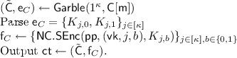
\(\mathsf {Dec} (\mathsf {sk} = (\mathsf {k},\sigma ),\mathsf {ct} = (\tilde{\mathsf {C}},\mathsf {f}_C))\):


Note in particular that the secret key \(\mathsf {sk} \) does not include the signing key \(\mathsf {sgk}\).
6.1 Correctness
We will first show that the scheme \(\mathsf {PKE} \) is correct. Let therefore \((\mathsf {pk},\mathsf {sk}) \leftarrow \mathsf {PKE}.\mathsf {KeyGen} (1^\kappa )\) and \(\mathsf {ct} \leftarrow \mathsf {PKE}.\mathsf {Enc} (\mathsf {pk},\mathsf {m})\). By the correctness of the OTSE-scheme \(\mathsf {NC}\) it holds that \(\tilde{\mathsf {k}} = \{ K_{j,\mathsf {k}_j} \}\). Thus, by the correctness of the garbling scheme it holds that \(\mathsf {ct} ' = \tilde{\mathsf {C}}[\mathsf {m} ](\mathsf {k}) = \mathsf {SKE}.\mathsf {Enc} (\mathsf {k},\mathsf {m})\). Finally, by the correctness of \(\mathsf {SKE}\) it holds that \(\mathsf {SKE}.\mathsf {Dec} (\mathsf {k},\mathsf {ct} ') = \mathsf {m} \).
6.2 Security
We will now show that \(\mathsf {PKE} \) is \(\mathsf {KDM}^{\mathsf {CPA}}\)-secure.
Theorem 7
Assume that \(\mathsf {NC}\) is an \(\mathsf {IND}^{\mathsf {OTSIG}}\)-secure OTSE-scheme and \((\mathsf {Garble},\mathsf {Eval})\) is a secure garbling scheme. Let \(\mathcal {F}\) be a class of KDM-functions and assume that the function \(g_{\mathsf {pp},\mathsf {sgk}}: x \mapsto (x,\mathsf {NC}.\mathsf {SSign} (\mathsf {pp},\mathsf {sgk}, x))\) is in a class \(\mathcal {G}\) (e.g. affine functions). Assume that \(\mathsf {SKE}\) is a \(\mathsf {KDM}^{\mathsf {CPA}}\)-secure secret-key encryption scheme for the class \(\mathcal {F} \circ \mathcal {G}\). Then \(\mathsf {PKE} \) is a \(\mathsf {KDM}^{\mathsf {CPA}}\)-secure public key encryption scheme for the class \(\mathcal {F}\).
Note that if both \(\mathcal {F}\) and \(\mathcal {G}\) are the class of affine functions, e.g. over \(\mathbb {F}_2\), then \(\mathcal {F} \circ \mathcal {G}\) is again the class of affine functions (over \(\mathbb {F}_2\)). Thus, every function in \(\mathcal {F} \circ \mathcal {G}\) can also be implemented as an affine function, i.e. by a matrix-vector product followed by an addition.
Proof
Let \(\mathcal {A} \) be a PPT-adversary against the \(\mathsf {KDM}^{\mathsf {CPA}}\)-security of \(\mathsf {PKE}\). Consider the following hybrids, in which we will change the way the KDM-oracle is implemented. For sake of readability, we only provide 3 hybrids, where in actuality each hybrid consists of q sub-hybrids, where q is the number of KDM-queries of \(\mathcal {A} \).
Hybrid \(\mathcal {H} _1\) : This hybrid is identical to the \(\mathsf {KDM}^{\mathsf {CPA}}\)-experiment.
Hybrid \(\mathcal {H} _2\) : This hybrid is identical to \(\mathcal {H} _1\), except that \(\mathsf {f}_C \) is computed by \(\mathsf {f}_C \leftarrow \{ \mathsf {NC}.\mathsf {SEnc} (\mathsf {pp},(\mathsf {vk},j,b),K_{j,\mathsf {k}_j}) \}_{j \in [\kappa ], b \in \{0,1\}}\), i.e. for each \(j \in [\kappa ]\) we encrypt \(K_{j,\mathsf {k}_j}\) twice, instead of \(K_{j,0}\) and \(K_{j,1}\). By the \(\mathsf {IND}^{\mathsf {OTSIG}}\)-security of \(\mathsf {NC}\) the hybrids \(\mathcal {H} _1\) and \(\mathcal {H} _2\) are computationally indistinguishable.
Hybrid \(\mathcal {H} _3\) : This hybrid is identical to \(\mathcal {H} _2\), except that we compute \(\tilde{\mathsf {C}}\) and \(\mathsf {f}_C \) by \((\tilde{\mathsf {C}},\tilde{\mathsf {k}}) \leftarrow \mathsf {GCSim} (\mathsf {C},\mathsf {C} [\mathsf {m} ](\mathsf {k}))\). Computational indistinguishability between \(\mathcal {H} _2\) and \(\mathcal {H} _3\) follows by the security of the garbling scheme \((\mathsf {Garble},\mathsf {Eval})\). Notice that it holds that \(\mathsf {C} [\mathsf {m} ^*](\mathsf {k}) = \mathsf {SKE}.\mathsf {Enc} (\mathsf {k},\mathsf {m} ^*)\).
We will now show that the advantage of \(\mathcal {A} \) is negligible in \(\mathcal {H} _3\), due to the \(\mathsf {KDM}^{\mathsf {CPA}}\)-security of \(\mathsf {SKE}\). We will provide a reduction \(\mathsf {R} \) such that \(\mathsf {R} ^\mathcal {A} \) has the same advantage against the \(\mathsf {KDM}^{\mathsf {CPA}}\)-security of \(\mathsf {SKE}\) as \(\mathcal {A} \)’s advantage against \(\mathcal {H} _3\).
Before we provide the reduction \(\mathsf {R} \), notice that \(\mathsf {R} \) does not have access to its own challenge secret key \(\mathsf {k}\), which is part of the secret key \(\mathsf {sk} = (\mathsf {k},\sigma )\) of the resulting PKE. Also, since \(\sigma \) is a signature on k, \(\mathsf {R} \) does not know the value of \(\sigma \) either. Thus, \(\mathsf {R} \) cannot on its own simulate encryptions of messages that depend on \((\mathsf {k}, \sigma )\). We overcome this problem by using the KDM-oracle provided to \(\mathsf {R} \) which effectively allows \(\mathsf {R} \) to obtain encryptions of key-dependent messages \(\mathsf {sk} = (\mathsf {k},\sigma )\). Details follow.
The reduction \(\mathsf {R} \) first samples \(\mathsf {pp}\leftarrow \mathsf {NC}.\mathsf {SSetup} (1^\kappa ,\kappa )\) and \((\mathsf {vk},\mathsf {sgk}) \leftarrow \mathsf {NC}.\mathsf {SGen} (\mathsf {pp})\) and invokes \(\mathcal {A} \) on \(\mathsf {pk} = (\mathsf {pp},\mathsf {vk})\). Then \(\mathsf {R} \) simulates \(\mathcal {H} _3\) for \(\mathcal {A} \) with the following differences. Whenever \(\mathcal {A} \) queries the KDM-oracle with a function \(f \in \mathcal {F}\), the reduction \(\mathsf {R} \) programs a new function \(f' \in \mathcal {F} \circ \mathcal {G}\) which is defined by
We assume for simplicity that the signing procedure \(\mathsf {NC}.\mathsf {SSign} \) is deterministic, if not we require that the same randomness r is used for \(\mathsf {NC}.\mathsf {SSign} \) at each KDM-queryFootnote 3.
We claim that \(\mathsf {R} \) simulates \(\mathcal {H} _3\) perfectly from the view of \(\mathcal {A} \). If the challenge-bit in \(\mathsf {R} \)’s \(\mathsf {KDM}^{\mathsf {CPA}}\)-experiment is 0, then the outputs of \(\mathcal {A} \)’s KDM-oracle on input f are encryptions of \(f'(\mathsf {k}) = f(\mathsf {sk})\), and therefore, from the view of \(\mathcal {A} \) the challenge-bit in \(\mathcal {H} _3\) is also 0. On the other hand, if the challenge-bit in \(\mathsf {R} \)’s \(\mathsf {KDM}^{\mathsf {CPA}}\)-experiment is 1, then the outputs of \(\mathcal {A} \)’s KDM-oracle on input f are encryptions of \(0^\ell \), and therefore, from \(\mathcal {A} \)’s view the challenge-bit in \(\mathcal {H} _3\) is 1. We conclude that the advantage of \(\mathsf {R} ^\mathcal {A} \) is identical to the advantage of \(\mathcal {A} \) against \(\mathcal {H} _3\). It follows from the \(\mathsf {KDM}^{\mathsf {CPA}}\)-security of \(\mathsf {SKE}\) that the latter is negligible, which concludes the proof. \(\square \)
Notes
- 1.
We also need to hardcode the randomness for \(\mathsf {NC}.\mathsf {SEnc} \) into \(\mathsf {C} \), but for ease of notation we omit this parameter.
- 2.
We also need to hardcode the randomness for \(\mathsf {SKE}.\mathsf {Enc} \) into \(\mathsf {C} \), but for ease of notation we omit this parameter.
- 3.
This does not pose a problem as we always sign the same message \(\mathsf {k}\) at each KDM-query.
References
Agrawal, S., Boneh, D., Boyen, X.: Efficient lattice (H)IBE in the standard model. In: Gilbert, H. (ed.) EUROCRYPT 2010. LNCS, vol. 6110, pp. 553–572. Springer, Heidelberg (2010). https://doi.org/10.1007/978-3-642-13190-5_28
Arora, S., Babai, L., Stern, J., Sweedyk, Z.: The hardness of approximate optimia in lattices, codes, and systems of linear equations. In: 34th FOCS, Palo Alto, California, 3–5 November 1993, pp. 724–733. IEEE Computer Society Press (1993)
Applebaum, B., Cash, D., Peikert, C., Sahai, A.: Fast cryptographic primitives and circular-secure encryption based on hard learning problems. In: Halevi, S. (ed.) CRYPTO 2009. LNCS, vol. 5677, pp. 595–618. Springer, Heidelberg (2009). https://doi.org/10.1007/978-3-642-03356-8_35
Ajtai, M.: The shortest vector problem in L2 is NP-hard for randomized reductions (extended abstract). In: 30th ACM STOC, Dallas, TX, USA, 23–26 May 1998, pp. 10–19. ACM Press (1998)
Alekhnovich, M.: More on average case vs approximation complexity. In: 44th FOCS, Cambridge, MA, USA, 11–14 October 2003, pp. 298–307. IEEE Computer Society Press (2003)
Alperin-Sheriff, J., Peikert, C.: Circular and KDM security for identity-based encryption. In: Fischlin, M., Buchmann, J., Manulis, M. (eds.) PKC 2012. LNCS, vol. 7293, pp. 334–352. Springer, Heidelberg (2012). https://doi.org/10.1007/978-3-642-30057-8_20
Applebaum, B.: Key-dependent message security: generic amplification and completeness. J. Cryptol. 27(3), 429–451 (2014)
Boneh, D., Boyen, X.: Secure identity based encryption without random oracles. In: Franklin, M. (ed.) CRYPTO 2004. LNCS, vol. 3152, pp. 443–459. Springer, Heidelberg (2004). https://doi.org/10.1007/978-3-540-28628-8_27
Boneh, D., Franklin, M.K.: Identity-based encryption from the weil pairing. In: Kilian, J. (ed.) CRYPTO 2001. LNCS, vol. 2139, pp. 213–229. Springer, Heidelberg (2001). https://doi.org/10.1007/3-540-44647-8_13
Blum, A., Furst, M.L., Kearns, M.J., Lipton, R.J.: Cryptographic primitives based on hard learning problems. In: Stinson, D.R. (ed.) CRYPTO 1993. LNCS, vol. 773, pp. 278–291. Springer, Heidelberg (1994). https://doi.org/10.1007/3-540-48329-2_24
Brakerski, Z., Goldwasser, S.: Circular and leakage resilient public-key encryption under subgroup indistinguishability - (or: Quadratic residuosity strikes back). In: Rabin, T. (ed.) CRYPTO 2010. LNCS, vol. 6223, pp. 1–20. Springer, Heidelberg (2010). https://doi.org/10.1007/978-3-642-14623-7_1
Boneh, D., Gentry, C., Hamburg, M.: Space-efficient identity based encryption without pairings. In: 48th FOCS, Providence, RI, USA, 20–23 October 2007, pp. 647–657. IEEE Computer Society Press (2007)
Barak, B., Haitner, I., Hofheinz, D., Ishai, Y.: Bounded key-dependent message security. In: Gilbert, H. (ed.) EUROCRYPT 2010. LNCS, vol. 6110, pp. 423–444. Springer, Heidelberg (2010). https://doi.org/10.1007/978-3-642-13190-5_22
Boneh, D., Halevi, S., Hamburg, M., Ostrovsky, R.: Circular-secure encryption from decision Diffie-Hellman. In: Wagner, D. (ed.) CRYPTO 2008. LNCS, vol. 5157, pp. 108–125. Springer, Heidelberg (2008). https://doi.org/10.1007/978-3-540-85174-5_7
Bellare, M., Hoang, V.T., Rogaway, P.: Foundations of garbled circuits. In: Yu, T., Danezis, G., Gligor, V.D. (eds.) ACM CCS 2012, Raleigh, NC, USA, 16–18 October 2012, pp. 784–796. ACM Press (2012)
Brakerski, Z., Lombardi, A., Segev, G., Vaikuntanathan, V.: Anonymous IBE, leakage resilience and circular security from new assumptions. Cryptology ePrint Archive, Report 2017/967 (2017). http://eprint.iacr.org/2017/967
Cho, C., Döttling, N., Garg, S., Gupta, D., Miao, P., Polychroniadou, A.: Laconic oblivious transfer and its applications. In: Katz, J., Shacham, H. (eds.) CRYPTO 2017. LNCS, vol. 10402, pp. 33–65. Springer, Cham (2017). https://doi.org/10.1007/978-3-319-63715-0_2
Canetti, R., Halevi, S., Katz, J.: Chosen-ciphertext security from identity-based encryption. In: Cachin, C., Camenisch, J.L. (eds.) EUROCRYPT 2004. LNCS, vol. 3027, pp. 207–222. Springer, Heidelberg (2004). https://doi.org/10.1007/978-3-540-24676-3_13
Cash, D., Hofheinz, D., Kiltz, E., Peikert, C.: Bonsai trees, or how to delegate a lattice basis. In: Gilbert, H. (ed.) EUROCRYPT 2010. LNCS, vol. 6110, pp. 523–552. Springer, Heidelberg (2010). https://doi.org/10.1007/978-3-642-13190-5_27
Cash, D., Hofheinz, D., Kiltz, E., Peikert, C.: Bonsai trees, or how to delegate a lattice basis. J. Cryptol. 25(4), 601–639 (2012)
Cocks, C.: An identity based encryption scheme based on quadratic residues. In: Honary, B. (ed.) Cryptography and Coding 2001. LNCS, vol. 2260, pp. 360–363. Springer, Heidelberg (2001). https://doi.org/10.1007/3-540-45325-3_32
Döttling, N., Garg, S.: From selective IBE to full IBE and selective HIBE. In: Kalai, Y., Reyzin, L. (eds.) TCC 2017. LNCS, vol. 10677, pp. 372–408. Springer, Cham (2017). https://doi.org/10.1007/978-3-319-70500-2_13
Döttling, N., Garg, S.: Identity-based encryption from the Diffie-Hellman assumption. In: Katz, J., Shacham, H. (eds.) CRYPTO 2017. LNCS, vol. 10401, pp. 537–569. Springer, Cham (2017). https://doi.org/10.1007/978-3-319-63688-7_18
Döttling, N., Müller-Quade, J., Nascimento, A.C.A.: IND-CCA secure cryptography based on a variant of the LPN problem. In: Wang, X., Sako, K. (eds.) ASIACRYPT 2012. LNCS, vol. 7658, pp. 485–503. Springer, Heidelberg (2012). https://doi.org/10.1007/978-3-642-34961-4_30
Döttling, N.: Low noise LPN: KDM secure public key encryption and sample amplification. In: Katz, J. (ed.) PKC 2015. LNCS, vol. 9020, pp. 604–626. Springer, Heidelberg (2015). https://doi.org/10.1007/978-3-662-46447-2_27
Gentry, C., Peikert, C., Vaikuntanathan, V.: Trapdoors for hard lattices and new cryptographic constructions. In: Ladner, R.E., Dwork, C. (eds.) 40th ACM STOC, Victoria, British Columbia, Canada, 17–20 May 2008, pp. 197–206. ACM Press (2008)
Guruswami, V., Rudra, A.: Soft decoding, dual BCH codes, and better list-decodable \(\varepsilon \)-biased codes. IEEE Trans. Information Theory 57(2), 705–717 (2011)
Håstad, J., Impagliazzo, R., Levin, L.A., Luby, M.: A pseudorandom generator from any one-way function. SIAM J. Comput. 28(4), 1364–1396 (1999)
Haviv, I., Regev, O.: Tensor-based hardness of the shortest vector problem to within almost polynomial factors. In: Johnson, D.S., Feige, U. (eds.) 39th ACM STOC, San Diego, CA, USA, 11–13 June 2007, pp. 469–477. ACM Press (2007)
Khot, S.: Hardness of approximating the shortest vector problem in lattices. In: 45th FOCS, Rome, Italy, 17–19 October 2004, pp. 126–135. IEEE Computer Society Press (2004)
Kiltz, E., Masny, D., Pietrzak, K.: Simple chosen-ciphertext security from low-noise LPN. In: Krawczyk, H. (ed.) PKC 2014. LNCS, vol. 8383, pp. 1–18. Springer, Heidelberg (2014). https://doi.org/10.1007/978-3-642-54631-0_1
Kitagawa, F., Tanaka, K.: Key dependent message security and receiver selective opening security for identity-based encryption. Cryptology ePrint Archive, Report 2017/987 (2017). http://eprint.iacr.org/2017/987
Lenstra, A.K., Lenstra, H.W., Lovász, L.: Factoring polynomials with rational coefficients. Math. Ann. 261(4), 515–534 (1982)
Lindell, Y., Pinkas, B.: A proof of security of Yao’s protocol for two-party computation. J. Cryptol. 22(2), 161–188 (2009)
Lewko, A.B., Waters, B.: New techniques for dual system encryption and fully secure HIBE with short ciphertexts. In: Micciancio, D. (ed.) TCC 2010. LNCS, vol. 5978, pp. 455–479. Springer, Heidelberg (2010). https://doi.org/10.1007/978-3-642-11799-2_27
Lyubashevsky, V., Wichs, D.: Simple lattice trapdoor sampling from a broad class of distributions. In: Katz, J. (ed.) PKC 2015. LNCS, vol. 9020, pp. 716–730. Springer, Heidelberg (2015). https://doi.org/10.1007/978-3-662-46447-2_32
Micciancio, D.: The shortest vector in a lattice is hard to approximate to within some constant. In: 39th FOCS, Palo Alto, CA, USA, 8–11 November 1998, pp. 92–98. IEEE Computer Society Press (1998)
Micciancio, D., Peikert, C.: Trapdoors for lattices: simpler, tighter, faster, smaller. In: Pointcheval, D., Johansson, T. (eds.) EUROCRYPT 2012. LNCS, vol. 7237, pp. 700–718. Springer, Heidelberg (2012). https://doi.org/10.1007/978-3-642-29011-4_41
Micciancio, D., Regev, O.: Worst-case to average-case reductions based on Gaussian measures. In: 45th FOCS, Rome, Italy, 17–19 October 2004, pp. 372–381. IEEE Computer Society Press (2004)
Regev, O.: On lattices, learning with errors, random linear codes, and cryptography. In: Gabow, H.N., Fagin, R. (eds.) 37th ACM STOC, Baltimore, MA, USA, 22–24 May 2005, pp. 84–93. ACM Press (2005)
Shamir, A.: Identity-based cryptosystems and signature schemes. In: Blakley, G.R., Chaum, D. (eds.) CRYPTO 1984. LNCS, vol. 196, pp. 47–53. Springer, Heidelberg (1985). https://doi.org/10.1007/3-540-39568-7_5
Waters, B.R.: Efficient identity-based encryption without random oracles. In: Cramer, R. (ed.) EUROCRYPT 2005. LNCS, vol. 3494, pp. 114–127. Springer, Heidelberg (2005). https://doi.org/10.1007/11426639_7
Waters, B.: Dual system encryption: realizing fully secure IBE and HIBE under simple assumptions. In: Halevi, S. (ed.) CRYPTO 2009. LNCS, vol. 5677, pp. 619–636. Springer, Heidelberg (2009). https://doi.org/10.1007/978-3-642-03356-8_36
Yao, A.C.-C.: Protocols for secure computations (extended abstract). In: 23rd FOCS, Chicago, Illinois, 3–5 November 1982, pp. 160–164. IEEE Computer Society Press (1982)
Yu, Y., Zhang, J.: Cryptography with auxiliary input and trapdoor from constant-noise LPN. In: Robshaw, M., Katz, J. (eds.) CRYPTO 2016. LNCS, vol. 9814, pp. 214–243. Springer, Heidelberg (2016). https://doi.org/10.1007/978-3-662-53018-4_9
Author information
Authors and Affiliations
Corresponding authors
Editor information
Editors and Affiliations
Rights and permissions
Copyright information
© 2018 International Association for Cryptologic Research
About this paper

Cite this paper
Döttling, N., Garg, S., Hajiabadi, M., Masny, D. (2018). New Constructions of Identity-Based and Key-Dependent Message Secure Encryption Schemes. In: Abdalla, M., Dahab, R. (eds) Public-Key Cryptography – PKC 2018. PKC 2018. Lecture Notes in Computer Science(), vol 10769. Springer, Cham. https://doi.org/10.1007/978-3-319-76578-5_1
Download citation
DOI: https://doi.org/10.1007/978-3-319-76578-5_1
Published:
Publisher Name: Springer, Cham
Print ISBN: 978-3-319-76577-8
Online ISBN: 978-3-319-76578-5
eBook Packages: Computer ScienceComputer Science (R0)
