
Abstract
The following chapter considers the main principles of valuation, from a company valuation perspective but also from a valuation perspective on assets and projects.
Access this chapter
Tax calculation will be finalised at checkout
Purchases are for personal use only
Notes
- 1.
See Eayrs et al. (2011, p 281–283).
- 2.
In practice, companies have more freedom for the framework and setup of the valuation they perform compared to the framework which IFRS is setting for valuations. Whereas IFRS requires to follow the market (e.g. capital structure for the calculation of the cost of capital is derived from the peer group), companies can also derive the cost of capital from the company-specific data and target (e.g. target capital structure of the company for the calculation of the cost of capital of this company). Furthermore, IFRS also sets guidelines on the valuation framework as such (e.g. IFRS 9 on the valuation of financial instruments).
- 3.
Generally, assumptions can be split into (a) general assumptions and general financial/economic assumptions and (b) business-specific assumptions (e.g. optimization assumptions and results of assets as calculated, e.g. by Linear Programming. For further literature see Denardo (2011), or Dorfmanet al. (1958).
- 4.
It might be the case that the application of a Terminal Value (in form of a perpetuity as well as in form of a multiple) is not appropriate and that, e.g. due to contractual or business planning reasons, the detailed period comprises much more than 3–5 years, for example, up to 40 or 50 years or longer.
- 5.
In practice, 360 days are also sometimes used for the simulation of an entire business year.
- 6.
An element specific to the energy industry is the concept of current cost of supply (CCS) which aims to measure the true performance of business as independent from potential improvements or declines caused by to the volatility of prices. To use a refinery as an example, the CCS result will be measured by eliminating any price changes such as the increased price of crude oil in the respective reporting period, thereby eliminating any ‘windfall profits’ in order to show a fair view of the operative performance. The overall performance, which is measured in the reported result, will include the CCS effects. The differentiation between the CCS result and the reported result is a potential source of data mismatch, which is the basis for the cash flow derivation.
- 7.
Technically, all positions of the cash flow can be derived from the balance sheet.
- 8.
For example, valuations can be used for the determination of a potential purchase or sales prices of a company, or of parts of a company, and also for others purposes including the assessment of the sustainability of a company’s assets or participations (impairment testing), the valuation of the shares in a company, etc. Valuations for IFRS purposes follow partially different rules (e.g. the discount rate will be different for a valuation for IFRS purposes from the discount rate for a valuation for mergers and acquisition purposes).
- 9.
In this instance, Free Cash Flows mean ‘Free Cash Flows to Firm (FCFF)’ (as opposed to ‘Free Cash Flows to Equity (FCFE)’.
- 10.
The Free Cash Flow concept, as described in this chapter, does not take into account the impact from financing. The impact from financing is already reflected in the cost of capital (i.e. the discount rate). In accounting, the Free Cash Flow takes into account the impacts of financing on the profit and loss statement (i.e. impact on the financial result).
- 11.
In contrast to the Free Cash Flow approach, the Total Cash Flow (‘TCF’) approach simulates the taxes which are calculated as though a finance result were included in the calculation. In this numeric example, the TCF will use the taxes of −16.25 mn EUR. As the TCF depicts the tax shield in the cash flows, the discount rate of the TCF approach does not contain any tax shield. The Free Cash Flow depicted to be used for valuation purpose might not be identical to the Free Cash Flow which is used, in practice, for Annual Reports or for performance management as the Free Cash Flow for valuation purposes does not include any impact from financing.
- 12.
Provision movements with a financing character shall not be shown in the operative result (e.g. provisions for so-called social capital, including retirement etc.). Eventually, the operative results have to be adjusted to accommodate such provisions, which are deducted from the Entity value of the company when the Equity value is derived. The movements of provisions should be neutralized by the position ‘+/− Posting/release of ‘operative’ provisions’ for the derivation of the Free Cash Flow.
- 13.
Net Working Capital (NWC) = Current Assets − Current Liabilities + Inventories. The inventory management of a refinery will serve as an example for a net working capital increase: In order to be flexible in production (short-term decision between maximising the fuel production or the petrochemical production in a refinery), the management of a refinery builds up a larger inventory of crude oil in the refinery’s tanks. This increased level of inventory has to be paid to the crude oil supplier, and the monetization of the finished products of the refinery will take place at a later point in time. The increase of the inventory leads to a cash outflow. The decrease of the inventory when the products are sold leads to a cash inflow.
Another example is a gas filling station: Generally, a filling station does not have many receivables as the customers pay immediately at the fuel pump. The filling station will have an inventory (e.g. tanks for gasoline and diesel) and will incur some payables as the deliveries of substances such as gasoline and diesel are not normally paid immediately, but rather some days or weeks later. Overall, a filling station shows in general a negative net working capital. Remark: the valuation examples in this chapter will use the term ‘Working Capital ’ instead of ‘Net Working Capital’.
- 14.
This valuation method is also called the ‘sum-of-the parts method’. It is used especially for transparency and in order to benchmark the segments of the business (i.e. the separate parts of the company). The difficulty with this method is setting up separate financial statements, especially the elimination of intercompany relations and the proper allocation of general, corporate expenses. Please refer to Sects. 4.6.1.1 ‘NPV in interaction with other KPIs’ and 4.6.1.2 for an introduction on the basis for sum-of-the-parts valuations.
- 15.
A tolling agreement is an agreement where the so-called toller agrees with the owner of raw material(s) to process these raw material(s) for a certain fee, which is known as the ‘toll’. The toller converts the raw material(s) into a product which remains the property of the owner of the raw material(s) provided. A practical example could be a refinery, where the owner of the crude oil provides the crude to the refinery company. The refinery produces gasoline and diesel out of the provided crude oil and receives a fee from the provider of the crude oil.
- 16.
A good check in practice is if the assumptions are described properly (data sources, data providers, etc.) and in detail (are they the appropriate assumptions in light of past and future market developments? Are legal, technical and commercial developments covered by these assumptions?).
- 17.
The Terminal Value has to be discounted in order to be comparable with the Entity Value as the Entity Value represents the discounted Free Cash Flows of the future (under the assumption that there is no sale of assets, which are no longer needed for the company’s operation, foreseen).
- 18.
This depends on various factors such as length of the single years’ period, cash flow profile, discount rate, etc. A general statement in this context is hardly possible. The percentages stated here should only serve as a very rough indication. Reference is made to Koller et al. (2015, p 271f), where the share of discounted Terminal Value is stated in a range from approximately 80%–85%.
- 19.
This formula is derived from the Gordon Growth Model.
- 20.
In case the growth rate is greater than the interest rate, the Terminal Value will become negative. In practice, this should not take place.
- 21.
This assumption is only correct if zero growth is assumed for the Terminal Value period. More details are provided in the section ‘Invested Capital’ in this subchapter.
- 22.
This formula is identical in result as the previous one if the growth rate is set to zero.
- 23.
If a company has no fixed costs, the ‘degree of operating leverage’ is one.
- 24.
In practice, IFRS provides guidance by five minimum requirements for the profit and loss statement (IAS 1.82). Key performance indicators can be defined based on operational and financial requirements of the respective company and based on the management and steering framework.
- 25.
In practice, IFRS provides guidance by five minimum requirements for the profit and loss statement (IAS 1.81). Key performance indicators can be defined based on operational and financial requirements of the respective company and based on the management and steering framework.
- 26.
The following issues should be considered with regard to the EBIT: first, the difference between the so-called ‘clean’ and ‘reported’ result. The EBIT may contain extraordinary results, which are not part of the ordinary course of business. For example, if an energy company sells at one of its filling stations fuels, it is the normal, ordinary business of an energy company. If the energy company decides to sell the land plot of the filling station, it will also be recorded in the EBIT, even though it is not a normal business transaction of an energy company. The selling of the land is an extraordinary transaction for an energy company as it is not a real estate company. The selling of the land is therefore a special item. Such special items will be deducted (or also added depending on the respective case) from the EBIT in order to calculate a ‘Clean EBIT,’ which contains no special items and is therefore not affected by any extraordinary results. The Clean EBIT provides a better understanding of the true operational performance. The EBIT containing the special items (such as the sale of the land in our example) is called a ‘Reported EBIT.’ The second special characteristic of an EBIT, which is especially the case in the energy industry, is the so-called CSS EBIT. ‘CCS’ stands for ‘current cost of supply’. The current cost of supply concept applies to the time difference between the purchase of a commodity and the selling of it or of the end-product which has been produced out of the commodity in the meantime. For example, there is a current cost of supply-effect for fuel. If crude oil is purchased at a certain price, there might be some price volatility between the purchase of the crude oil and the sale of the fuel, which is produced using the crude oil. If the crude oil price is at 50 USD per barrel at the point of time of purchase but has increased to 60 USD per barrel by the time the produced fuel reaches the filling station, the crude oil price and the selling price of the fuel will be significantly higher than previous fuel price. The current cost of supply-concept breaks this balance by assuming that the purchase of the crude oil has been undertaken at the same crude oil price as was valid at the time of sale of the fuel (in this example here 60 USD per barrel) and therefore eliminates the increase in the price of crude oil and its effect on the price of fuel. The assumption is that the input commodity for the fuel, the crude oil, has been purchased at the currently prevailing price. The concept is therefore called ‘current cost of supply.’ The appliance of the CCS result logic can be demonstrated in the measurement of the actual operating performance of a refinery. If adjusted by the current cost of supply, the Clean EBIT is called ‘Clean CCS EBIT’. This Clean CCS EBIT helps to compare the operational business performance of previous years (especially if there have been large price volatilities between the years) and to compare the valuation target performance of the company against its peers. A Clean CCS EBIT is a widely used concept in the energy industry. While the Clean CCS EBIT is used for comparisons, the reported EBIT must be used the valuation. If a Clean CCS EBIT is used for a valuation, the special items and the current cost of supply-effects have to be added back in so that the starting base line for the valuation is ultimately the reported EBIT.
- 27.
There are also cases that the Invested Capital is defined as the total balance sheet sum. The definition depends on a case-by-case basis.
- 28.
This assumption may lead to the ‘aggressive’ growth formula for the Terminal Value. NOPLAT instead of Free Cash Flow is used, and then NOPLAT divided by (i−g) is the formula for the Terminal Value calculation.
- 29.
Reference is made to Sect. 5.10.
- 30.
From a technical standpoint, inflation covers a broad range of definitions, and there are various inflation rates available. Various consumer price indices or—in a narrower, more detailed range—certain producer price indices are generally available. The selecting of a rate to take as growth rate and whether this rate is represented best by an inflation rate (and then by which inflation rate) changes on a case-by-case basis.
- 31.
For the calculation or the Return on Equity (‘ROE‘):
$$ \mathrm{RO}{\mathrm{E}}_t=\frac{\mathrm{NOPLA}{\mathrm{T}}_t-\mathrm{Financial}\ \mathrm{Resul}{\mathrm{t}}_t}{\mathrm{Invested}\ \mathrm{Capita}{\mathrm{l}}_{t-1}-\mathrm{Net}\ \mathrm{Deb}{\mathrm{t}}_{t-1}}=\frac{\mathrm{Net}\ \mathrm{Incom}{\mathrm{e}}_t}{\mathrm{E}\mathrm{quit}{\mathrm{y}}_{t-1}} $$ - 32.
This concept is similar to the Economic Value Added concept; please see Sect. 2.4.
- 33.
Being it Free Cash Flow, Equity Cash Flow or other kinds of cash flow.
- 34.
This summary is only valid for Terminal Values which are derived by a perpetuity. In cases which do not justify the appliance of a perpetuity, the interplay of single years’ planning and Terminal Value as described here is not applicable. Terminal Values in form of a multiple are recommended for plausibility purposes.
- 35.
This is an exception to the general rule that the discount factor for the discounting of the Terminal Value has to be identical with the discount factor of the last single planning year. This is because the years shown here are not single planning years of the detailed planning period (‘Phase 1’) but years of the Terminal Value period as such.
- 36.
This is one way to simulate a convergence. There are other ways to simulate a convergence of ROIC towards cost of capital during the Terminal Value period; please see the calculation approaches described on the next pages. Another way to derive a valuation result, which is similar to one derived by convergence formula, is to cut of the Terminal Value period manually, e.g. after the first 30 years of the Terminal Value period.
- 37.
This formula follows the so-called ‘Gordon Growth Model’. The original Gordon Growth Model refers to valuation on basis of dividends (dividend discount model).
- 38.
Reference is made to Koller et al. (2015).
- 39.
- 40.
For specifics on Upstream, please refer to Kasriel and Wood (2013) and Wright and Gallun (2008).
If the valuation target has a finite lifetime (e.g. finite resources of hydrocarbons in a reservoir), a Terminal Value should not be used. Instead the valuation should be carried out on a single years’ planning and (eventually) include decommissioning of the valuation target.
Examples could include the upstream segment with valuation period consisting of purely single planning years (which might even cover the entire period of a production agreement of 30 years or longer) and potentially incorporating the cash flows related to decommissioning (cash-in from liquidation, cash-out from closure of activities, decommissioning the production area, etc.) or other assets or companies which cannot take the assumption of eternal continuation (e.g. assets/companies which are exposed to technical progress and updates on a constant basis might assume that the technics set a limit to their economic usage and existence or value added).
Valuations in the upstream segment follow the same general principles and methods as valuations in other parts of the energy industry.
There are two main issues which deserve more attention in cases of valuations in the upstream segment than in other value chain elements:
-
1.
Upstream might face comparatively more and severer risks than other segments of the value chain. The proper planning, potential mitigation (if possible) and reflection of risks in the cash flow planning are the key factors for the upstream valuations and of comparatively even higher importance than in other value chain elements.
-
2.
The second issue, which is connected to the crucial importance of risk reflection in the cash flows, is the fact that taxes might take a significant place in the valuation. Taxes might range at high levels and might take a major portion of the cash flows, profitability and valuation result. Taxes in the upstream segment of hydrocarbons can be classified in three broad categories:
-
(a)
Concession: Under a concession, an oil and gas company is granted exclusive rights to the exploration and production of the so-called concession area. The company owns the production of hydrocarbons. Generally, the company pays so-called royalties and corporate income tax. There might also be additional (fiscal) payments stipulated such as rentals, resource taxes, special petroleum or windfall profit taxes, export duties, etc. It might also be the case that—in cases where international energy companies are active in the respective host country—the law of the host country requires a state participation or participation of a company of the host country.
-
(b)
Production sharing contract (‘PSC’)/production sharing agreement (‘PSA’): Under a PSC/PSA, an international energy company concludes a contract with a national energy company or a host government. As a general description, the international energy company is responsible for the financing and the exploration and production and—in counterturn—receives a certain portion of the hydrocarbons produced ( ‘cost oil/gas’) and the profits ( ‘profit oil/gas’). There might be cases in which other payments such as royalties, corporate income tax or windfall profit taxes must also be made to the host government. Royalties are charged on the basis of gross revenues, which might discourage new investments into drilling and production. In incremental economic situations, royalties may work in the opposite direction: if the gross revenues are high and the royalties percentage is not excessively high, the international energy company might be encouraged to continue the operations and not to abandon this marginal field. One tool to counter-steer any discouraging effects of royalties is to use so-called sliding scale royalties. For example, the royalty rate could be 10% for a production range from 0 up to 10,000 bbl/day, 15% for a production range of 10,001 bbl/day–15,000 bbl/day and 20% for a production range above 15,001 bbl/day.
-
(c)
Service contracts: Generally, the international energy company finances the projects and explores and produces the hydrocarbons. In counterturn, it receives a fee in cash or in kind.
-
(a)
Another element which might be different in the upstream segment versus other segments or industries is the deprecation method. In the upstream segment, it might be the case that depreciation methods other than a linear deprecation scheme are used (for accounting and/or tax purposes as well). An example of a widely used depreciation scheme is the so-called unit-of-production method. This method is not a linear method but uses a different rate of depreciation for each period. The respective rate is derived by dividing the production of the period by the estimated reserves at beginning of the period. The depreciation (unit-of-production) is calculated by multiplying the rate of the respective period by the book value of the asset at the beginning of the period. The effect of the unit-of-production depreciation is that the depreciation follows the production level (which must not be identical with the value of the production).
Terminal Value for Downstream
For the downstream segment, the Terminal Value can be used on a case-by-case basis.
The usage of a Terminal Value is dependent on the business model and the type of asset of the respective valuation.
For example, it is generally not the case that a valuation of a gas-fired power plant will consider a Terminal Value in form of a perpetuity as the technological development will progress continuously and the power plant will fall out of the market as new, technically more developed, and therefore more profitable power plants will enter the market.
There are other valuation targets in which it is suitable to consider a Terminal Value; for example, a retail network might involve a Terminal Value.
As the decision to apply a Terminal Value has to be taken on a case-by-case basis, the only general rule on whether or not and how to apply a Terminal Value in form of a perpetuity is that it has to be considered as to whether there is a long-term persistence and development to be planned or not (i.e. if finite factors limit the long-term persistence of the business model of the valuation target).
-
1.
- 41.
From this section onwards, the data of the integrated planning of the energy company is used.
- 42.
Bludgeon Approach, r E = rfr + MRP × β + CRP; used when all entities are equally weighted with the country risk
Beta Approach, r E = rfr + (MRP + CRP) × β; used when the country risk adapts proportionally to the market risk
Lambda Approach, r E = rfr + (MRP × β MRP) + (CRP × β CRP); used when there is no relationship between country risk and market risk
Lüdenbach and Hoffmann (2010).
- 43.
Disregarding potential differences due to the timing of dividend payout and potential taxation applicable to the dividend payments.
- 44.
The depictions of the figure assume that there are no ‘excess cash’ and no assets which are not needed for the continuation of operations.
- 45.
In the detailed planning of the single years‘ planning period (‘Phase 1‘), the development of debt (financial liabilities) is planned in a detailed way (i.e. deterministic planning of the debt). The same is also valid for the ‘normal year’ (‘Phase 2’), if any. In the Terminal Value period (‘Phase 3’), if the Terminal Value takes the form of a perpetuity, it is implicitly assumed that the financing is undertaken in a value-oriented manner, in such way that the capital structure remains constant during the Terminal Value period in relative terms. If, for example, the debt-to-equity ratio is D/E 60/40 in the last single planning year or in the normal year, it is implicitly assumed that during the entire Terminal Value period, the D/E ratio will remain at 60/40 in relative terms. The amounts of debt and equity in absolute terms will change during the Terminal Value period.
There are various approaches to re-lever the beta (‘adjusted Hamada’ formula, Miles/Ezzell formula, Harris/Pringle formula). For the single years’ planning period, the beta re-leverage should be calculated with the so-called adjusted Hamada formula. The Hamada formula can be used if the development of debt is planned in a deterministic manner (i.e. in the single years planning). The tax shield can be considered as certain for this period. The tax shields are discounted with the Cost of Debt. For the Terminal Value, the re-leverage of the beta should be done with the so-called Harris/Pringle formula. Especially if there is growth assumed for the Terminal Value, the Hamada formula would lead to a steadily decreasing share of debt. If the development of debt is planned in a value-oriented manner, the Harris/Pringle formula is used (alternatively the Miles/Ezzell formula). In such case, the tax shield is considered as not certain and is discounted with the Cost of Equity. In this book, the valuations are performed with the adjusted Hamada formula for the single years and with the Harris/Pringle formula for the Terminal Value. For more reference see Enzinger and Kofler (2011), Aschauer and Purtscher (2011), Hamada (1972), Pratt and Grabowski (2008), Brealey et al. (2010), Harris and Pringle (1985), and Miles and Ezzell (1980).
- 46.
For this example, no taxes other than corporate income tax are assumed. In practice, taxes can constitute a decisive part of the valuation, especially in the energy industry where, for example, taxes in upstream might take away the majority portion of the result.
- 47.
The full scheme for the derivation of the Equity Value is as follows:
Step 1
Present value of Free Cash Flows of single years’ planning period (‘Phase I’)
+ Present value of Free Cash Flows of the Terminal Value (‘Phase II’)
= Present value of Free Cash Flows (‘Enterprise Value’)
Step 2
+ Market value of non-operating assets
= Market value of total capital (Entity Value)
Step 3
− Market value of Net Debt
= Equity Value (market value of equity or market value of shareholders’ equity)
- 48.
For another overview on discounting, please see also Sect. 4.6.1.3.
- 49.
For example, Microsoft Excel provides an automatic formula for the calculation of net present value and present value. The discounting convention in Microsoft Excel is end-year discounting, and uses the first day of the entire data series as the valuation date (equivalent to 1 January of Year 1).
- 50.
There are also cases in which 360 days are used for this calculation, as opposed to 365 days (366 days in the case of a leap year).
- 51.
Different valuation dates might constitute the end dates of the quarters of the business year (e.g. 30 September for Q3 etc.), but different valuation dates might also be required for valuations of mergers and acquisition transactions. From a practical perspective, the ideal case might be that the valuation date matches with the balance sheet day in order to limit any necessary adjustments of the results of the valuation for the price of the target.
- 52.
In rounded figures and under the assumption that the cash flow generation date is always constantly set at the same day of each future period.
- 53.
- 54.
If the valuation date differs from the balance sheet closing date, then either an interim balance sheet, profit and loss statement or cash flow statement has to be prepared, or the development of the debt over the period of time between the balance sheet closing date and the valuation date has to be simulated.
- 55.
For this purpose the data of the last actual year of the integrated planning is used, as these data form the basis for the Terminal Value period.
- 56.
For example, the 6.76% WACC for the Terminal Value period is a rounded figure. The exact figure is calculated in the previous Fig. 5.46 [‘Iteration process with specific numbers example (for the Terminal Value period)’] and amounts to 6.7624%.
- 57.
The ‘normal year’ shall represent a balanced and sustainable cash flow basis for the calculation of the Terminal Value. The balanced and sustainable cash flow basis is also called the ‘steady state’.
- 58.
The valuation using the Gordon Growth approach, modified with an increasing Invested Capital for the Terminal Value period to this valuation example, did not use a ‘normal year’ in the Gordon Growth approach. In this example, the increase of the Invested Capital for the ‘normal year’ is the result of an increase of the profit and loss statement’s and balance sheet’s positions with 1.50% annual growth rate with the exceptions of cash account, nominal capital, (legal) reserves and retained earnings. The results are that the Invested Capital for the ‘normal year’ increases by less than 1.50%. In the Terminal Value period, the Invested Capital increases again constantly with 1.50% annual growth rate. The difference in Invested Capital impacts the Free Cash Flow for the valuation and consequently the iterative calculation of the cost of capital.
These two differences lead to a different valuation result in this example than in the Gordon Growth approach.
- 59.
These small rounding effects are due to stating the numbers only up to the first digit.
- 60.
The difference between the various valuation examples and between performing the valuation in different manners is caused by the different levels of Free Cash Flows which are used. If the Free Cash Flow is decreased to reflect the impact of the implicitly increasing Invested Capital in the Terminal Value period, the valuation results are impacted.
- 61.
A constantly developing ROIC during the Terminal Value period does not represent a ROIC which is converging against the cost of capital. It simply represents a ROIC which remains at constant levels during the Terminal Value period but could still be well above the level of cost of capital. The convergence of ROIC versus cost of capital is discussed in later sections of this chapter.
- 62.
As already mentioned previously, the original Gordon Growth formula has been adjusted in such way that the same formula structure can be used still, but the inputs have been modified (e.g. the Free Cash Flow term is modified as explained in the next pages and the Free Cash Flow is not escalated by (1+g) but just taken as result of the formulae of Approach 2 and 3, which are introduced at the beginning of this chapter 5).
- 63.
The effect of the two different convergence assumptions discussed in this chapter can be seen clearly: While the Free Cash Flow basis for the Terminal Value period under the moderate, multi-year period convergence is 1025.2 mn EUR, the Free Cash Flow basis under the immediate convergence scenario is 495.4 mn EUR—significantly lower. This sharp decrease in the cash flow basis for the Terminal Value period is also translated in the sharp, immediate decrease of the ROIC from 13.8% in the normal year to 6.632% for the entire Terminal Value period. This future, permanent ROIC level is set by the WACC, which is derived using an iterative calculation process for the cost of capital.
- 64.
If the concept of interest rate parity according to the International Fisher Effect applies. There are also other concepts and approaches which are applied alternatively in practice and which are mentioned at the end of this subchapter. The forward exchange rates are only available for most currencies for a short-term period. As valuation periods cover a much longer timeframe, the forward exchange rates have to be estimated or calculated (e.g. on the basis of the International Fisher Effect).
- 65.
Please see also example in Brealey and Myers (1991).
- 66.
In addition to the approach, which is introduced in this subchapter, also other approaches can be used (e.g. the inflation differential added only to the risk-free rate). More details are provided at the end of the subchapter.
- 67.
Besides the inflation differential, other general aspects have to be taken into account (legal framework, tax regime, political stability in the foreign country).
- 68.
This will be important especially in case of high inflation countries and for capital-intensive projects with long-term project terms.
- 69.
EUR = Euro currency of the European Union, MXN = Mexican peso, currency of the United Mexican States (Estados Unidos Mexicanos), USD = United States dollar, currency of the United States of America).
- 70.
The approach introduced in this subchapter, based on purchase parity (International Fisher Effect) has several advantages: (a) the valuation result will be identical in several currencies (with alternative approaches, the valuation result might change for the same valuation target if a different currency will be used), (b) it is pragmatic, and the derivation can be implemented easily and quickly (calculation with inflation differential is simple).
- 71.
Please see also Ballwieser and Hachmeister (2016, p 212–221).
- 72.
EBITDA is often used as proxy for the ‘pre-tax operating cash flow’; insofar there are no significant changes in net working capital. The EBITDA is independet of the capital strcuture and of tax. Also influences of depreciation and amortization are excluded.
- 73.
In practice, the question of which EBITDA represents a balanced, sustainable status for the company has to be answered. The same considerations as discussed in Sect. 5.4.2.2.2 for the Terminal Value are also valid here.
- 74.
The annuities, which are calculated in this subchapter, are annuities with payments in arrears.
- 75.
For this example, the actual usage is ignored, and it is assumed that the planned marketed capacity is equal to the capacity sold to customers and equal to the capacity planned to be used by the customers.
- 76.
Leverage effect in the sense that the Free Cash Flow to Equity will also be derived but without any simulation of the tax shields. There are no tax payments simulated in this example as the focus is on the demonstration of the annuity as a proper tool for first, rough and indicative assessments. The demonstrated Free Cash Flow to Equity is therefore in this example labelled as ‘Equity Cash Flow’ and does not contain the benefit for the project/company of debt financing in the form of tax shields.
- 77.
The annuity is not increased in this example. There are also cases where the annuity is inflated, but this is a matter of case-by-case decision.
- 78.
The interest payment date is the last day of the year in this example. In practice, there are also more interest payment dates during one year (e.g. semi-annually). In cases where the project does not generate any funds to pay the interest, the interest due becomes capitalised, and the outstanding debt increases. The interest is not paid but added to the debt outstanding and increases the future debt service requirement of the project. The interest during the construction is often called ‘interest during construction’ or ‘IDC’. The IDC leads to a compound interest effect for the interest calculation during the construction period in this example. The interest is added to the already outstanding debt, and the new debt financing of the respective year is added to derive the interest calculation basis for the respective year.
- 79.
In this example, the annuity is calculated as annuity with payment in arrears and not in advance. Reference to the differences in calculation of annuities with payment of interest in arrears and in advance.
- 80.
For the sake of simplicity, excluding any tax shields as tax is not simulated in this example.
- 81.
The assumed FX rate EUR/USD is 1.20. Mmbtu stands for million British thermal units.
- 82.
The formula fort the annuity factor (for payment in arrears) is:
$$ \mathrm{Annuity}\ \mathrm{factor}=\frac{\left({\left(1+i\right)}^n\times i\right)}{{\left(1+i\right)}^n-1} $$i = Interest rate/Internal Rate of Return
n = Number of periods of the useful life
- 83.
The two formulae for calculation of annuities are:
Annuity Factor (for payment in advance)
$$ \mathrm{Annuity}\ \mathrm{factor}=\frac{\left({\left(1+i\right)}^n\times i\right)}{{\left(1+i\right)}^n-1}\times {\left(1+i\right)}^{-1} $$Annuity Factor (for payment in arrears)
$$ \mathrm{Annuity}\ \mathrm{factor}=\frac{\left({\left(1+i\right)}^n\times i\right)}{{\left(1+i\right)}^n-1} $$i = Interest Rate/Internal Rate of Return
n = Number of periods of the useful life
- 84.
Microsoft Excel’s ‘PMT‘ function can also calculate annuities with payments in advance. The value of ‘1‘ has be used in the syntax as shown as follows: annuity = (interest rate; repayment period; amount;1) (Fig. 5.98).
Fig. 5.98 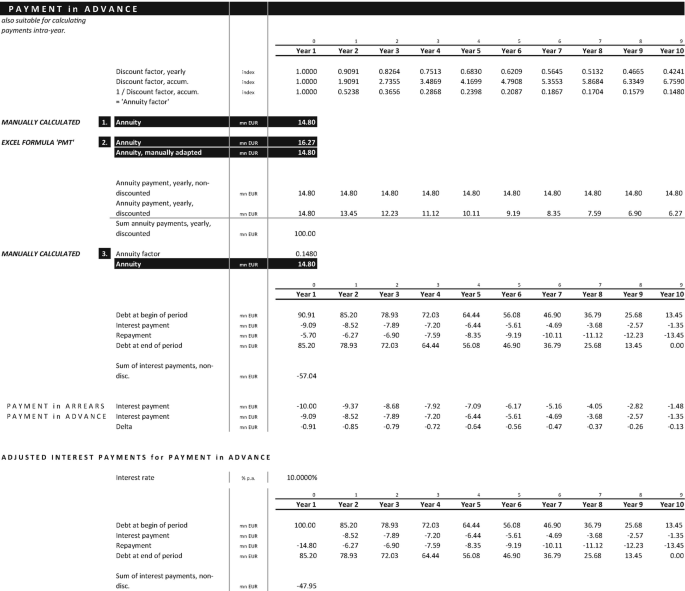
Calculation overview for payment in advance

Bibliography
Literature
Agar, C. (2005). Capital investment & financing: A practical guide to financial evaluation. Elsevier.
Aschauer, E., & Purtscher, V. (2011). Einführung in die Unternehmensbewertung. Wien: Linde.
Ballwieser, W., & Hachmeister, D. (2016). Unternehmensbewertung. Prozess, Methode und Probleme. Stuttgart: Schäffer-Poeschel.
Brealey, R., & Myers, S. (1991). Principles of corporate finance (4th ed.). New York: McGraw-Hill.
Brealey, R., Myers, S., & Allen, F. (2010). Principles of corporate finance (10th ed.pp. 485–486). New York, NY: McGraw-Hill.
Damodaran, A. (2012). Investment valuation: Tools and techniques for determining the value of any asset. Hoboken: Wiley.
Denardo, E. V. (2011). Linear programming and generalizations. Springer.
Dorfman, R., Samuelson, P. A., & Solow, R. M. (1958). Linear programming and economic analysis. New York: McGraw-Hill.
Eayrs, W. E., Ernst, D., & Prexl, S. (2011). Corporate finance training. Stuttgart: Schäffer-Poeschel.
Enzinger, A., & Kofler P. (2011). DCF-Verfahren: Anpassung der Beta-Faktoren zur Erzielung konsistenter Bewertungsergebnisse. RWZ 2011/16, 52–57.
Ernst, D., Schneider, S., & Thielen, B. (2012). Unternehmensbewertungen erstellen und verstehen: Ein Praxisleitfaden. Vahlen.
Ernst, D., Heyd, R., & Popp, M. (2014). Unternehmensbewertung nach IFRS. Berlin: Erich Schmidt Verlag.
Gordon, M. J. (1959). Dividends, earnings, and stock prices. The Review of Economics and Statistics, 41(2), 99–105.
Hamada, R. S. (1972). The effect of the firm’s capital structure on the systematic risk of common stocks. The Journal of Finance, 27(2), 435–452.
Harris R. S., & Pringle, J. J. (1985). Risk-adjusted discount rates – extensions from the average risk case. Journal of Financial Research, 8(3 Fall 1985), 237–244.
Henselmann, K., & Kniest, W. (2015). Unternehmensbewertung: Praxisfälle mit Lösungen. Herne: NWB Verlag.
Kasriel, K., & Wood, D. (2013). Upstream petroleum fiscal and valuation modeling in excel: A worked example. Hoboken: Wiley.
Khinast-Sittenthaler, C. (2015). Unternehmensbewertung in Theorie und Praxis: unter Berücksichtigung des Fachgutachtens KFS/BW 1 2014 (p. 22). Graz: DBV.
Koller, T., Goedhart, M., & Wessels, D. (2015). Valuation: Measuring and managing the value of companies. Hoboken: Wiley.
KPMG. (2016). Cost of capital study 2016: Value measurement – quo vadis? Retrieved from https://assets.kpmg.com/content/dam/kpmg/ch/pdf/cost-of-capital-study-2016-en.pdf
Lüdenbach, N., & Hoffmann, W. D. (Eds.). (2010). Haufe IFRS-Kommentar. Freiburg: Haufe-Lexware.
Miles, J., & Ezzell, J. (1980). The weighted average cost of capital, perfect capital markets and project life: A clarification. Journal of Financial and Quantitative Analysis, 15, 719–730.
Pratt, S. P., & Grabowski, R. J. (2008). Cost of capital: Applications and examples (3rd ed.p. 144). Hoboken, NJ: Wiley.
Rabel, K. (2013). Unternehmensbewertung: Entwurf des neuen Fachgutachtens KFS BW 1. BDO.
Wright, C., & Gallun, R. (2008). Fundamentals of oil & gas accounting. Tulsa: Pennwell Corp.
Author information
Authors and Affiliations
Rights and permissions
Copyright information
© 2018 Springer International Publishing AG, part of Springer Nature
About this chapter

Cite this chapter
Schwarzbichler, M., Steiner, C., Turnheim, D. (2018). Valuation. In: Financial Steering . Springer, Cham. https://doi.org/10.1007/978-3-319-75762-9_5
Download citation
DOI: https://doi.org/10.1007/978-3-319-75762-9_5
Published:
Publisher Name: Springer, Cham
Print ISBN: 978-3-319-75761-2
Online ISBN: 978-3-319-75762-9
eBook Packages: Economics and FinanceEconomics and Finance (R0)