Lattice Vibrations and Thermal Properties

Abstract

Chapter 1 was concerned with the binding forces in crystals and with the manner in which atoms were arranged. Chapter 1 defined, in effect, the universe with which we will be concerned. We now begin discussing the elements of this universe with which we interact. Perhaps the most interesting of these elements are the internal energy excitation modes of the crystals. The quanta of these modes are the “particles” of the solid. This chapter is primarily devoted to a particular type of internal mode—the lattice vibrations.

Problems

• 2.1 Find the normal modes and normal-mode frequencies for a three-atom “lattice” (assume the atoms are of equal mass). Use periodic boundary conditions.

• 2.2 Show when m and m′ are restricted to a range consistent with the first Brillouin zone that

  $$ \frac{1}{N}\sum\limits_{n} {\exp \left( {\frac{{2\pi {\text{i}}}}{N}\left( {m - m^{{\prime }} } \right)n} \right) = \delta_{m}^{{m^{{\prime }} }} } , $$

  where $\delta_{m}^{{m^{{\prime }} }}$ is the Kronecker delta.

• 2.3 Evaluate the specific heat of the linear lattice [given by (2.80)] in the low temperature limit.

• 2.4 Show that G_mn = G_nm, where G is given by (2.100).

• 2.5 This is an essay length problem. It should clarify many points about impurity modes. Solve the five-atom lattice problem shown in Fig. 2.14. Use periodic boundary conditions. To solve this problem define A = β/α and δ = m/M (α and β are the spring constants) and find the normal modes and eigenfrequencies. For each eigenfrequency, plot mω²/α versus δ for A = 1 and mω²/α versus A for δ = 1. For the first plot: (a) The degeneracy at δ = 1 is split by the presence of the impurity. (b) No frequency is changed by more than the distance to the next unperturbed frequency. This is a general property. (c) The frequencies that are unchanged by changing δ correspond to modes with a node at the impurity (M). (d) Identify the mode corresponding to a pure translation of the crystal. (e) Identify the impurity mode(s). (f) Note that as we reduce the mass of M, the frequency of the impurity mode increases. For the second plot: (a) The degeneracy at A = 1 is split by the presence of an impurity. (b) No frequency is changed more than the distance to the next unperturbed frequency. (c) Identify the pure translation mode. (d) Identify the impurity modes. (e) Note that the frequencies of the impurity mode(s) increase with β.

  Fig. 2.14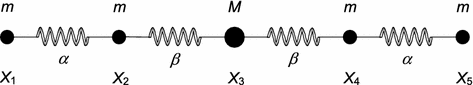

  

  The five-atom lattice

• 2.6 Let a_q and $a_{q}^{\dag }$ be the phonon annihilation and creation operators. Show that

  $$ \left[ {a_{q} ,q_{{q^{1} }} } \right] = 0\quad {\text{and}}\quad \left[ {a_{q}^{\dag } ,a_{{q^{1} }}^{\dag } } \right] = 0. $$

• 2.7 From the phonon annihilation and creation operator commutation relations derive that

  $$ a_{q}^{\dag } \left| {n_{q} } \right\rangle = \sqrt {n_{q} + 1} \left| {n_{q} + 1} \right\rangle , $$

  and

  $$ a_{q} \left| {n_{q} } \right\rangle = \sqrt {n_{q} } \left| {n_{q} - 1} \right\rangle . $$

• 2.8 If a₁, a₂, and a₃ are the primitive translation vectors and if Ω_a = a₁ · (a₂ × a₃), use the method of Jacobians to show that dx dy dz = Ω_a dη₁ dη₂ dη₃, where x, y, z are the Cartesian coordinates and η₁, η₂, and η₃ are defined by r = η₁a₁+ η₂a₂ + η₃a₃.

• 2.9 Show that the b_i vectors defined by (2.172) satisfy

  $$ \varOmega_{a} \varvec{b}_{1} = \varvec{a}_{2} \times \varvec{a}_{3} ,\quad \varOmega_{a} \varvec{b}_{2} = \varvec{a}_{3} \times \varvec{a}_{1} ,\quad \varOmega_{a} \varvec{b}_{3} = \varvec{a}_{1} \times \varvec{a}_{2} , $$

  where Ω_a = a₁ ∙ (a₂ × a₃).

• 2.10 If Ω_b = b₁ · (b₂ × b₃), Ω_a = a₁ · (a₂ × a₃), the b_i are defined by (2.172), and the a_i are the primitive translation vectors, show that Ω_b = 1/Ω_a.

• 2.11 This is a long problem whose results are very important for crystal mathematics. [See (2.178)–(2.184)]. Show that

  • (a)
    $$ \frac{1}{{N_{1} N_{2} N_{3} }}\sum\limits_{{\varvec{R}_{l} }} {\exp \left( {{\text{i}}\varvec{q} \cdot \varvec{R}_{l} } \right) = \sum_{{\varvec{G}_{n} }} \delta_{{\varvec{q},\varvec{G}_{n} }} } , $$

    where the sum over R_l is a sum over the lattice.

  • (b)
    $$ \frac{1}{{N_{1} N_{2} N_{3} }}\sum\limits_{q} {\exp \left( {{\text{i}}\varvec{q} \cdot \varvec{R}_{l} } \right) = \delta_{{\varvec{R}_{l} ,0}} } , $$

    where the sum over q is a sum over one Brillouin zone.

  • (c) In the limit as V_f.p.p. → ∞ (V_f.p.p. means the volume of the parallelepiped representing the actual crystal), one can replace

    $$ \sum\limits_{q} {f\left( \varvec{q} \right)} \quad {\text{by}}\quad \frac{{V_{{{\text{f}} . {\text{p}} . {\text{p}} .}} }}{{\left( {2\pi } \right)^{3} }}\int {f\left( \varvec{q} \right){\text{d}}^{3} \varvec{q}} . $$
  • (d)
    $$ \frac{{\varOmega_{a} }}{{\left( {2\pi } \right)^{3} }}\int\limits_{{{\text{B}} . {\text{Z}} .}} {\exp \left( {{\text{i}}\varvec{q} \cdot \varvec{R}_{l} } \right){\text{d}}^{3} q = \delta_{{\varvec{R}_{l} ,0}} } , $$

    where the integral is over one Brillouin zone.

  • (e)
    $$ \frac{1}{{\varOmega_{a} }}\int {\exp \left[ {{\text{i}}\left( {\varvec{G}_{l ^ {\prime} } - \varvec{G}_{l} } \right) \cdot \varvec{r}} \right]d^{3} r = \delta_{{l^{{\prime }} ,l}} } , $$

    where the integral is over a unit cell.

  • (f)
    $$ \frac{1}{{\left( {2\pi } \right)^{3} }}\int {\exp \left[ {{\text{i}}\varvec{q} \cdot \left( {\varvec{r} - \varvec{r}^{{\prime }} } \right)} \right]{\text{d}}^{3} q = \delta \left( {\varvec{r} - \varvec{r}^{{\prime }} } \right)} , $$

    where the integral is over all of reciprocal space and $\delta$(r − r′) is the Dirac delta function.

  • (g)
    $$ \frac{1}{{\left( {2\pi } \right)^{3} }}\int\limits_{{V_{{{\text{f}} . {\text{p}} . {\text{p}} .}} { \to }\infty }} {\exp \left[ {{\text{i}}\left( {\varvec{q} - \varvec{q}^{{\prime }} } \right) \cdot \varvec{r}} \right]{\text{d}}^{3} r = \delta \left( {\varvec{q} - \varvec{q}^{{\prime }} } \right)} . $$

    In this problem, the a_i are the primitive translation vectors. N₁a₁, N₂a₂, and N₃a₃ are vectors along the edges of the fundamental parallelepiped. R_l defines lattice points in the direct lattice by (2.171). q are vectors in reciprocal space defined by (2.175). The G_l define the lattice points in the reciprocal lattice by (2.173). Ω_a = a₁ · (a₂ × a₃), and the r are vectors in direct space.

• 2.12 This problem should clarify the discussion of diagonalizing H_q (defined by 2.198). Find the normal mode eigenvalues and eigenvectors associated with

  $$ \begin{array}{*{20}c} {m_{i} \ddot{x}_{i} = - \sum\limits_{j = 1}^{3} {\gamma_{ij} x_{j} } ,} \\ {m_{1} = m_{3} = m,\quad m_{2} = M,\quad {\text{and}}\quad \left( {\gamma_{ij} } \right) = \left( {\begin{array}{*{20}c} {k,} & { - k,} & 0 \\ { - k,} & {2k,} & { - k} \\ {0,} & { - k,} & k \\ \end{array} } \right).} \\ \end{array} $$

  A convenient substitution for this purpose is

  $$ x_{i} = u_{i} \frac{{{\text{e}}^{{{\text{i}}\omega t}} }}{{\sqrt {m_{i} } }}. $$

• 2.13 By use of the Debye model, show that

  $$ c_{v} \, { \propto } \, T^{3} \quad {\text{for}}\quad T \ll \theta_{D} $$

  and

  $$ c_{v} { \propto 3}k\left( {NK} \right)\quad {\text{for}}\quad T \gg \theta_{D} . $$

  Here, k = the Boltzmann gas constant, N = the number of unit cells in the fundamental parallelepiped, and K = the number of atoms per unit cell. Show that this result is independent of the Debye model.

• 2.14 The nearest-neighbor one-dimensional lattice vibration problem (compare Sect. 2.2.2) can be exactly solved. For this lattice: (a) Plot the average number (per atom) of phonons (with energies between ω and ω + dω) versus ω for several temperatures. (b) Plot the internal energy per atom versus temperature. (c) Plot the entropy per atom versus temperature. (d) Plot the specific heat per atom versus temperature. [Hint: Try to use convenient dimensionless quantities for both ordinates and abscissa in the plots.]

  

• 2.15 Find the reciprocal lattice of the two-dimensional square lattice shown above.

• 2.16 Find the reciprocal lattice of the three-dimensional body-centered cubic lattice. Use for primitive lattice vectors

  $$ \varvec{a}_{1} = \frac{a}{2}\left( {\hat{\varvec{x}} + \hat{\varvec{y}} - \hat{\varvec{z}}} \right),\quad \varvec{a}_{2} = \frac{a}{2}\left( { - \hat{\varvec{x}} + \varvec{\hat{y} + \hat{z}}} \right),\quad \varvec{a}_{3} = \frac{a}{2}\left( {\hat{\varvec{x}} - \varvec{\hat{y} + \hat{z}}} \right). $$

• 2.17 Find the reciprocal lattice of the three-dimensional face-centered cubic lattice. Use as primitive lattice vectors

  $$ \varvec{a}_{1} = \frac{a}{2}\left( {\hat{\varvec{x}} + \hat{\varvec{y}}} \right),\quad \varvec{a}_{2} = \frac{a}{2}\left( {\varvec{\hat{y} + \hat{z}}} \right),\quad \varvec{a}_{3} = \frac{a}{2}\left( {\varvec{\hat{y} + \hat{x}}} \right). $$

• 2.18 Sketch the first Brillouin zone in the reciprocal lattice of the fcc lattice. The easiest way to do this is to draw planes that perpendicularly bisect vectors (in reciprocal space) from the origin to other reciprocal lattice points. The volume contained by all planes is the first Brillouin zone. This definition is equivalent to the definition just after (2.176).

• 2.19 Sketch the first Brillouin zone in the reciprocal lattice of the bcc lattice. Problem 2.18 gives a definition of the first Brillouin zone.

• 2.20 Find the dispersion relation for the two-dimensional monatomic square lattice in the harmonic approximation. Assume nearest-neighbor interactions.

• 2.21 Write an exact expression for the heat capacity (at constant area) of the two-dimensional square lattice in the nearest-neighbor harmonic approximation. Evaluate this expression in an approximation that is analogous to the Debye approximation, which is used in three dimensions. Find the exact high- and low-temperature limits of the specific heat.

• 2.22 Use (2.200) and (2.203), the fact that the polarization vectors satisfy

  $$ \sum\limits_{p} {e_{{\varvec{q}p\varvec{b}}}^{ * \alpha } e_{{\varvec{q}p\varvec{b}^{{\prime }} }}^{ * \beta } = \delta_{\alpha }^{\beta } \delta_{\varvec{b}}^{{\varvec{b}^{{\prime }} }} } $$

  (the α and β refer to Cartesian components), and

  $$ X_{{ - \varvec{q},p}}^{11\dag } = X_{{\varvec{q},p}}^{11\dag } ,P_{{ - \varvec{q},p}}^{11\dag } = P_{{\varvec{q},p}}^{11} . $$

  (you should convince yourself that these last two relations are valid) to establish that

  $$ {\mathbf{X}}_{{\varvec{q,b}}}^{1} = - {\text{i}}\sum\limits_{p} {\sqrt {\frac{\hbar }{{2m_{\varvec{b}} \omega_{{\varvec{q},p}} }}} \varvec{e}_{{\varvec{q},p,\varvec{b}}}^{ * } \left( {a_{{\varvec{q},p}}^{\dag } - a_{{ - \varvec{q},p}} } \right)} . $$

• 2.23 Show that the specific heat of a lattice at low temperatures goes as the temperature to the power of the dimension of the lattice as in Table 2.5.

• 2.24 Discuss the Einstein theory of specific heat of a crystal in which only one lattice vibrational frequency is considered. Show that this leads to a vanishing of the specific heat at absolute zero, but not as T cubed.

• 2.25 In (2.270) show v_l is longitudinal and v₂, v₃ are transverse.

• 2.26 Derive wave velocities and physically describe the waves that propagate along the [110] directions in a cubic crystal. Use (2.269).