Composing Families of Timed Automata

Abstract

Featured Timed Automata (FTA) is a formalism that enables the verification of an entire Software Product Line (SPL), by capturing its behavior in a single model instead of product-by-product. However, it disregards compositional aspects inherent to SPL development. This paper introduces Interface FTA (IFTA), which extends FTA with variable interfaces that restrict the way automata can be composed, and with support for transitions with atomic multiple actions, simplifying the design. To support modular composition, a set of Reo connectors are modelled as IFTA. This separation of concerns increases reusability of functionality across products, and simplifies modelling, maintainability, and extension of SPLs. We show how IFTA can be easily translated into FTA and into networks of Timed Automata supported by UPPAAL. We illustrate this with a case study from the electronic government domain.

G. Cledou—Supported by the European Regional Development Fund (ERDF) through the Operational Programme for Competitiveness and Internationalisation (COMPETE 2020), and by National Funds through the Portuguese funding agency, FCT, within project POCI-01-0145-FEDER-016826 and FCT grant PD/BD/52238/2013.

J. Proenca—Supported by FCT under grant SFRH/BPD/91908/2012.

L. Barbosa—Supported by the project SmartEGOV: Harnessing EGOV for Smart Governance (Foundations, Methods, Tools)/NORTE-01-0145-FEDER-000037, supported by Norte Portugal Regional Operational Programme (NORTE 2020), under the PORTUGAL 2020 Partnership Agreement, through the European Regional Development Fund (ERDF).

1 Introduction

Software product lines (SPLs) enable the definition of families of systems where all members share a high percentage of common features while they differ in others. Among several formalisms developed to support SPLs, Featured Timed Automata (FTA) [5] model families of real-time systems in a single model. This enables the verification of the entire SPL instead of product-by-product. However, FTA still need more modular and compositional techniques well suited to SPL-based development.

To address this issue, this paper proposes Interface FTA (IFTA), a mechanism enriching FTA with (1) interfaces that restrict the way multiple automata interact, and (2) transitions labelled with multiple actions that simplify the design. Interfaces are synchronisation actions that can be linked with interfaces from other automata when composing automata in parallel. IFTA can be composed by combining their feature models and linking interfaces, imposing new restrictions over them. The resulting IFTA can be exported to the UPPAAL real-time model checker to verify temporal properties, using either a network of parallel automata in UPPAAL, or by flattening the composed automata into a single one. The latter is better suited for IFTA with many multiple actions.

We illustrate the applicability of IFTA with a case study from the electronic government (e-government) domain, in particular, a family of licensing services. This services are present in most local governments, who are responsible for assessing requests and issuing licenses of various types. E.g., for providing public transport services, driving, construction, etc. Such services comprise a number of common functionality while they differ in a number of features, mostly due to specific local regulations.

The rest of this paper is structured as follows. Section 2 presents some background on FTA. Section 3 introduces IFTA. Section 4 presents a set of Reo connectors modeled as IFTA. Section 5 discusses a prototype tool to specify and manipulate IFTA. Section 6 presents the case study. Section 7 discusses related work, and Sect. 8 concludes.

2 Featured Timed Automata

This work builds on top of Featured Timed Automata (FTA) an extension to Timed Automata, introduced by Cordy et al. [5] to verify real-time systems parameterised by a variability model. This section provides an overview of FTA and their semantics, based on Cordy et al.

Informally, a Featured Timed Automaton is an automaton whose edges are enriched with clocks, clock constraints (CC), synchronisation actions, and feature expressions (FE). A clock $c \in C$ is a logical entity that captures the (continuous and dense) time that has passed since it was last reset. When a timed automaton evolves over time, all clocks are incremented simultaneously. A clock constraint is a logic condition over the value of a clock. A synchronisation action $a \in A$ is used to coordinate automata in parallel; an edge with an action a can only be taken when its dual action in a neighbor automaton is also on an edge that can be taken simultaneously. Finally, a feature expression (FE) is a logical constraint over a set of features. Each of these features denotes a unit of variability; by selecting a desired combination of features one can map an FTA into a Timed Automaton.

Fig. 1.

Example of a Featured Timed Automata over the features and .

Figure 1 exemplifies a simple FTA with two locations, $\ell _0$ and $\ell _1$, with a clock c and two features and , standing for the support for brewing coffee and for including milk in the coffee. Initially the automaton is in location $\ell _0$, and it can evolve either by waiting for time to pass (incrementing the clock c) or by taking one of its two transitions to $\ell _1$. The top transition, for example, is labelled by the action coffee and is only active when the feature is present. Taking this transition triggers the reset of the clock c back to 0, evolving to the state $\ell _1$. Here it can again wait for the time to pass, but for at most 5 time units, determined by the invariant $c\le 5$ in $\ell _1$. The transition labelled with brew has a different guard: a clock constraint $c\ge 2$ that allows this transition to be taken only when the clock c is greater than 2. Finally, the lower expression defines the feature model. I.e., how the features relate to each other. In this case the feature can only be selected when the feature is also selected.

We now formalize clock constraints, feature expressions, and the definition of FTA and its semantics.

Definition 1

(Clock Constraints (CC), valuation, and satisfaction). A clock constraint over a set of clocks C, written $g \in CC(C)$ is defined by

where $c \in C$, and $n \in \mathbb {N}$.

A clock valuation $\eta$ for a set of clocks C is a function $\eta :C \rightarrow \mathbb {R}_{\ge 0}$ that assigns each clock $c \in C$ to its current value $\eta c$. We use $\mathbb {R}^C$ to refer to the set of all clock valuations over a set of clocks C. Let $\eta _0(c) = 0$ for all $c \in C$ be the initial clock valuation that sets to 0 all clocks in C. We use $\eta + d$, $d\in \mathbb {R}_{\ge 0}$, to denote the clock assignment that maps all $c \in C$ to $\eta (c) + d$, and let $[r \mapsto 0]\eta$, $r \subseteq C$, be the clock assignment that maps all clocks in r to 0 and agrees with $\eta$ for all other clocks in $C \setminus r$.

The satisfaction of a clock constraint g by a clock valuation $\eta$, written $\eta \models g$, is defined as follows

where $\mathop {\square }\in \{<,\le ,=,>,\ge \}$.

Definition 2

(Feature Expressions (FE) and satisfaction). A feature expression $\varphi$ over a set of features F, written $\varphi \in FE(F)$, is defined by

where $f \in F$ is a feature. The other logical connectives can be encoded as usual: $\bot = \lnot \top$; $\varphi _1 \rightarrow \varphi _2 = \lnot \varphi _1 \vee \varphi _2$; and $\varphi _1 \leftrightarrow \varphi _2 = (\varphi _1 \rightarrow \varphi _2)\wedge (\varphi _2 \rightarrow \varphi _1)$.

Given a feature selection $FS \subseteq F$ over a set of features F, and a feature expression $\varphi \in FE(F)$, FS satisfies $\varphi$, noted $FS \models \varphi$, if

where $\diamondsuit \in \{\wedge , \vee \}$.

Definition 3

(Featured Timed Automata (FTA) [5]). An FTA is a tuple $\mathcal {A} = (L,L_0, A, C,$ $F, E, Inv, fm , \gamma )$ where L is a finite set of locations, $L_0 \subseteq L$ is the set of initial locations, A is a finite set of synchronisation actions, C is a finite set of clocks, F is a finite set of features, E is a finite set of edges, $E \subseteq L \times CC(C) \times A \times \mathbf {2}^{C} \times L$, $Inv: L \rightarrow CC(C)$ is the invariant, a partial function that assigns CCs to locations, $fm \in FE (F)$ is a feature model defined as a Boolean formula over features in F, and $\gamma : E \rightarrow FE (F)$ is a total function that assigns feature expressions to edges.

The semantics of FTA is given in terms of Featured Transition Systems (FTSs) [4]. An FTS extends Labelled Transition Systems with a set of features F, a feature model $fm$, and a total function $\gamma$ that assigns FE to transitions.

Definition 4

(Semantics of FTA). Let $\mathcal {A} = (L,L_0,A,C,F,E, Inv , fm ,\gamma )$ be an FTA. The semantics of $\mathcal {A}$ is defined as an FTS $\langle S, S_0, A, T,F, fm , \gamma ' \rangle$, where $S \subseteq L \times \mathbb {R}^C$ is the set of states, $S_0 = \{\langle \ell _0, \eta _0 \rangle \mid \ell _0 \in L_0\}$ is the set of initial states, $T \subseteq S \times (A \cup \mathbb {R}_{\ge 0}) \times S$ is the transition relation, with $(s_1, \alpha , s_2) \in T$, and $\gamma ' :T \rightarrow FE(F)$ is a total function that assigns feature expressions to transitions. The transition relation and $\gamma$ are defined as follows.

where $s_1 \xrightarrow [ {\varphi } ]{ {\alpha }} s_2$ means that $(s_1, \alpha , s_2) \in T$ and $\gamma (s_1, \alpha , s_2)=\varphi$, for any $s_1,s_2 \in S$.

Notation: We write $L_\mathcal {A}$, ${L_0}_\mathcal {A}$, $A_\mathcal {A}$, etc., to denote the locations, initial locations, actions, etc., of an FTA $\mathcal {A}$, respectively. We write to denote that $(\ell _1,cc,a,c,\ell _2) \in E_\mathcal {A}$, and use to express that $\gamma _\mathcal {A} (\ell _1,cc,a,c,\ell _2) = \varphi$. We omit the subscript whenever automaton $\mathcal {A}$ is clear from the context. We use an analogous notation for elements of an FTS.

3 Interface Featured Timed Automata

Multiple FTAs can be composed and executed in parallel, using synchronising actions to synchronise edges from different parallel automata. This section introduces interfaces to FTA that: (1) makes this implicit notion of communication more explicit, and (2) allows multiple actions to be executed atomically in a transition. Synchronisation actions are lifted to so-called ports, which correspond to actions that can be linked with actions from other automata. Hence composition of IFTA is made by linking ports and by combining their variability models.

Definition 5

(Interface Featured Timed Automata). An IFTA is a tuple $\mathcal {A} = (L,l_0,A,C,F, E, Inv , fm , \gamma )$ where $L, C, F, Inv , fm , \gamma$ are defined as in Featured Timed Automata, there exists only one initial location $l_0$, $A=I\uplus O \uplus H$ is a finite set of actions, where I is a set of input ports, O is a set of output ports, and H is a set of hidden (internal) actions, and edges in E contain sets of actions instead of single actions ($E \subseteq L \times CC(C) \times \underline{\mathbf {2}^{ A }} \times \mathbf {2}^{C} \times L$).

We call interface of an IFTA $\mathcal {A}$ the set $\mathbb {P}_\mathcal {A} = I_\mathcal {A} \uplus O_\mathcal {A}$ of all input and output ports of an automaton. Given a port we write and to denote that is an input or output port, respectively, following the same conventions as UPPAAL for actions, and write instead of when clear from context. The lifting of actions into sets of actions will be relevant for the composition of automata. Notation: we use $i,i_1$, etc., and $o,o_1$, etc. to refer specifically to input and output ports of an IFTA, respectively. For any IFTA $\mathcal {A}$ it is possible to infer a feature expression for each action based on the feature expressions of the edges in which appears. Intuitively, this feature expression determines the set of products requiring .

Definition 6

(Feature Expression of an Action). Given an IFTA $\mathcal {A}$, the feature expression of any action is the disjunction of the feature expressions of all of its associated edges, defined as

We say an IFTA $\mathcal {A}$ is grounded, if it has a total function associating a feature expression to each action that indicates the set of products where was originally designed to be present in. Given an IFTA $\mathcal {A}$ we can construct a grounded $\mathcal {A}$ by incorporating a function $\varGamma$ such that, $\mathcal {A} = (L_\mathcal {A},l_{0_\mathcal {A}},A_\mathcal {A},C_\mathcal {A}, Inv _\mathcal {A},F_\mathcal {A}, fm _\mathcal {A},\gamma _\mathcal {A},\varGamma )$, where $\varGamma : A_\mathcal {A} \rightarrow FE (F_\mathcal {A})$ assigns a feature expression to each action of $\mathcal {A}$, and is constructed based on $\widehat{\varGamma }_\mathcal {A}$. From now on when referring to an IFTA we assume it is a grounded IFTA.

Fig. 2.

Representation of 3 IFTA, depicting their interfaces (blue) and associated feature expressions. (Color figure online)

Figure 2 depicts the interfaces of 3 different IFTA. The leftmost is a payment machine that receives actions representing coins and publishes actions confirming the payment, whose actions are dependent on a feature called . The rightmost is the coffee machine from Fig. 1. Finally, the middle one depicts a connector $Router$ that could be used to combine the payment and the coffee machines. This notion of combining IFTA is the core contribution of this work: how to reason about the modular composition of timed systems with variable interfaces. For example, let us assume the previous IFTA are connected by linking actions as follows: ,, , , and , . In a real coffee machine, after a payment, the machine should allow to select only beverages supported, i.e., if the machine does not support cappuccino the user should not be able to select it and be charged. Similarly, the composed system here should not allow to derive a product with if is not present. To achieve this, we need to impose additional restriction on the variability model of the composed system, since as it will be shown later in this section, combining the feature models of the composed IFTA through logical conjunction is not enough.

The semantics of IFTA is given in terms of FTSs, similarly to the semantics of FTA with the difference that transitions are now labelled with sets of actions. We formalize this as follows.

Definition 7

(Semantics of IFTA). Let $\mathcal {A}$ be an IFTA, its semantics is an FTS $\mathcal {F} = (S, s_0, A, T,F, fm , \gamma )$, where S, A, F, $fm$, and $\gamma$ are defined as in Definition 4, $s_0 = \langle \ell _0,\eta _0 \rangle$ is now the only initial state, and $T \subseteq S \times (\mathbf {2}^{A} \cup \mathbb {R}_{\ge 0}) \times S$ now supports transitions labelled with sets of actions.

We now introduce two operations: product and synchronisation, which are used to define the composition of IFTA. The product operation for IFTA, unlike the classical product of timed automata, is defined over IFTA with disjoint sets of actions, clocks and features, performing their transitions in an interleaving fashion.

Definition 8

(Product of IFTA). Given two IFTA $\mathcal {A} _1$ and $\mathcal {A} _2$, with disjoint actions, clocks and features, the product of $\mathcal {A} _1$ and $\mathcal {A} _2$, denoted $\mathcal {A} _1 \times \mathcal {A} _2$, is

$$\begin{aligned} \mathcal {A} = (L_1 \times L_2, \ell _{0_1} \times \ell _{0_2}, A, C_1 \cup C_2, F_1 \cup F_2, E, Inv , fm _1 \wedge fm _2, \gamma , \varGamma ) \end{aligned}$$

where A, E, $Inv$, $\gamma$ and $\varGamma$ are defined as follows

• $A = I \uplus O \uplus H$, where $I = I_1 \cup I_2$, $O = O_1 \cup O_2$, and $H = H_1 \cup H_2$.

• E and $\gamma$ are defined by the rules below, for any $\omega _1 \subseteq A_1$, $\omega _2 \subseteq A_2$.

  

• $Inv (\ell _1,\ell _2) = Inv _1(\ell _1) \wedge Inv _2(\ell _2)$.

• $\forall ~_{a\in \mathbb {P}_\mathcal {A}} ~\cdot ~ \varGamma (a)= \varGamma _{i}(a)$ if $a \in A_{i}$, for $i=1,2$.

The synchronisation operation over an IFTA $\mathcal {A}$ connects and synchronises two actions a and b from $A_\mathcal {A}$. The resulting automaton has transitions without neither a and b, nor both a and b. The latter become internal transitions.

Definition 9

(Synchronisation). Given an IFTA $\mathcal {A} = (L,\ell _0, A,C, F, E, Inv , fm , \gamma , \varGamma )$ and two actions $a,b \in A$, the synchronisation of a and b is given by $\varDelta _{a,b}(\mathcal {A}) = (L, \ell _0, A', C, F, E', Inv , fm' , \gamma , \varGamma )$ where $A'$, $E'$ and $fm'$ are defined as follows

• $A = I' \uplus O' \uplus H'$, where $I' = I\setminus \{a.b\}$, $O' = O\setminus \{a.b\}$, and $H' = H \cup \{a.b\}$.

• $\begin{array}[t]{@{}l@{~}l@{}} E' =&{} \{\ell \xrightarrow {\;g,\omega , r\;} \ell ' \in E \mid a \notin \omega \text { and } b\notin \omega \} ~ \cup \\ {} &{} \{\ell \xrightarrow {\;g,\omega \backslash \{a,b\}, r\;} \ell ' \mid \ell \xrightarrow {\;g,\omega , r\;} \ell ' \in E \text { and } a\in \omega \text { and }b \in \omega \} \end{array}$

• $fm ^\prime = fm \wedge (\varGamma _\mathcal {A} (a) \leftrightarrow \varGamma _\mathcal {A} (b))$.

Together, the product and the synchronisation can be used to obtain in a compositional way, a complex IFTA modelling SPLs built out of primitive IFTA.

Definition 10

(Composition of IFTA). Given two disjoint IFTA, $\mathcal {A} _1$ and $\mathcal {A} _2$, and a set of bindings $\{(a_1,b_1),\dots ,(a_n,b_n)\}$, where $a_k \in \mathbb {P}_1$, $b_k \in \mathbb {P}_2$, and such that $(a_k,b_k) \in I_1 \times O_2$ or $(a_k,b_k) \in I_2 \times O_1$, for $1\le k \le n$, the composition of $\mathcal {A} _1$ and $\mathcal {A} _2$ is defined as $\mathcal {A} _1 \bowtie _{(a_1, b_1), \dots , (a_n,b_n)} \mathcal {A} _2 = \varDelta _{a_1, b_1}\dots \varDelta _{a_n, b_n}(\mathcal {A} _1 \times \mathcal {A} _2)$.

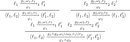
Figure 3 exemplifies the composition of the coffee machine (CM) and Router IFTA from Fig. 2. The resulting IFTA combines the feature models of the CM and Router, imposing additional restrictions given by the binded ports, E.g., the binding (, ) imposes that will be present, if and only if, is present, which depends on the feature expressions of each port, I.e., . In the composed IFTA, transitions with binded actions transition together, while transitions labelled with non-binded actions can transition independently or together. Combining their feature models only through logical conjunction allows as a valid feature selection. In such scenario, we could derive a product that can issue but that can not be captured by . In terms of methods calls in a programming language, the derive product will have a call to a method that does not exists, leading to an error.

Fig. 3.

Composition of a Router IFTA (top left) with the CM IFTA (top right) by binding ports and , yielding the IFTA below.

To study properties of IFTA operations, we define the notion of IFTA equivalence in terms of bisimulation over their underlying FTSs. We formally introduce the notion of timed bisimulation adapted to FTSs.

Definition 11

(Timed Bisimulation). Given two FTSs $\mathcal {F} _1$ and $\mathcal {F} _2$, we say $\mathcal {R} \subseteq S_1 \times S_2$ is a bisimulation, if and only if, for all possible feature selections $FS \in \mathbf {2}^{F_1 \cup F_2}$, $FS \models fm _1 \Leftrightarrow FS \models fm _2$ and for all $(s_1,s_2) \in R$ we have:

• $\forall ~t = s_1 \xrightarrow {\;\alpha \;}_1 s_1'$, $\alpha \in \mathbf {2}^{A} \cup \mathbb {R}_{\ge 0}$, $\exists ~t' = s_2 \xrightarrow {\;\alpha \;}_2 s_2'$ s.t. $(s_1',s_2') \in \mathcal {R}$ and $FS \models \gamma _1(t) \Leftrightarrow FS \models \gamma _2(t')$,

• $\forall ~t' = s_2 \xrightarrow {\;\alpha \;}_2 s_2'$, $\alpha \in \mathbf {2}^{A} \cup \mathbb {R}_{\ge 0}$, $\exists ~t = s_1 \xrightarrow {\;\alpha \;}_1 s_1'$ s.t. $(s_1',s_2') \in \mathcal {R}$ and $FS \models \gamma _1(t) \Leftrightarrow FS \models \gamma _2(t')$

where $A = A_1 \cup A_2$.

Two states $s_1 \in S_1$ and $s_2 \in S_2$ are bisimilar, written $s_1 \sim s_2$, if there exists a bisimulation relation containing the pair $(s_1,s_2)$. Given two IFTA $\mathcal {A} _1$ and $\mathcal {A} _2$, we say they are bisimilar, written $\mathcal {A} _1 \sim \mathcal {A} _2$, if there exists a bisimulation relation containing the initial states of their corresponding FTSs.

Proposition 1

(Product is commutative and associative). Given two IFTA $\mathcal {A} _1$ and $\mathcal {A} _2$ with disjoint set of actions and clocks, $\mathcal {A} _1 \times \mathcal {A} _2 \sim \mathcal {A} _2 \times \mathcal {A} _1$, and $\mathcal {A} _1 \times (\mathcal {A} _2 \times \mathcal {A} _3) \sim (\mathcal {A} _1 \times \mathcal {A} _2) \times \mathcal {A} _3$.

The proof follows trivially by definition of product and FTSs, and because $\cup$ and $\wedge$ are associative and commutative.

The synchronisation operation is commutative, and it interacts well with product. The following proposition captures these properties.

Proposition 2

(Synchronisation commutativity). Given two IFTA $\mathcal {A} _1$ and $\mathcal {A} _2$, the following properties hold:

• 1. $\varDelta _{a,b}\varDelta _{c,d}\mathcal {A} _1 \sim \varDelta _{c,d}\varDelta _{a,b}\mathcal {A} _1$, if $a,b,c,d \in A_1$, a, b, c, d different actions.

• 2. $(\varDelta _{a,b}\mathcal {A} _1) \times \mathcal {A} _2 \sim \varDelta _{a,b}(\mathcal {A} _1 \times \mathcal {A} _2)$, if $a,b \in A_1$ and $A_1 \cap A_2 = \emptyset$.

Both proof follow trivially by definition of product, synchronization and FTSs.

4 Reo Connectors as IFTA

Reo is a channel-based exogenous coordination language where complex coordinators, called connectors, are compositionally built out of simpler ones, called channels [2]. Exogenous coordination facilitates anonymous communication of components. Each connector has a set of input and output ports, and a formal semantics of how data flows from the inputs to the outputs. We abstract from the notion of data and rather concentrate on how execution of actions associated to input ports enables execution of actions associated to output ports.

Table 1 shows examples of basic Reo connectors and their corresponding IFTA. For example, Merger $(i_1,i_2,o)$ synchronises each input port, separately, with the output port, i.e. each $i_k$ executes simultaneously with o for $k=1,2$; and FIFO1(i, o) introduces the notion of delay by executing its input while transitions to a state where time can pass, enabling the execution of its output without time restrictions.

Modelling Reo connectors as IFTA enables them with variable behavior based on the presence of ports connected through synchronisation to their ports. Thus, we can use them to coordinate components with variable interfaces. We associate a feature to each port of a connector and define its behavior in terms of these features. Table 1 shows Reo basic connectors as IFTA with variable behavior. Bold edges represent the standard behavior of the corresponding Reo connector, and thinner edges model variable behavior. For example, the Merger connector supports the standard behavior, indicated by the transitions $k=1,2$ and the corresponding feature expression ; and a variable behavior, in which both inputs can execute independently at any time if is not present, indicated by transitions $k=1,2$ and the corresponding feature expression .

Table 1. Examples of basic Reo connectors and their corresponding IFTA.

The Sync connector behaves as the identity when composed with other automata. The following proposition captures this property.

Proposition 3

( Sync behaves as identity). Given an IFTA $\mathcal {A}$ and a Sync connector, $\varDelta _{i,a}(\mathcal {A} \times Sync (i,o)) \sim \mathcal {A} [o/a]$ with the following updates

• $fm _{\mathcal {A} [o/a]} = fm _\mathcal {A} \wedge (f_{io} \leftrightarrow \varGamma _\mathcal {A} (a))$

• , if $o \in \omega$

• $F_{\mathcal {A} [o/a]} = F_\mathcal {A} \cup \{f_{io}\}$

• $\varGamma _{\mathcal {A} [o/a]}(o) = \varGamma _{ Sync }(o)$

if $\{i,o\} \not \subseteq A_\mathcal {A}$, and $a \in A_\mathcal {A}$. $\mathcal {A} [o/a]$ is $\mathcal {A}$ with all occurrences of a replaced by o.

Proof

First for simplicity, let $\mathcal {A} _S = (\mathcal {A} \times Sync (i,o))$, and $\mathcal {A} ' = \varDelta _{i,a}(\mathcal {A} _S)$. Lets note that the set of edges in $\mathcal {A} '$ is defined as follows

where $\ell _0$ is the initial and only location of Sync. Let $\mathcal {F} _1$ and $\mathcal {F} _2$ be the underlying FTS of $\mathcal {A} '$ and $\mathcal {A} [o/a]$, and note that $\mathcal {R} = \{(\langle (\ell _1,\ell _0),\eta \rangle , \langle \ell _1,\eta \rangle ) ~|~ \ell _1 \in S_{\mathcal {A} [o/a]} \}$ is a bisimulation between states of $\mathcal {F} _1$ and $\mathcal {F} _2$. Let $(\langle (\ell _1,\ell _0),\eta \rangle ,\langle \ell _1,\eta \rangle ) \in \mathcal {R}$. The proof for delay transitions follows trivially from the fact that $Inv (\ell _1,\ell _0) = Inv (\ell _1)$ for all $\ell _1 \in S_{\mathcal {A} [o/a]}$.

Lets consider any action transition $\langle (\ell _1,\ell _0),\eta \rangle \xrightarrow {\;\omega \;} \langle (\ell '_1, \ell _0),\eta ' \rangle \in T_{\mathcal {F} _1}$. If it comes from an edge in (1), then $\exists ~\ell _1 \xrightarrow {\;g,\omega ,r\;} \ell '_1 \in E_\mathcal {A} ~ s.t. ~ a \not \in \omega$, thus $\exists ~\langle \ell _1,\eta \rangle \xrightarrow {\;\omega \;} \langle \ell '_1,\eta ' \rangle \in T_{\mathcal {F} _2}$; if it comes from (2), then $\exists ~\ell _1 \xrightarrow {\;g,\omega _1,r\;} \ell '_1 \in E_\mathcal {A} ~ s.t. ~ a \in \omega _1$, thus $\exists ~\langle \ell _1,\eta \rangle \xrightarrow {\;\omega _1{[o/a]}\;} \langle \ell '_1,\eta ' \rangle \in T_{\mathcal {F} _2}$, where $\omega = \omega _1 \cup \{i,o\} \setminus \{i,a\} = \omega [o/a]$. Conversely, if $\exists ~\langle \ell _1,\eta \rangle \xrightarrow {\;\omega \;} \langle \ell '_1,\eta ' \rangle \in T_{\mathcal {F} _2}$ and $o \not \in \omega$, then $\exists ~(\ell _1,\ell _0) \xrightarrow {\;g,\omega ,r\;} (\ell '_1, \ell _0) \in E_{\mathcal {A} _S} ~ s.t. ~ i \notin \omega \wedge a \notin \omega$, thus $\exists ~\langle (\ell _1,\ell _0), \eta \rangle \xrightarrow {\;\omega \;} \langle (\ell '_1,\ell _0), \eta ' \rangle \in T_{\mathcal {F} _1}$; if $o \in \omega$, then $\exists ~(\ell _1,\ell _0) \xrightarrow {\;g,\omega _1 \cup \{o\} \setminus \{a\},r\;} (\ell '_1,\ell _0) \in E_{\mathcal {A} '}$, such that $\omega = \omega _1[o/a] = \omega _1\cup \{o\} \setminus \{a\}$, thus $\exists ~\langle (\ell _1,\ell _0),\eta \xrightarrow {\;\omega \;} \langle (\ell '_1,\ell _0),\eta ' \rangle \rangle \in T_{\mathcal {F} _1}$.

In both cases, we have $\gamma _{\mathcal {F} _1}(\langle (\ell _1,\ell _0),\eta \rangle \xrightarrow {\;\omega \;} \langle (\ell '_1, \ell _0),\eta ' \rangle ) = \gamma _{\mathcal {F} _2}(\langle \ell _1,\eta \rangle \xrightarrow {\;\omega \;} \langle \ell '_1,\eta ' \rangle )$. Furthermore, $fm _\mathcal {A} ' = fm _{\mathcal {A} [o/a]}$.    $\square$

5 Implementation

We developed a prototype tool in Scala¹ consisting of a small Domain Specific Language (DSL) to specify (networks of) (N)IFTA and manipulate them. Although we do not provide the formal definitions and semantics due to space constraints, informally, a network of any kind of automata is a set of automata parallel composed (||) and synchronised over a set of shared actions.

Main features supported by the DSL include: (1) specification of (N)IFTA, (2) composition, product and synchronisation over IFTA, (3) conversion of NIFTA to networks of FTA (NFTA) with committed states (CS), and (4) conversion of NFTA to UPPAAL networks of TA (NTA) with features. Listing 1.1 shows how the router connector from Table 1 can be specified using the DSL. A comprehensive list of functionality and more examples, including the case study from Sect. 6 can be found in the tool’s repository (see footnote 1).

A NIFTA can be converted into a NFTA with committed states, which in turn can be converted into a network of UPPAAL TA, through a stepwise conversion, as follows. NIFTA to NFTA. Informally, this is achieved by converting each transition with set of actions into to a set of transitions with single actions. All transitions in this set must execute atomically (committed states between them) and support all combinations of execution of the actions. NFTA to UPPAAL NTA. First, the NFTA obtained in the previous step is translated into a network of UPPAAL TA, where features are encoded as Boolean variables, and transition’s feature expressions as logical guards over Boolean variables. Second, the feature model of the network is solved using a SAT solver to find the set of valid feature selections. This set is encoded as a TA with an initial committed location and outgoing transitions to new locations for each element in the set. Each transition initializes the set of variables of a valid feature selection. The initial committed state ensures a feature selection is made before any other transition is taken.

When translating IFTA to FTA with committed states, the complexity of the model grows quickly. For example, the IFTA of a simple replicator with 3 output ports consists of a location and 8 transitions, while its corresponding FTA consists of 23 locations and 38 transitions. Without any support for composing variable connectors, modelling all possible cases is error prone and it quickly becomes unmanageable. This simplicity in design achieved through multi-action transitions leads to a more efficient approach to translate IFTA to UPPAAL TA, in particular by using the composition of IFTA. The IFTA resulting from composing a network of IFTA, can be simply converted to an FTA by flattening the set of actions in to a single action, and later into an UPPAAL TA.

6 Case Study: Licensing Services in E-Government

This section presents a case study of using IFTA to model a family of public licensing services. All services in the family support submissions and assessment of licensing requests. Some services, in addition, require a fee before submitting (), others allow appeals on rejected requests (), or both. Furthermore, services that require a fee can support credit card () or PayPal payments (), or both. Functionality is divided in components and provided as follows. Each component can be visualized in Fig. 4. We omit the explicit illustration of interfaces and rather use the notation , to indicate whether an action corresponds to an input or output, respectively. In addition, we use the same action name in two different automata to indicate pairs of actions to be linked. The feature model, also omitted, is initially for each of these IFTA.

App - Models licenses requests. An applicant must submit the required documents (), and pay a fee () if is present, before submitting (). If the request is accepted () or considered incomplete (), the request is closed. If it is rejected () and it is not possible to appeal (), the request is closed, otherwise a clock ($tapl$) is reseted to track the appeal window time. The applicant has 31 days to appeal ($Inv_{ App }(\ell _5)$), otherwise the request is canceled () and closed. If an appeal is submitted (), it can be rejected or accepted, and the request is closed.

CC and PP - Handle payments through credit cards and PayPal, respectively. If a user requests to pay by credit card () or PayPal (), a clock is reset to track payment elapsed time ($tocc$ and $topp$). The user has 1 day ($Inv_{CC}(\ell _1)$ and $Inv_{PP}(\ell _1)$) to proceed with the payment which can result in success ( and ) or cancellation ( and ).

Appeal - Handles appeal requests. When an appeal is received (), a clock is reseted to track the appeal submission elapsed time ($tas$). Authorities have 20 days ($Inv _{Appeal}(\ell _1)$) to start assessing the request ().

Preassess - Checks if a request contains all required documents. When a request is received (), a clock is reseted to track the submission elapsed time ($ts$). Authorities have 20 days ($Inv _{Preasses}(\ell _1)$) to check the completeness of the documents and notify whether it is incomplete () or ready to assessed ().

Assess - Analyzes requests. When a request is ready to be assessed (), a clock is reseted to track the processing elapsed time ($tp$). Authorities have 90 days to make a decision of weather accept it () or reject it ().

Fig. 4.

IFTA modelling domain functionality.

Fig. 5.

IFTA for a family of Licensing Services

We use a set of Reo connectors to integrate these IFTA. The final integrated model can be seen in Fig. 5. For simplicity, we omit the feature expressions associated to ports and the resulting feature model. Broadly, we can identify two new components in this figure: Payment - (right of App) Orchestrates payment requests based on the presence of payment methods. It is composed by components CC, PP, and a set of connectors. A router synchronises payment requests () with payment by CC or PayPal ( or ). A merger synchronises the successful response ( or ), while other merger synchronises the cancellation response ( or ) from either CC or PP. On top of the composed feature model, we add the restriction to ensure payment is supported, if and only if, Credit card or PayPal are supported; and Processing - (left of App) Orchestrates the processing of licenses requests and appeals (if is present). It is composed by Appeal, Preassess, Assess, a set of trivial sync connectors and a merger that synchronises assessment requests from either Appeal or Preassess ( or ) with Assess ().

By using IFTA, connectors are reused and it is simple to create complex connectors out of simple ones. If in the future a new payment methods is supported, the model can be updated by simple using a three output replicator and two three inputs mergers. By composing the future model and inferring new restrictions based on how interfaces are connected, it is possible to reason about the variability of the entire network, E.g., we can check if the resulting feature model satisfies variability requirements or if the interaction of automata is consistent with the presence of features. In addition, by using the DSL we can translate this components to UPPAAL to verify properties such as: Deadlock free – A[] not deadlock; Liveness – a submission and an appeal will eventually result in an answer ( and , respectively); Safety – a submission must be processed within 110 days (A[] App. $\ell _4$ imply App.tsub<=110).

7 Related Work

Related work is discussed following two lines: (1) compositionality and modularity of SPLs, and (2) compositionality and interfaces for automata.

Compositionality and modularity of SPLs. An extension to Petri Nets, Feature Nets (FNs) [11] enables specifying the behavior of an SPL in a single model, and supports composition of FNs by applying deltas FNs to core FNs. An extension to CCS process calculus consisting on a modular approach to modelling and verifying variability of SPLs based on DeltaCCS [9]. A compositional approach for verification of software product lines [10] where new features and variability may be added incrementally, specified as finite state machines with variability information.

Interfaces and compositionality of automata. Interface automata [1] use input interfaces to support incremental design and independent implementability of components, allowing compatibility checking of interfaces for partial system descriptions, without knowing the interfaces of all components, and separate refinement of compatible interfaces, respectively. [6] presents a specification theory for I/O TA supporting refinement, consistency checking, logical and structural composition, and quotient of specifications. In [8] Modal I/O automata are used to construct a behavioral variability theory for SPL development and can serve to verify if certain requirements can be satisfied from a set of existing assets. [7] proposes a formal integration model based on Hierarchical TA for real time systems, with different component composition techniques. [3] presents a compositional specification theory to reason about components that interact by synchronisation of I/O actions.

8 Conclusions

This paper introduced IFTA, a formalism for modelling SPL in a modular and compositional manner, which extends FTA with variable interfaces to restrict the way automata can be composed, and with multi-action transitions that simplify the design. A set of Reo connectors were modeled as IFTA and used to orchestrate the way various automata connect. We discussed a prototype tool to specify and manipulate IFTA, which takes advantage of IFTA composition to translate them into TA that can be verified using the UPPAAL model checker.

Delegating coordination aspects to connectors enables separation of concerns. Each automata can be designed to be modular and cohesive, facilitating the maintenance, adaptability, and extension of an SPL. In particular, by facilitating compositional reasoning when replacing components, E.g., when checking for a refinement relation, as well as enabling changes in the coordination mechanisms without affecting core domain functionality. Using bare FTA for designing variable connectors, can be error prone and it quickly becomes unmanageable. IFTA simplifies this design by enabling the modeling of automata in isolation and composing them by explicitly linking interfaces and combining their feature models.

Future work includes studying an implementation relation, I.e, refinement, to reason about how to safely replace an IFTA with a more detailed one in a compose environment.

References

de Alfaro, L., Henzinger, T.A.: Interface automata. SIGSOFT Softw. Eng. Notes 26(5), 109–120 (2001). http://doi.acm.org/10.1145/503271.503226
Arbab, F.: Reo: a channel-based coordination model for component composition. Math. Struct. Comp. Sci. 14(3), 329–366 (2004). http://dx.doi.org/10.1017/S0960129504004153
Chen, T., Chilton, C., Jonsson, B., Kwiatkowska, M.: A compositional specification theory for component behaviours. In: Seidl, H. (ed.) ESOP 2012. LNCS, vol. 7211, pp. 148–168. Springer, Heidelberg (2012). doi:10.1007/978-3-642-28869-2_8
Classen, A., Heymans, P., Schobbens, P.Y., Legay, A.: Symbolic model checking of software product lines. International Conference on Software Engineering, ICSE, pp. 321–330 (2011). http://dl.acm.org/citation.cfm?id=1985838
Cordy, M., Schobbens, P.Y., Heymans, P., Legay, A.: Behavioural modelling and verification of real-time software product lines. In: Proceedings of the 16th International Software Product Line Conference, SPLC 2012, vol. 1. pp. 66–75. ACM, New York (2012). http://doi.acm.org/10.1145/2362536.2362549
David, A., Larsen, K.G., Legay, A., Nyman, U., Wasowski, A.: Timed i/o automata: a complete specification theory for real-time systems. In: Proceedings of the 13th ACM International Conference on Hybrid Systems: Computation and Control, HSCC 2010, pp. 91–100. ACM, New York (2010). http://doi.acm.org/10.1145/1755952.1755967
Jin, X., Ma, H., Gu, Z.: Real-time component composition using hierarchical timed automata. In: Seventh International Conference on Quality Software (QSIC 2007), pp. 90–99, October 2007
Larsen, K.G., Nyman, U., Wąsowski, A.: Modal I/O automata for interface and product line theories. In: De Nicola, R. (ed.) ESOP 2007. LNCS, vol. 4421, pp. 64–79. Springer, Heidelberg (2007). doi:10.1007/978-3-540-71316-6_6
Lochau, M., Mennicke, S., Baller, H., Ribbeck, L.: Incremental model checking of delta-oriented software product lines. J. Logic Algebraic Program. 85(1, Part 2), 245–267 (2016). http://dx.doi.org/10.1016/j.jlamp.2015.09.004, Formal Methods for Software Product Line Engineering
Millo, J.-V., Ramesh, S., Krishna, S.N., Narwane, G.K.: Compositional verification of software product lines. In: Johnsen, E.B., Petre, L. (eds.) IFM 2013. LNCS, vol. 7940, pp. 109–123. Springer, Heidelberg (2013). doi:10.1007/978-3-642-38613-8_8
Muschevici, R., Proença, J., Clarke, D.: Feature nets: behavioural modelling of software product lines. Softw. Syst. Model. 15(4), 1181–1206 (2016). http://dx.doi.org/10.1007/s10270-015-0475-z
Author information
Authors and Affiliations
Corresponding author
Editor information
Editors and Affiliations
Rights and permissions
Copyright information
© 2017 IFIP International Federation for Information Processing
About this paper
Cite this paper
Cledou, G., Proença, J., Soares Barbosa, L. (2017). Composing Families of Timed Automata. In: Dastani, M., Sirjani, M. (eds) Fundamentals of Software Engineering. FSEN 2017. Lecture Notes in Computer Science(), vol 10522. Springer, Cham. https://doi.org/10.1007/978-3-319-68972-2_4
Download citation
DOI: https://doi.org/10.1007/978-3-319-68972-2_4
Published:
Publisher Name: Springer, Cham
Print ISBN: 978-3-319-68971-5
Online ISBN: 978-3-319-68972-2
eBook Packages: Computer ScienceComputer Science (R0)