Primary Production

Lewandowski, I.; Lippe, M.; Montoya, J. Castro; Dickhöfer, U.; Langenberger, G.; Pucher, J.; Schließmann, U.; Schmid-Staiger, U.; Derwenskus, F.; Lippert, C.

doi:10.1007/978-3-319-68152-8_6

I. Lewandowski²,
M. Lippe³,
J. Castro Montoya⁴,
U. Dickhöfer⁴,
G. Langenberger⁵,
J. Pucher⁶,
U. Schließmann⁷,
U. Schmid-Staiger⁷,
F. Derwenskus⁸ &
…
C. Lippert⁹

32k Accesses
5 Citations

An erratum to this publication is available online at https://doi.org/10.1007/978-3-319-68152-8_13

Abstract

Agricultural Production: Agriculture is the cultivation of crops or the husbandry of livestock in pure or integrated crop/animal production systems for the main purpose of food production, but also for the provision of biomass for material and energetic use. Together with forestry, agricultural production represents the main activity of resource production and supply in the bioeconomy and the major activity delivering food as well as starch, sugar and vegetable oil resources. Today, 33% (about 4900 Mha) of the Earth’s land surface is used for agricultural production, providing a living for 2.5 billion people. Agriculture shapes cultural landscapes but, at the same time, is associated with degradation of land and water resources and deterioration of related ecosystem goods and services, is made responsible for biodiversity losses and accounts for 13.5% of global greenhouse gas emissions (IPCC 2006).

In the future bioeconomy, agriculture needs to be performed sustainably. ‘Sustainable intensification’ aims at shaping agricultural production in such a way that sufficient food and biomass can be produced for a growing population while, at the same time, maintaining ecosystem functions and biodiversity. Sustainable intensification can partly be achieved by the development and implementation of innovative production technologies, which allow a more efficient use of natural resources, including land and agricultural inputs. Its implementation requires a knowledge-based approach, in which farmers are made aware of the requirements of sustainable production and trained in the implementation of sustainable agricultural production systems.

The planning of bio-based value chains and sustainable bioeconomic development demands an understanding of the mechanisms of biomass production and supply (as described in this chapter) for the entire global agricultural sector.

Forestry: Forests cover about 30% of the Earth’s total land area, harbouring most of the world’s terrestrial biodiversity and containing almost as much carbon as the atmosphere. They have many functions, providing livelihoods for more than a billion people, and are of high relevance for biodiversity conservation, soil and water protection, supply of wood for energy, construction and other applications, as well as other bio-based resources and materials such as food and feed. The forestry sector was the first to adopt a sustainability concept (cf. Carlowitz), and sustainable use and management of forestry remains an important issue to this day. Forestry is a multifunctional bioeconomic system and has an important function in securing the sustainable resource base for the present and future bioeconomy.

Aquatic Animal Production: Aquatic animals are fundamental to a well-balanced, healthy human diet due to their profile and content of essential amino acids, polyunsaturated fatty acids, vitamins and minerals. Since the 1990s, the growing demand for aquatic food cannot be satisfied by capture fisheries alone and has therefore caused a steady increase in aquaculture production of on average 8.8% annually. Today aquaculture is the fastest-growing agricultural sector globally, especially in Asia. There are 18.7 million fish farmers globally, and annual aquaculture production is worth around 150 billion euros. It is expected that aquaculture will increasingly contribute to protein supply and healthy nutrition of the growing world population.

Fish production can be performed at different intensity levels, from production systems based on natural feed resources to closed systems in ponds or tanks which fully rely on external feed. New integrated aquaculture systems are increasingly being developed and applied, which follow a more direct implementation of a circular bioeconomy and focus on a more efficient use of nutrients and water. The best choice of production method largely depends on local conditions.

Microalgae: Microalgae are one of the most important global biomass producers and can be used commercially to produce specific food, feed and biochemical compounds. The cultivation process differs completely from that of land-based plants because they are grown under more or less controlled conditions in different types of bioreactor systems in salt, brackish or fresh water. Special processing requirements apply to the extraction of valuable compounds from algae biomass and further use of the residual biomass, especially in cascade utilization. In general, the chemical characteristics and market specifications, for example the required degree of product purity, determine the downstream processing technique. Additional requirements are the avoidance of an energy-intensive drying step wherever possible and the ensuring of gentle extraction processes that both maintain the functionality of biochemical compounds and permit the extraction of further cell components.

The vast number of microalgae strains differ fundamentally in cell size, cell wall formation and biomass composition. By applying successive extraction procedures, both the principal fractions (e.g. proteins, polar membrane lipids with omega-3 fatty acids, non-polar triacylglycerides) as well as high-value components such as carotenoids can be obtained sequentially from the microalgae biomass.

Economics of Primary Production: When developing new bio-based products and assessing their market opportunities, the correct calculation of all expected unit costs is indispensable. The provision of natural resources from primary agricultural or forest production is an important cost component in this calculation. All renewable natural resources require a certain time to grow. For this reason, in order to correctly account for all external and internal net benefits of natural resources, it is important to calculate the related capital costs and model the biological growth over time. For permanent crops and woodland resources, it is particularly important to derive optimized single and infinite rotations for different kinds of plantations. For this purpose, the corresponding biological growth expectations need to be combined with an investment appraisal. This chapter introduces basic concepts dealing with interest calculation based on the existence of (economic) capital growth and biological growth.

The original online version of this chapter was revised. An erratum to this chapter can be found at https://doi.org/10.1007/978-3-319-68152-8_13.

Individual section’s authors are indicated on the corresponding sections.

You have full access to this open access chapter, Download chapter PDF

Step-By-Step Along the Path to Sustainability

Agricultural Bioenergy Production

Land-Use Change and Food Supply

Keywords

Primary production is the synthesis of organic substances by autotrophic organisms from atmospheric or aqueous carbon dioxide (CO₂) (see Sect. 5.1). Primary productivity, which is the rate at which energy is converted into organic substances, depends on internal (genetic) and external (ecophysiological) factors. Figure 6.1 shows that the net primary production of biomass is highest in regions where high temperatures are combined with a good water supply and is totally absent in desert regions without a natural water supply.

Apart from light and water, there are other factors that determine primary productivity, including the availability of plant nutrients, mainly nitrogen (N), potassium (K) and phosphorus (P) (Fig. 5.3). The lack of any one of these factors can hinder biomass growth. Unfavourable site conditions, such as soil contamination or compaction, can also impair biomass growth. Because the process of photosynthesis consumes CO₂, potential biomass productivity increases with increasing atmospheric CO₂ concentrations. However, this additional stimulus cannot be transformed into higher productivity if water supply is limited by drought. That means the highest biomass growth is achieved when all factors affecting growth are at their relative optimum.

Primary productivity also differs depending on the type of plant or organism and its genetics. An example of this can be seen in the productivity of ‘C3’ and ‘C4’ plants. Most crops cultivated in temperate climates possess the C3 photosynthetic mechanism, so called because the first product of carbon fixation contains three carbon atoms. Wheat, sugar beet and trees are examples of C3 crops. Carbon fixation in the photosynthesis pathway of C4 crops results in a first product containing four carbon atoms. Sugar cane and other subtropical and tropical crops belong to this group. Under favourable environmental conditions, especially high temperatures, C4 crops are more productive than C3 crops because they possess a more effective biochemical mechanism of fixing CO₂. The genetic component of productivity can be exemplified by the breeding progress achieved in recent decades. It is presumed that the major proportion of yield increases seen in the agricultural crops wheat, rice and maize are the result of intensive breeding. Improved crop management, especially fertilization and crop protection, is the second most important factor driving yield increases.

Actual biomass production very much depends on the kind of land use (see Fig. 6.2). The highest productivity is generally achieved on intensively managed cropland with natural vegetation generally having the lowest.

It is anticipated that a growing bioeconomy will require an increasing supply of biomass. However, not all of the biomass produced can be made available for use. For example, in the context of bioenergy development, there is an ongoing debate about biomass availability and whether the energetic and material use of biomass is in conflict with food supply.

The question of how much biomass can be sustainably used for human consumption, especially for bioenergy, has led to various biomass potential analyses being performed. Several global biomass potential assessments indicate that an additional biomass potential exists for material or energetic application that could be used without jeopardizing food supply (Dornburg et al. 2010; Piotrowski et al. 2015; Smeets et al. 2007). The methods applied in these studies are generally supply-driven, which means they assess biomass potentials on the basis of resources available for biomass production. These resources are either additional land or land that can be more efficiently used to increase biomass productivity. Other supply-driven studies assess and quantify potential biomass supply from untapped or underutilized resources, such as agricultural and forestry residues, landscape and grassland biomass and other organic wastes.

Today, it is generally agreed upon that biomass potential assessment studies should follow the following rules (see also Dornburg et al. 2010):

They should only consider biomass that is not required now or in future for the purpose of food production. A biomass potential should only be indicated as such if it can be generated in addition to products from primary production needed for food or feed purposes.
Biomass should not be produced in any areas of high conservation value (HCV). The Roundtable on Sustainable Palm Oil (RSPO) defines HCVs as ‘… biological, ecological, social or cultural values which are considered outstandingly significant or critically important, at the national, regional or global level. All natural habitats possess inherent conservation values, including the presence of rare or endemic species, provision of ecosystem services, sacred sites, or resources harvested by local residents. An HCV is a biological, ecological, social or cultural value of outstanding significance or critical importance’ (RSPO 2016).

Biomass should not be produced where it would lead to the destruction of high-carbon land-use systems, such as peat, natural forest or permanent grasslands.
Biomass should be generated from the more efficient use of existing agricultural land and sustainable extraction from natural forests or other land-use forms. In addition, more efficient use should be made of existing biomass resources, for example, through more efficient biomass conversion techniques, and of residue streams to increase the biomass potential.

Recent studies have resulted in global biomass potentials ranging from 0 to more than 1100 GJ (Dornburg et al. 2010). The background assumptions applied in the modelling approach form the major determinant of the size of the biomass potential given. There are many factors that determine the sustainably usable biomass potential (Smeets et al. 2007; Dornburg et al. 2010) including:

The local diet, mainly the kind and amount of meat and dairy products consumed. The biomass potential decreases with an increase in the amount of meat consumed because meat production requires 3–100 times more land than crop production (Smeets et al. 2007).
The type and efficiency of meat production. The efficiency of meat production, expressed in terms of kg meat produced per kg feed, differs between animals, regions, feeding systems and others (see Sect. 6.1.10, Table 6.5).
The efficiency of agricultural land use. The actual exploitation of agricultural land, indicated by the proportion of potential yield that is actually harvested, varies widely between countries. It can be close to full exploitation in industrial countries but as low as 30% in African countries (Fig. 6.2). Because biomass potentials are generally assessed by multiplying the respective yield by the amount of land available, the yield assumed is also a major determinant of biomass potentials.
The amount and quality of land considered available for biomass production. The amount of land that is additionally available for biomass production is currently a topic of ongoing debate. The FAO (2002) estimated an untapped potential of 25 billion ha of agricultural land for rainfed biomass production (see also Fig. 6.2). However, large parts of these areas may be characterized as ‘marginal land’. Marginal production conditions can be defined in economic and biophysical terms (Dauber et al. 2012). Biophysical constraints to agricultural production include degradation though erosion, contamination, stoniness, and shallow soils and soils of low fertility. If marginal land is defined as land that does not support economically viable agricultural production, the status of marginality will depend on land-use and biomass prices. A caveat to the use of economically marginal land is the fact that the production of whatever biomasses, be it for food or energetic and material uses, on this land will result in low profit.
The kind of biomass being considered. Lignocellulosic crops, such as trees and grasses, deliver the highest biomass and energy yields per hectare. Many potential studies (Hoogwijk et al. 2005; Smeets et al. 2007) are based on the assumption that short rotation coppice is grown on land available for biomass production. However, a number of material applications and liquid biofuel production require vegetable oils, sugar or starch. These can only be produced at lower yield levels.

These bio-based resources are produced on a land area of 14,900 million ha (Mha) globally, of which 1500 Mha are arable land, 4100 Mha are permanent grassland and pastures and 3900 Mha are forest (Fig. 6.3).

Agriculture and forestry are the largest primary production sectors, followed by fishery, aquaculture and production of algae and microorganisms. Each of these primary sectors forms an important part of the bioeconomy. They are described in the following sections.

1 Agricultural Production

Iris Lewandowski,
Melvin Lippe,
Joaquin Castro Montoya &
Uta Dickhöfer

Institute of Crop Sciences; Biobased Products and Energy Crops, University of Hohenheim, Stuttgart, Germany
Iris Lewandowski
Thünen Institute of International Forestry and Forest Economics, Hamburg, Germany
Melvin Lippe
Institute of Agricultural Sciences in the Tropics; Animal Nutrition and Rangeland Management in the Tropics and Subtropics, University of Hohenheim, Stuttgart, Germany
Joaquin Castro Montoya & Uta Dickhöfer

Abstract

Agriculture is the cultivation of crops or the husbandry of livestock in pure or integrated crop/animal production systems for the main purpose of food production, but also for the provision of biomass for material and energetic use. Together with forestry, agricultural production represents the main activity of resource production and supply in the bioeconomy and the major activity delivering food as well as starch, sugar and vegetable oil resources. Today, 33% (about 4900 Mha) of the Earth’s land surface is used for agricultural production, providing a living for 2.5 billion people. Agriculture shapes cultural landscapes but, at the same time, is associated with degradation of land and water resources and deterioration of related ecosystem goods and services, is made responsible for biodiversity losses and accounts for 13.5% of global greenhouse gas emissions (IPCC 2006).

In the future bioeconomy, agriculture needs to be performed sustainably. ‘Sustainable intensification’ aims at shaping agricultural production in such a way that sufficient food and biomass can be produced for a growing population while, at the same time, maintaining ecosystem functions and biodiversity. Sustainable intensification can partly be achieved by the development and implementation of innovative production technologies, which allow a more efficient use of natural resources, including land and agricultural inputs. Its implementation requires a knowledge-based approach, in which farmers are made aware of the requirements of sustainable production and trained in the implementation of sustainable agricultural production systems.

The planning of bio-based value chains and sustainable bioeconomic development demands an understanding of the mechanisms of biomass production and supply (as described in this chapter) for the entire global agricultural sector.

Keywords

Farming systems; Agricultural production systems; Crop production; Livestock production; Sustainable agriculture

Learning Objectives

After studying this chapter, you will:

Have gained an overview of global agricultural production
Be able to explain why different agricultural production systems are adopted in different regions
Have become acquainted with the technological and logistical preconditions for agricultural production
Understand the mechanisms of options for sustainable agriculture and intensification

Agriculture is the cultivation of crops and rearing of livestock in pure or integrated crop/livestock systems for the main purpose of food production, but also for the provision of biomass for material and energetic use. Agricultural production systems are determined by the following factors: the production activity (crop, animal or integrated crop/animal production), the organizational form (e.g. small-scale family or large-scale industrial farm), the climatic (e.g. tropical, temperate) and other environmental conditions (e.g. soil properties) and socio-economic factors (e.g. population density, land availability, agrarian policy, farm and market structures). Agricultural production is performed by farming entities within an agroecosystem.

The terms ‘farm’ and ‘agroecosystem’ are defined below. This chapter describes how agricultural production systems are embedded in and determined by climatic, physical, environmental and societal conditions and the interactions (and interconnections) between them (Fig. 6.4). Furthermore, the principles of crop and animal production, their input and management requirements as well as their outputs, mainly in terms of yields, are described.

1.1 Farm Types

Farms are the entities that perform agricultural production by either cultivating crops or rearing livestock, or by a mixture of both. Farms are in general characterized according to size; available resources; local options for crop and animal production; organizational model and natural limitations of the surrounding agroecosystem, as a function of climate or soil types; and interaction with other floral and faunal species (Ruthenberg 1980; Seré and Steinfeld 1996; Dixon et al. 2001).

On a global scale, conservative approximations estimate that currently about 570 million farms exist, ranging from small-scale family farms to large-scale agro-industrial managed entities (Lowder et al. 2016). Family farms are still the most common farm type to date, where family members serve as the major work force. About 84% of all farms worldwide are classified as small-scale family or smallholder farms, cultivating on average about 0.5–2 ha of land, with 72% cultivating less than 1 ha and 12% cultivating about 1–2 ha only. These farms provide about 70–80% of agricultural products in Asia and Sub-Saharan Africa (IFAD 2013). Agro-industrial farming is characterized by larger-scale farming types based on production approaches known from industry, i.e. the use of mechanical-technical methods, large capital inputs and high productivity. These farms can be organized as family farms as well as by company-based organizational structures.

Farming Systems

Farming systems can be classified according to the following criteria (Dixon et al. 2001):

Available natural resource base, including water, land, grazing areas and forest
Climate, of which altitude is one important determinant
Landscape composition and topography
Farm size, tenure and organizational form
Dominant pattern of farm activities and household livelihoods, including field crops, livestock, trees, aquaculture, hunting and gathering, processing and off-farm activities
Type of technologies used, determining the intensity of production and integration of crops, livestock and other activities
Type of crop rotation: natural fallow, ley system, field system, system with perennial crops
Type of water supply: irrigated or rainfed
Level of annual and/or perennial crops used
Cropping pattern: integrated, mixed or separated cropping and animal husbandry
Degree of commercialization: subsistence, partly commercialized farming (if >50% of the value of produce is used for home consumption) and fully commercialized farming (if >50% of produce is used for sale)

Notably, fruit trees are often defined as perennial crops from an agricultural perspective and are not considered as forestry-based systems. However, exceptions are ‘agroforestry’ types that combine annual cropping with trees and pasture systems (referred to as ‘agrosilvopastoral’) or the combination of tree species and annual crops (referred to as ‘agrosilvicultural’).

Figure 6.5 provides an overview of the global distribution of the most important farming and land-use systems. Given the wide mixture of locally possible farm type systems, only broadly defined farm and land-use types are distinguished. Further information on regional farm-type composition can be found in the online databases and map portals listed at the end of this chapter.

1.2 Agroecosystems

An agroecosystem can be defined as the spatial and functional unit of agricultural activities, including the living (=biotic) and nonliving components (=abiotic) involved in that unit as well as their interactions (Martin and Sauerborn 2013). It can also be described as the biological and ecophysiological environment in which agricultural production takes place. In this case, the environment consists of all factors affecting the living conditions of organisms. The different physical and chemical effects that originate from the nonliving environments represent the abiotic factors. In terrestrial habitats, they essentially include the properties of the soil (e.g. pH value, texture, carbon content), specific geographic factors (e.g. topography and altitude) and climatic conditions (e.g. precipitation, light and thermal energy, water balance). The effects of the biotic factors originate from the organisms and can be exerted on other individuals of the same species (intraspecific), on individuals of a different species (interspecific) or on the abiotic environment (e.g. on specific soil properties). From a species perspective, the biotic environment essentially consists of other species, to which it can have different forms of relationship. These include feeding relationships, competition and mutualism (Gliessman 2015; Martin and Sauerborn 2013).

1.3 Climate and Agricultural Production

As described above, the type of crops that can grow on a site mainly depends on the availability of water, the temperature and the light intensity. Agricultural production can therefore be characterized according to the climatic zone, classified according to temperate, subtropical, or tropical conditions. Deserts also sustain some extensive agricultural use through grazing. Climatic zones can also be distinguished according to the original vegetation, e.g. forests. Table 6.1 gives an overview of the main climatic/vegetation zones, their characterization and selected major food and energy crops cultivated.

Table 6.1 Major agricultural production systems in different climatic regions of the world (based on Davis et al. 2014)

Full size table

1.4 Physical Environment and Agricultural Production

The physical environment mainly determines options for agricultural production through the topography of the landscape and soil properties.

The topography defines if or how well the land can be accessed and managed mechanically. Soil cultivation, such as ploughing, is difficult on steep slopes, and there is the danger of erosion.

The soil characteristics most relevant for crop production are:

Organic matter, mainly occurring in the upper A soil horizon (see Fig. 6.6). Organic matter determines the soil’s water-holding capacity and can supply plant nutrients.
Fig. 6.6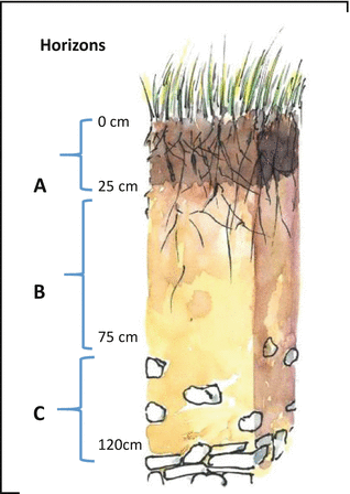
Typical soil profile with different horizons © Ulrich Schmidt
Full size image
Soil texture or grain size distribution (clay: <0.002 mm; silt: 0.002–0.05 mm; sand: 0.05–2 mm), which determines the water-holding capacity and workability of the soil as well as its susceptibility to degradation processes.
The pH, which is a numeric scale used to specify the acidity (pH < 7) or basicity (pH > 7) of the soil.
Soil depth, bulk density and stoniness. These determine the water-holding capacity of the soil, how well it can be treated mechanically, how well plant roots can penetrate it and how much space is available to plant roots for the acquisition of water and nutrients.

Crop production requires the natural resource soil. However, it is directly or indirectly responsible for the largest part of soil degradation processes, such as erosion and compaction. Soil degradation occurs when (a) forests are cleared to make room for agriculture, (b) conversion of land to intensive soil cultivation subjects the organic matter and upper horizons of soil to decomposition and runoff and (c) inappropriate soil cultivation methods lead to compaction and erosion.

Degradation of agricultural soils can be prevented or even reversed by appropriate management methods, but in some cases it requires time spans of decades or centuries for full restoration. Conservation and low-tillage farming, where the tilling of soil is kept to a minimum or avoided altogether, strive to preserve soil fertility. There are a range of measures through which the farmer can maintain soil fertility, including (a) maximizing soil coverage by intercropping, crop rotation optimization and mulching, (b) enhancing soil organic matter supply through intercropping and applying crop residues; (c) reducing soil cultivation intensity and growing perennial crops and (d) avoiding erosion by contour farming, i.e. soil cultivation parallel to slopes.

Soil Erosion

Soil erosion is the physical loss of soil caused by water and wind. Rainfall leads to surface runoff, especially when soil has been cultivated, is not covered by vegetation or is on a steep slope. Wind erosion mainly occurs in semiarid and arid regions. In this process, wind picks up solid particles and carries them away. Erosion is a major process in soil degradation.

1.5 Biological Environment and Agricultural Production

The biological environment (=biotic factors) refers to the natural occurrence of organisms, such as animals, plants, microorganisms, bacteria and viruses, at a specific site. These can all become constraints in crop production and livestock husbandry, for example, through animals eating the crops; weeds competing with crops for nutrients and water; crops becoming infected with fungal, viral or bacterial diseases; or the competition for and lack of fodder of moderate-to-high quality for animal feeding.

At the same time, agricultural production has a strong impact on biodiversity through the use of pesticides, herbicides and fertilizers, increased landscape homogeneity associated with regional and farm-level specialization and habitat losses when natural vegetation is converted to agricultural land (Hilger and Lewandowski 2015; Lambin et al. 2001).

Mixed cropping systems may lead to higher overall product yields than monocultures. However, if the target is the maximization of the yield of one specific crop, the highest area yield is achieved by monoculture, i.e. the cultivation of a single crop or variety in a field at a time. This is because the management system (i.e. crop protection, fertilization, harvesting time) can be best optimized for a homogenous plant community. Any other plants in the field compete with the crop for growth-promoting factors (water, light and nutrients) and are therefore considered weeds that need to be controlled or eradicated in order to avoid a reduction in crop yield. Animals that feed on the crops are also in conflict with agricultural production, except for natural predators of pests (e.g. birds of prey that catch mice) and beneficial insects (e.g. ladybirds than eat aphids), which help to increase agricultural crop productivity.

There are two concepts which are often discussed in the context of agriculture and maintenance of biodiversity: land sharing and sparing. ‘Sharing’ refers to the attempt to integrate as much biodiversity as possible into the agricultural area, generally at the expense of productivity. ‘Sparing’ aims to divide the land into areas used intensively for agriculture and others left natural and uncultivated. There is scientific evidence that the principle of sparing may be more successful in supporting biodiversity than that of sharing.

1.6 Infrastructure and Logistics

Mechanization has greatly enhanced land-use and labour productivity. In modern agricultural production, all processes of soil cultivation, crop establishment, fertilization, crop protection and harvesting are performed mechanically by agricultural machinery specifically optimized for the crop at hand. For this reason, modern agriculture is capital-intensive. In order to secure a reliable and efficient supply chain with low losses, infrastructure and logistics are required for the agricultural production system and storage and transport of the products to the markets. The better the infrastructure and logistic conditions, the lower the supply chain losses. These can reach up to 70% in areas where agricultural infrastructure is poorly developed. The lack of infrastructure (roads, storage facilities) is seen as a major barrier to increasing biomass supply in developing countries. Huge investments would be required to overcome these bottlenecks.

Digitalization is becoming increasingly relevant in contemporary agricultural infrastructure. Modern tractors are equipped with electronic devices, such as GPS (Global Positioning System). In precision farming (see Box 6.4), for example, GPS, electronic sensors and computer programs steer the spatially specific and resource-use-efficient application of agrochemicals.

1.7 Political and Societal Conditions

Agricultural, environmental and market policies have a significant impact on agricultural production in terms of what is produced and how. Examples of market policy impacts are described in Sect. 8.1. Agricultural policy programmes are made by many nations, and so-called common agricultural policies (CAP) determine agricultural policies at EU level. They mainly steer the subsidies provided to farmers and the production volumes of certain agricultural commodities. In the 1990s, European agriculture produced more than the markets could take up without detrimental price effects. Therefore, farmers were obliged to set land aside and and compensated. At that time, 15% of land had to be set aside. Today this land is required for the production of energy and industrial crops, and no more set aside obligations exist. Currently CAP rules determine how agricultural subsidies are coupled to environmental beneficial management measures under the so-called ‘cross-compliance (CC)’, and farmers are obliged to integrate ‘greening areas’ to support biodiversity.

Societal expectations determine how agricultural and environmental policy programmes are framed. For example, in Europe there is little acceptance of genetically modified organisms (GMO; see Sect. 5.1), and the production of GM crops is strictly forbidden.

As has been described above (Sect. 6.1.1), the evolution of farming systems very much depends on social structures, especially how land access is granted and who owns how much land. Also, the educational level of farmers not only determines the success or income of farms, but also whether farmers have the knowledge and willingness to manage their farm sustainably. Finally, the empowerment of farmers is an important condition for shaping a sustainable agriculture for the future.

1.8 Market Conditions

The most important animal-based products globally are cow milk and cattle, pig and chicken meat (see Table 6.2). Rice, wheat and maize are the most important crop-based commodities and are traded globally. Section 8.1 describes how supply and demand steer the agricultural commodity markets and determine market prices.

Table 6.2 Top agricultural products in terms of production value and production quantities, world 2012 (FAOSTAT 2014)

Full size table

There are local, regional and global markets. But it is the demand of those markets that are accessible to farmers that determines what and how much they produce.

Consumer preferences and the consumer’s willingness to buy certain products and to pay a certain price are important market determinants. The willingness of consumers to pay a certain price is especially important for sustainably or ‘better’-produced products. One of the challenges in a bioeconomy is that ecologically more sound production is accompanied by higher production costs. Therefore, bio-based or sustainably produced products are often more expensive than conventional ones. Markets for bio-based products can only develop if consumers are well informed and willing to make a conscious choice for the ‘better’ product.

1.9 Principles of Crop Production

Every crop performs best in specific climatic conditions and can best be grown in either a temperate, subtropical or tropical climate (see also Table 6.1). The climatic profile of a crop is usually determined by the region of its origin (see Fig. 6.7 and also: http://blog.ciat.cgiar.org/origin-of-crops). Breeding (see Sect. 5.1.2) can produce crop varieties that are adapted to specific climatic conditions. A prominent example is maize, whose cultivation area in Europe was extended north by breeding for cold tolerance.

The most important prerequisite for successful crop production is the choice of an appropriate crop and variety for a specific site. This does not only refer to climatic parameters. Crops also have specific demands with regard to soil conditions and biotic (e.g. pests and diseases) and abiotic (e.g. drought, contamination, salinity) stresses. In addition, the appropriate management measures need to be chosen according to the crop and site conditions (see Fig. 6.8). Whereas site conditions are given naturally, crop management is the anthropogenic influence on crop production.

Crop rotation is the temporal sequence of crops on a field. If annual crops (seeding and harvesting in the course of 1 year) are grown, the farmer can choose a new crop every year. Perennial crops are grown on the same field for 3–25 years, depending on the optimal production period of the crop. Intercropping is the integration of a catch crop in between two major crops. Catch crops are often grown to prevent soil runoff (erosion) or nutrient leaching or to provide organic matter to the soil. Crop rotations are generally optimized from an economic viewpoint, i.e. those crops with the highest market value are grown. However, there are biological and physical limits to crop rotation planning. It has to allow enough time for field preparation between the harvesting of one crop and the sowing of the next. Generally, it is not recommended to cultivate the same crop in a field for two or more consecutive years because pests, diseases and weeds often remain in crop residues and soils and can attack the follow-on crop. A change of crop is also necessary due to the depletion of soil nutrients. For this reason, it is recommended to avoid growing the same crop, or crops with similar demands and susceptibility to pests and diseases, in succession.

Soil cultivation is performed to loosen the soil, to incorporate residues, organic and mineral fertilizer, to control weeds and to prepare the soil for sowing or planting. The timing of and technology used for soil cultivation have to be adapted to the demands of the crop and soil conditions. Treating a wet soil and using heavy machinery can have negative impacts on the soil structure (compaction). Ploughing is the most effective soil treatment in terms of soil loosening and weed control. However, to protect soil organic matter and to avoid erosion, less intensive soil cultivation technologies are to be preferred. These, however, can lead to increased weed pressure and weed control demand.

Crops are established via sowing or planting. Sowing is cheaper and easier to mechanize and is the method used for most major crops, such as cereals, maize, sugar, oilseed rape, etc. Some crops have to be planted. Examples are sugar cane, which is established via stem cuttings, and oil palm, established via plantlets. In each case, the soil has to be prepared for planting by loosening it and removing weeds that would hamper crop establishment (soil cultivation).

Fertilization refers to all measures aimed at supplying nutrients to the crop (e.g. application of mineral or organic fertilizer) or improving soil conditions relevant for nutrient uptake (e.g. liming or application of organic substances). The optimal amount of fertilizer is determined according to the expected nutrient demand and withdrawal by the crop. Nitrogen (N) is the nutrient with the strongest yield effect. It is supplied to the soil via mineral or organic fertilizer, N-fixing legumes or atmospheric deposition. In ecological agriculture, N is only supplied via organic fertilizer and biological N fixation (see Box 6.1). In addition, potassium (K), phosphorus (P) and calcium (Ca) are required for optimal crop growth and are generally applied when in shortage. As well as being a plant nutrient, Ca has an influence on soil structure and pH. The so-called crop macronutrients also include magnesium and sulphur (S). These are often combined with PK fertilizer and are only applied when there is an obvious shortage. This also applies to the so-called micronutrients, such as iron (Fe), chloride (Cl), manganese (Mn), zinc (Zn), copper (Cu), boron (B), molybdenum (Mo), cobalt (Co) and nickel (Ni), which are only required in small quantities. Typical fertilizer requirements of major crops, including biomass crops, of temperate regions are shown in Table 6.3.

Table 6.3 List of selected crops with information on water, fertilizer and pesticide demand, parts harvested and constituents utilized

Full size table

Crop protection refers to measures for the suppression or control of weeds, diseases and pests. Weeds compete with crops for all factors affecting growth and reduce crop yield and/or quality. So do pests and diseases, which feed on plant parts or their products of photosynthesis and often reduce the photosynthetically active surface area of plants. Every crop has a range of pests and diseases to which it is susceptible. Diseases can be caused by fungi, bacteria or viruses. If weeds, pests and diseases are not controlled, they can lead to large or total crop losses. There are a number of crop protection measures including mechanical (e.g. weeding) and chemical (herbicides, pesticides (Box 6.2)) methods. In organic agriculture (Box 6.4), no chemical/synthetic crop protection measures are allowed. Instead, biological methods (e.g. natural predators, pheromone traps) are used together with biological pesticides (e.g. extracts from neem tree) and mechanical weed control.

Harvest technology and timing are relevant for the harvest index (proportion of harvested product versus residues) and the quality of the product. Appropriate harvest time and technology avoid pre- and postharvest losses.

Box 6.1: Biological Nitrogen Fixation

Nitrogen (N) is one of the most abundant elements on Earth and occurs predominately in the form of nitrogen gas (N₂) in the atmosphere. There is a specialized group of prokaryotes that can perform biological nitrogen fixation (BNF) using the enzyme nitrogenase to catalyse the conversion of atmospheric nitrogen (N₂) to ammonia (NH₃). Plants can readily use NH₃ as a source of N. These prokaryotes include aquatic organisms (such as cyanobacteria), free-living soil bacteria (such as Azotobacter), bacteria that form associative relationships with plants (such as Azospirillum) and, most importantly, bacteria (such as Rhizobium and Bradyrhizobium) that form symbioses with legumes and other plants (Postgate 1982).

In organic agriculture, BNF is the major N source, and leguminous crops are grown for this purpose. There have been many attempts to associate N-fixing bacteria with crops other than legumes, with the objective of making them independent of external N supply. It is anticipated that BFN will play a major role in the sustainable intensification of agricultural production.

Box 6.2: Pesticides

Pesticide means any substance, or mixture of substances of chemical or biological ingredients, intended for repelling, destroying or controlling any pest or regulating plant growth (FAO and WHO 2014).

Pesticides can have different chemical structures (organic, inorganic, synthetic, biological) and target organisms.

Crop Yields

Crop yields depend on the climatic and management factors depicted in Fig. 6.9. Thus, yield potentials have a climatic/site-specific and a management component. They usually increase with the educational level of farmers and their access to means of production, in particular fertilizer and pesticides. The potential yield on a specific site, which is mainly determined by crop genetics and growth-promoting factors, is generally much higher than the achievable yield (Fig. 6.9). The achievable yield is limited by the availability of nutrients and water and can be improved by yield-increasing measures, such as fertilization and irrigation. The actually harvested yield, however, is normally lower than the achievable yield, because it is reduced by pests and diseases and/or harvest losses. These can partly be overcome through improved crop management and agricultural technology, such as efficient harvesting technology.

The ratio of actual to achievable yield is highest in industrial and lowest in developing countries where farmers have less access to means of agricultural production and are less educated (see Fig. 6.2). For this reason, and also due to climatic differences, it is not possible to provide yield figures for the performance of a crop on every site and for all circumstances. Table 6.4 provides typical, average yields for selected major crops per hectare (ha = 10,000 m²).

Table 6.4 Average yields of selected crops (in dry matter DM) (from KTBL 2015; FNR 2008; FAOSTAT 2014)

Full size table

1.10 Principles of Livestock Production

Global Livestock Population Trends

Global livestock production has a value of at least US$1.4 trillion and employs about 1.3 billion people (Thornton 2010). Livestock has a great significance in the livelihoods of people in the developing world, providing support for 600 million poor smallholder farmers (Thornton 2010). Between 1961 and 2014, the number of animals in the least-developed countries (LDC) increased 2.4-, 7.1- and 6.9-fold for cattle, chicken and pigs, respectively, with major increases in the last two decades. By contrast, in the European Union (EU), livestock populations increased about 1.5-fold between 1961 and the beginning of the 1980s and, since then, have remained more or less stagnant with slight decreases in cattle and slight increases in chicken populations (author’s own calculations; FAOSTAT 2017).

Primary production from livestock has increased in both developing and industrialized countries. In developing regions, this is a result of increasing livestock populations and performance levels (e.g. kg milk or meat/animal), whereas in industrialized countries the growth has almost exclusively been achieved by improving animal performance. There is still a large yield gap between industrialized and developing countries. In 1961, yields of chicken and pig meat per animal were 52% and 92% higher, respectively, in the EU than in the LDC. In 2014, these yields were still 40% and 49% higher, respectively, in the EU than in the LDC. For cattle, the productivity gap between industrialized and developing countries has even increased in the last 50 years. In 1961, milk yields were 9.8-fold higher and meat yields 1.5-fold higher in the EU than in the LDC. In 2014, they were 20- and 2.3-fold higher, respectively (author’s own calculations; FAOSTAT 2017).

Classification of Livestock Production Systems

Livestock production systems vary greatly between different regions of the world, and their development is determined by a combination of socio-economic and environmental factors. Many of these systems are thus the result of a long evolution process and have traditionally been in sustainable equilibrium with their surrounding environments (Steinfeld et al. 2006). Livestock production systems are generally classified based on the following criteria (Seré and Steinfeld 1996; Steinfeld et al. 2006):

Integration with crops
Relation to land
Agroecological zone
Intensity of production
Type of product

In this regard, most livestock production systems are classified into three categories:

Grazing-based systems. In these livestock systems, more than 90% of feed dry mass stems from grassland. Of all the production systems, they cover the largest area: about 26% of the Earth’s ice-free land surface (Steinfeld et al. 2006). This category mainly includes the keeping of ruminants in mobile or sedentary systems. Nomadic and transhumant systems have developed in regions of the world with high inter- or intra-annual variability in precipitation and/or ambient temperatures and thus plant biomass yields of grasslands. Examples include the steppes of Central and East Asia, the semiarid to arid savannahs of Africa and the highlands of Europe, the Middle East, Northern Africa and South America. Sedentary, grazing-based ruminant systems are normally found in regions with higher precipitation, lower climatic variability and higher primary production of grasslands. These include, for instance, ranching systems of North and South America and Australia characterized by large pasture and herd sizes as well as extensive, grazing-based cattle, sheep and goat systems in Europe.
Mixed systems. These are the most important production system worldwide. They typically refer to mixed crop-animal systems, in which livestock by-products such as manure and draught power and crop residues are used as reciprocal inputs and where farmers commonly grow multipurpose crops (e.g. to produce grain for human consumption and stover for animal feed) (Thornton 2010). Two-thirds of the global human population live and within these systems (Thornton 2010). Mixed systems are particularly relevant in developing regions, where they produce about three-quarters each of ruminant milk and meat, 50% of pork and 35% of poultry meat (World Bank 2009).
Landless systems. These systems represent livestock production units in which less than 10% of feed dry mass stems from the unit’s own production (Seré and Steinfeld 1996). They are mainly pig and poultry systems. Globally, 55% of pig meat, 72% of poultry meat and 61% of eggs are produced in these systems (authors’ own calculations; Steinfeld et al. 2006). A minor proportion of beef cattle stocks that are raised in so-called feedlots also belong to this category. Such landless systems are increasingly under pressure due to growing public awareness of environmental and animal welfare issues. In addition, (peri-) urban production units are commonly landless systems. Raising livestock within or in the vicinity of large human settlements provides fresh products to the markets, but also imposes health risks for humans due to the accumulation of animal wastes.

The livestock production systems described above are interrelated, and very often modifications in one system will result in concomitant modifications in another. For example, landless milk production in Kenya depends on grazing-based systems for the replacement of the milking herd (Bebe et al. 2003). Therefore, the size and number of each type of production unit influences the other. Furthermore, human population growth and societal changes put each system under pressure to adjust to evolving market demands, growing urbanization, diminishing availability of traditionally used resources and even increasing public scrutiny. Decreasing access to land and improving access to markets drive the conversion of extensive and mixed systems into more intensive production units, making these systems more efficient in the utilization of inputs to the livestock system. However, some of the systems will not be able to adapt to the new conditions and will collapse (imploding systems) (Fig. 6.10).

Feed Resource Use in Livestock Production Systems

The feed conversion ratio (FCR) is a measure of the amount of feed (e.g. kg dry mass) needed by an animal to produce a unit (e.g. 1 kg) of meat, milk or eggs. It is the inverse of feed conversion efficiency (i.e. the ratio between the product yield and the feed input). Hence, the lower the FCR, the more efficient the conversion of feed energy or nutrients into animal products. The FCR is higher if evaluated at herd level than at the level of an individual producing animal, because the demand for feed biomass of nonproducing animals in the herd is also taken into account. The FCR varies greatly between different livestock products, production systems and regions of the world (Table 6.5). For instance, the FCRs for sheep and goat meat are more than nine times higher than for pig or poultry meat and much higher than for milk. Furthermore, the FCR is higher in grazing-based than mixed and industrial ruminant livestock systems (Herrero et al. 2013) and higher in Sub-Saharan Africa, the Caribbean, Latin America and South Asia than in North America and Europe.

Table 6.5 Feed conversion ratio for the production of milk, meat and eggs by different livestock species (in kg dry feed per kg animal product, evaluated for producing animals) (modified from Smeets et al. 2007; based on Bouwman et al. 2005; Bruinsma 2003)

Full size table

This variation in FCR is mainly determined by the genetic potential of the animals and the intake, digestibility and nutrient concentrations of the available feed, with breeding and health management also playing a role. At low-feed intake level, a major proportion of the energy (and nutrients) ingested by an animal is used for maintenance purposes or is lost via urine and faeces and emission of methane, and only a minor proportion is converted into, for instance, milk or meat. However, with increasing feed intake, the proportion of feed energy (and nutrients) converted into meat, milk or eggs increases (Fig. 6.11; highlighted in green; van Soest 1994). Hence, improving energy and nutrient intakes and thus animal performance will greatly enhance the efficiency of feed resource use in livestock systems.

In line with this, the majority of monogastric livestock worldwide is kept in industrial systems, even in the less-developed countries of South and East Asia, Latin America and Sub-Saharan Africa (see above). Concentrated feeds (i.e. feeds rich in energy and/or protein and generally low in fibre, such as cereal grains and their by-products) as well as soybean and fish meal as high-quality protein sources commonly account for more than 80% of their diet (on a dry matter basis; Seré and Steinfeld 1996; Herrero et al. 2013). The high digestibility of these feeds promotes intake and animal growth rates. Consequently, the FCR in pig and poultry systems are much lower than in ruminant livestock (except dairy production) and are very similar across the various regions of the world.

By contrast, ruminant feeding is much more diverse, and their diets comprise (on a dry matter basis) at least 50% roughage (i.e. bulky feeds with generally higher fibre concentrations and lower digestibility than concentrate feeds) with a few exceptions such as beef cattle finishing in feedlots. Moreover, the slower maturation and longer reproductive cycles of ruminants, as compared to pigs and poultry, result in higher proportions of nonproducing animals within the herds. Consequently, the FCR at both the animal and system level is higher in ruminant than in monogastric livestock. The FCR in milk production is lowest. Because milk contains about 85% water, its nutrient and energy density is very low compared to other animal-derived food products. While most ruminant livestock in industrialized countries is kept in mixed systems (Seré and Steinfeld 1996) where feeding is based on cultivated forage and concentrate feeds, animals in other regions of the world commonly graze on (semi-)natural grasslands or are fed crop residues, and use of concentrate feeds is lower. These differences in diet composition and hence performance of animals are responsible for the differences in the FCR of ruminant products between the various production systems and regions of the world.

Box 6.3: Feed Conversion Ratio (FCR)

Common approaches to evaluating the FCR and ecological footprints of livestock systems do not differentiate between the types of plant biomass used as feed. For instance, the use of feed resources inedible for humans, such as roughage and crop residues, may reduce competition with plant biomass as food or feed. When expressed as the amount of energy and protein from human-edible feeds per unit of animal product, differences in FCR between livestock products become much smaller, because ruminant diets typically contain lower proportions of feeds suitable for human consumption. In some cases, the FCR is even lower for the production of beef than for pork, poultry meat and eggs (Wilkinson 2011). Similarly, these approaches only focus on either milk, meat or eggs as primary products and do not (adequately) account for other outputs or services provided by livestock. For instance, animal manure is an important source of nutrients for the maintenance of soil fertility in crop production, in particular in mixed farming systems of Sub-Saharan Africa, Latin America and South and East Asia. Neglecting this additional output overestimates the actual FCR in mixed systems. Also, calves born in dairy cattle systems are also raised to produce meat. Correcting for the greenhouse gases emitted during the production of the same amount of meat in specialized beef cattle systems considerably reduces the carbon footprint of cow milk (Flysjo et al. 2012) and diminishes the differences between various production systems.

As the vast majority of expenses in livestock husbandry comes from the provision of animal feed, the FCR greatly determines the profitability of livestock farming. Moreover, the FCR is a key determinant of the demand for natural resources and the emissions of environmental pollutants in livestock systems. For instance, about 98% of the water needed to produce animal products (i.e. water footprint) is related to the production, processing, transport and storage of feed for livestock, whereas only 1% each is needed as drinking or service water (Mekonnen and Hoekstra 2010). Accordingly, the water footprints of beef, mutton and goat meat are higher than of pig and poultry meat and are even higher in grazing-based than in mixed or industrial ruminant systems, in particular those of Europe and North America characterized by a lower FCR. There are similar differences in the carbon footprint of animal products (Herrero et al. 2013). Hence, any improvements in the FCR will greatly contribute to increasing profitability and reducing environmental emissions and (natural) resource use in livestock farming.

1.11 Towards Sustainable (Intensification of) Agriculture

In the bioeconomy, agriculture needs to be performed sustainably. This requires a definition and characterization of sustainable agriculture. One approach is to categorize farming systems according to their management concepts (see Fig. 6.12). Industrial farming aims to maximize economic benefit through a high level of mechanization and the application of synthetic pesticides and fertilizers for crop production and through the utilization of specialized breeds and intense feeding, health and reproductive management for animal production. Integrated farming uses both synthetic and biological means of nutrient supply and pest control, but applies input and management measures at levels considered economically justified and that reduce or minimize ecological and health risks. Additionally, integrated farming makes use of naturally occurring strengths in plants and animals used for production purposes, like resistance to drought in certain crops or tolerance to diseases and parasites in certain animal breeds. The conservation of natural resources, including genetic resources, is at the focus of both organic farming and conservation farming. In organic farming, no synthetic fertilizers, pesticides or feed supplements are allowed. Conservation farming mainly focuses on agronomical practices that enhance soil conservation via, e.g. cover crops or incorporation of crop residues into the soil; here there might be a conflict with livestock in mixed production systems because livestock will compete for crop residues as feed and may compromise the objectives of conservation agriculture. Finally, precision farming strives to minimize agricultural inputs by applying spatially specific management to crops and accurate and timely feeding to animals using modern agricultural technologies including digitalization (see Box 6.4). All these farming concepts apply management rules to define and operationalize sustainable agricultural management.

Box 6.4: Farming Concepts with a Clear Definition (Rather Than a Conceptual Approach)

Good Agricultural Practice (GAP)

‘Good Agricultural Practice (GAP), for instance in the use of pesticides, includes the officially recommended or nationally authorized uses of pesticides under actual conditions necessary for effective and reliable pest control. It encompasses a range of levels of pesticide applications up to the highest authorized use, applied in a manner which leaves a residue which is the smallest amount practicable’ (FAO and WHO 2014). With respect to, for instance, health management in livestock farming, GAP includes the prevention of entry of diseases onto the farm, an effective health management (e.g. record keeping, animal identification and monitoring) and the use of chemicals and medicines as described (IDF and FAO 2004).

In the EU, ‘good farming practice’ (GFP) is used synonymously with GAP. National codes of GFP constitute minimum standards for farm management and serve as a precondition for payments to farmers in the context of ‘cross-compliance’. Cross-compliance is the attachment of environmental conditions to agricultural support payments (Baldock and Mitchell 1995) and is an obligatory element of the Common Agricultural Policy (CAP). In the EU, cross-compliance as well as GAP rules are generally laid down in laws or legal guidelines.

Integrated Farming

Integrated farming seeks to optimize the management and inputs of agricultural production in a responsible way, through the holistic consideration of economic, ecological and social aspects. This approach aims at minimizing the input of agrochemicals and medicines to an economical optimum and includes ecologically sound management practices as much as possible. As one example, ‘Integrated Pest Management (IPM) means the careful consideration of all available pest control techniques and subsequent integration of appropriate measures that discourage the development of pest populations and keep pesticides and other interventions to levels that are economically justified and reduce or minimize risks to human and animal health and/or the environment. IPM emphasizes the growth of a healthy crop with the least possible disruption to agro-ecosystems and encourages natural pest control mechanisms’ (FAO and WHO 2014). Moreover, the close linkage of crop and livestock components in agroecosystems allows for efficient recycling of agricultural by-products or wastes, thereby reducing the reliance on external inputs such as fertilizers or animal feeds.

Organic Farming

‘Organic Agriculture is a production system that sustains the health of soils, ecosystems and people. It relies on ecological processes, biodiversity and cycles adapted to local conditions, rather than the use of inputs with adverse effects. Organic Agriculture combines tradition, innovation and science to benefit the shared environment and promote fair relationships and a good quality of life for all involved’ (IFOAM 2005). There are several variants of organic agriculture, including livestock organic production. All of them forbid the use of synthetic pesticides and fertilizers in crop production. Crop nutrient demands and crop health are managed through biological methods of N fixation, crop rotation and the application of organic fertilizer, especially animal manure. Regarding livestock, organic production fosters the welfare of animals, and it restricts the use of synthetic feed supplements to those conditions where the welfare of the animal might be compromised by a serious deficiency. Similarly, organic livestock production focuses on disease prevention, and it prohibits the use of antibiotics, unless any other option is available to stop the animal from suffering.

Precision Farming

Precision farming is a management approach based on the spatially specific and targeted management of agricultural land and fields. It makes use of modern agricultural production technology and is often computer-aided. In crop farming, the objective of precision farming is to take account of small-scale differences in management demand within fields. Sensors that assess the nutritional status and health of crops support their spatially differentiated management. Similarly, precision farming in livestock production aims at (continuous) monitoring of, for instance, the nutrition, performance, health and reproductive status of (individual or small groups of) animals in real-time. Such information helps farmers to make appropriate decisions in animal, feed or grazing management to optimize production, health and welfare of animals but also to increase efficiency of natural resource use in and reduce environmental impact of livestock farming.

Conservation Farming

‘Conservation Agriculture (CA) is an approach to managing agroecosystems for improved and sustained productivity, increased profits and food security while preserving and enhancing the resource base and the environment. CA is characterized by three linked principles, namely:

Continuous minimum mechanical soil disturbance.
Permanent organic soil cover.
Diversification of crop species grown in sequences and/or associations’ (FAO 2017a).

In a future bioeconomy, agriculture will need to make combined use of all available knowledge and technology that can help increase productivity while, at the same time, reducing the negative environmental impacts of agricultural production. This vision is also described as ‘sustainable intensification’ (see Box 6.4).

Box 6.5: Sustainable Agricultural Intensification

The Royal Society (2009) defined sustainable intensification as a form of agricultural production (both crop and livestock farming) whereby ‘yields are increased without adverse environmental impact and without the cultivation of more land’. More recently, Pretty et al. (2011) extended this definition of sustainable agricultural intensification to ‘producing more output from the same area of land while reducing the negative environmental impacts and at the same time, increasing contributions to natural capital and the flow of environmental services’.

Box 6.6: Sustainable Intensification of Livestock Production

Examples of India and Kenya show that small changes in feeding practices like balancing diet with the same feed ingredients, feeding small additional amounts of concentrate and introducing cooling systems can greatly increase yields and total animal production and the sustainability of the production systems (Garg et al. 2013; Upton 2000).

There is evidence that the nutrient-use efficiency increases, while the intensity of methane emissions (g/kg milk) decreases by feeding nutritionally balanced rations designed from locally available resources in smallholders of cattle and buffaloes (Garg et al. 2013).

Even though challenging, larger improvements can be made in those production systems where the animal is still far from reaching its genetic potential for production, like those typically found in tropical and in developing regions.

Other intensification option is the more systematic use of agricultural or industrial by-products. However, one main problem of these materials is the unknown content of nutrients, therefore, a characterization of the available resources per region and their feeding value for each species may help to introduce them as ingredients in animals’ diets. In this regard, even at the production units with high levels of intensification, advances towards sustainability can be made. In recent years the inclusion of citrus by-product from the juice industry has been regularly practised in dairy cattle diets.

Moreover, later examples have shown that small proportions of crop residues like wheat straw and corn stover—as source of physically effective fibre—can be included in diets of high-yielding dairy cows without negative impacts on yields (Eastridge et al. 2017). Such by-products have been traditionally assumed not to be suitable for diets of high-yielding animals and have been rather associated in mixed systems with less productive animals.

The use of local forages as source of protein can also aid to the sustainable intensification of production systems. However, for a farmer to adopt any management practice, this has to fit into the farmer’s daily routine or only minimally alter it; additionally, it should allow the farmer to afford it.

In order to define and describe the goals of sustainable agriculture, relevant criteria need to be established. Discussions in various international, multi-stakeholder roundtables have led to a set of internationally accepted criteria being compiled. The general criteria of the sustainability standards elaborated by these roundtables are shown in Table 6.6.

Table 6.6 Summary of criteria for sustainable agricultural production and biomass supply, compiled from the sustainability studies of the Roundtable on Sustainable Palm Oil (RSPO), the Round Table on Responsible Soy (RTRS), Bonsucro and the Roundtable on Sustainable Biomaterials (RSB) (from Lewandowski 2015)

Full size table

However, even if we manage to set the criteria for sustainable agriculture, the aspiration of ‘absolute’ sustainability appears inoperable. This is because the manifold trade-offs between sustainability goals and conflicting stakeholder perceptions of sustainability render the simultaneous fulfilment of all sustainability criteria shown in Table 6.6 impossible. Therefore, the concept of sustainable agricultural intensification will need to strive for the best possible compromise between productivity increase and natural resource conservation.

There are many options for increasing agricultural productivity. Figure 6.13 shows the numerous technical approaches that can contribute to this goal. These include breeding of efficient crop varieties and animal breeds; development of efficient, site-specific crop and livestock management and land-use systems; development of specific feeding strategies for an animal type and region (see Box 6.6); logistic optimization; and exploration of new biomass resource options, such as algae and biomass from permanent grasslands.

The largest potential for maximizing yields through improved cropping and livestock systems is seen in approaches targeted at closing the yield gap between achievable and actually harvested yields. In many regions of Africa, Latin America and Eastern Europe, this gap averages up to 55% (FAO 2002). The problem is often not the biophysical suitability of the site, ‘site x crop combination’ or production potential of livestock animals but insufficient agronomical practices and policy support (Yengoh and Ardo 2014). However, to avoid the intensification of agricultural production necessary to exploit the yield gap becoming, or being perceived as, ecologically ‘unsustainable’, concepts for ‘sustainable intensification’ need to be elaborated. In addition, advanced agricultural technologies, such as precision farming (Box 6.4), that can improve productivity without negative ecological impacts, need to be further developed.

The provision of technical solutions for the improvement of cropping and livestock systems alone will, however, not be sufficient to mobilize the sustainable biomass supply. Farmers must also be willing to adopt these solutions and see an advantage in their application (Nhamo et al. 2014). Also, farmers must be able to afford the agricultural inputs required and be in a position to apply them. This calls for support through credit programmes and access for farmers to markets and training programmes (Nhamo et al. 2014).

Agriculture and Greenhouse Gas (GHG) Emissions

Agriculture also needs to contribute to climate change mitigation via a reduction of greenhouse gas (GHG) emissions. The main GHGs are carbon dioxide (CO₂), methane (CH₄) and nitrous oxide (N₂O). Presently, global agriculture emits about 5.1–6.1 Gt CO_2equivalents of GHG a year (Smith et al. 2007). CO₂ is mainly released from microbial decay or burning of plant litter and soil organic matter and also comes from the use of fossil resources in agricultural production. CH₄ is mainly produced from fermentative digestion by ruminant livestock, from the storing of manure and from rice grown in flooded conditions (Mosier et al. 1998). N₂O comes from nitrification and denitrification of N in soils and manures, or from N volatilization, leaching and runoff, and its emission is enhanced with higher levels of N fertilization (for soils) or high levels of N feeding (for animals) (IPCC 2006).

The global technical potential for GHG mitigation in agriculture is estimated to be in the range of 4.5–6.0 Gt CO_2equivalents/year if no economic or other barriers are considered (Smith et al. 2007). In general, GHG emissions can be reduced by increasing plant and animal productivity (i.e. unit of final product per unit of area or per animal) and by more efficiently managing inputs into the system (e.g. applying the appropriate amount of fertilizer needed for a particular crop under the soil/climatic conditions, closed nutrient cycling). Other options include land management that increases soil carbon sequestration (e.g. agroforestry), improving diet quality to reduce enteric CH₄ formation, soil management that enhances the oxidation of CH₄ in paddy fields and manure management that minimizes N₂O formation. Finally, also the use of bioenergy is a mitigation option (see Fig. 6.14; for details on agricultural GHG mitigation options, see Smith et al. 2007).

Review Questions

What are the main determinants for the kind of agricultural production performed?
What are the management options for improving productivity in crop and animal production?
What is sustainable agriculture and sustainable intensification?
How can negative environmental impacts of agricultural production be minimized?

References

Ahmed F, Fanning K, Netzel M et al (2014) Profiling of carotenoids and antioxidant capacity of microalgae from subtropical coastal and brackish waters. Food Chem 165:300–306. https://doi.org/10.1016/j.foodchem.2014.05.107
Ahmed F, Zhou W, Schenk PM (2015) Profiling of carotenoids and antioxidant capacity of microalgae from subtropical coastal and brackish waters. Algal Res 10:210–217. https://doi.org/10.1016/j.algal.2015.05.013
Albion RG (1926) Forests and sea power: the timber problem of the royal navy, 1652–1862. Revised edition (December 1999) edn. US Naval Institute Press
Anderson JL (2012) Mahogany – the costs of luxury in early America. Harvard University Press, Cambridge
Arbeitsgemeinschaft Forsteinrichtung/Arbeitskreis für Standortskartierung (1985) Forstliche Wuchsgebiete und Wuchsbezirke in der Bundesrepublik Deutschland. Landwirtschaftsverlag, Münster-Hiltrup
Baldock D, Mitchell K (1995) Cross-compliance within the common agricultural policy: a review of options for landscape and nature conservation. Institute of European Environmental Policy, Brussels
Batista AP, Gouveia L, Bandarra NM et al (2013) Comparison of microalgal biomass profiles as novel functional ingredient for food products. Algal Res 2:164–173. https://doi.org/10.1016/j.algal.2013.01.004
Bebe BO, Udo HMJ et al (2003) Smallholder dairy systems in the Kenya highlands: cattle population dynamics under increasing intensification. Livest Prod Sci 82(2-3):211–221. https://doi.org/10.1016/S0301-6226(03)00013-7
Becker EW (2007) Micro-algae as a source of protein. Biotechnol Adv 25:207–210. https://doi.org/10.1016/j.biotechadv.2006.11.002
Bergmann P et al (2013) Disposable flat panel airlift photobioreactors. Chem Ing Tech. 85:202–205. https://doi.org/10.1002/cite.201200132
BMEL (2017) Bundesministerium für Ernährung und Landwirtschaft. http://www.bmel-statistik.de/
Bouwman AF, Van Der Hoek KW et al (2005) Exploring changes in world ruminant production systems. Agric Syst 84(2):121–153. https://doi.org/10.1016/j.agsy.2004.05.006
Brennan L, Owende P (2010) Biofuels from microalgae—a review of technologies for production, processing, and extractions of biofuels and co-products. Renew Sustain Energy Rev 14:557–577. https://doi.org/10.1016/j.rser.2009.10.009
Bruinsma J (2003) World agriculture: towards 2015/2030. An FAO perspective. Food and Agriculture Organization (FAO). https://doi.org/10.1016/S0264-8377(03)00047-4
Busing RT, Fujimori T (2005) Biomass, production and woody detritus in an old coast redwood (Sequoia sempervirens) forest. Plant Ecol 177(2):177–188
Byelashov OA, Griffin ME (2014) Fish in: fish out: perception of sustainability and contribution to public health. Fisheries 39(11):531–535. https://doi.org/10.1080/03632415.2014.967765
Cerón-García MC, Fernández-Sevilla JM, Sánchez-Mirón A et al (2013) Mixotrophic growth of Phaeodactylum tricornutum on fructose and glycerol in fed-batch and semi-continuous modes. Bioresour Technol 147:569–576. https://doi.org/10.1016/j.biortech.2013.08.092
Chini Zittelli G, Lavista F, Bastianini A et al (1999) Production of eicosapentaenoic acid by Nannochloropsis sp. cultures in outdoor tubular photobioreactors. J Biotechnol 70:299–312. https://doi.org/10.1016/s0168-1656(99)00082-6
Das P, Thaher MI, Hakim MAQM et al (2015) Sustainable production of toxin free marine microalgae biomass as fish feed in large scale open system in the Qatari desert. Bioresour Technol 192:97–104. https://doi.org/10.1016/j.biortech.2015.05.019
Dauber J, Brown C et al (2012) Bioenergy from “surplus” land: environmental and socio-economic implications. BioRisk. https://doi.org/10.3897/biorisk.7.3036
Davis SC, Hay W, Pierce J (2014) Biomass in the energy industry: an introduction. Published by BP p.l.c.
De Silva SS (1995) Supplementary feeding in semi-intensive aquaculture systems. In: New MB, Tacon AGJ, Csavas I (eds) Farm-made aquafeeds. FAO Fisheries Technical Paper 343. FAO, Rome, pp 24–60
Dixon J, Gulliver A, Gibbon D (2001) Farming systems and poverty: improving farmers’ livelihoods in a changing world. FAO/World Bank, Rome/Washington, DC. https://doi.org/10.1017/S0014479702211059
DJV (2017) DJV-Handbuch Jagd. DJV-Service GmbH, Bonn
Dornburg V, van Vuuren D et al (2010) Bioenergy revisited: key factors in global potentials of bioenergy. Energy Environ Sci. https://doi.org/10.1039/b922422j
Eastridge ML, Starkey RA et al (2017) Dairy cows fed equivalent concentrations of forage neutral detergent fiber from corn silage, alfalfa hay, wheat straw, and corn stover had similar milk yield and total tract digestibility. Anim Feed Sci Technol 225:81–86
Edwards P, Pullin RSV, Gartner JA (1988) Research and education for the development of integrated crop-livestock-fish farming systems in the tropics. International Center for Living Aquatic Resources Management, Manila
FAO (1982) Classification and definitions of forest products. Food and Agriculture Organization of the United Nations, Rome, p 250
FAO (1997) Aquaculture development. FAO Technical Guidelines for Responsible Fisheries 5. FAO, Rome
FAO (2000) On the definition of forest and forest change. Food and Agriculture Organization of the United Nations, Rome, p 15
FAO (2002) World agriculture: towards 2015/2030. An FAO perspective, Food Agricultural Organisation. Earthscan Publications Ltd, London, p 106
FAO (2010) Global forest resources assessment 2010. Food and Agriculture Organization of the United Nations, Rome
FAO (2014) The state of world fisheries and aquaculture 2014. Opportunities and Challenges. Rome
FAO (2015a) Global forest resources assessment 2015. Food and Agriculture Organization of the United Nations, Rome
FAO (2015b) Fisheries and Aquaculture Department, Statistics and Information Service FishStatJ: Universal software for fishery statistical time series
FAO (2016) The state of world fisheries and aquaculture 2016. Contributing to food security and nutrition for all. Rome
FAO (2017a) What is conservation agriculture? http://www.fao.org/ag/ca/1a.html. Accessed 8 Jan 2017
FAO (2017b) FAOSTAT-forestry database. Food and Agriculture Organization of the United Nations, Rome
FAO (Food and Agricultural Organization of the United Nations) and WHO (World Health Organization) (2014) The international code of conduct on pesticide management. Rome, Italy. E-ISBN: 978-92-5-108549-3. http://www.fao.org/fileadmin/templates/agphome/documents/Pests_Pesticides/Code/CODE_2014Sep_EN. Accessed 8 Jan 2017
FAO GeoNetwork (2017a) http://www.fao.org/geonetwork/srv/en/main.home. Accessed 23 Feb 2017
FAO GeoNetwork (2017b) FAO GeoNetwork. http://www.fao.org/geonetwork/srv/en/main.home. Accessed 23 Feb 2017
FAOSTAT (2014) Food and agriculture organization of the United States – Statistics Division. http://faostat.fao.org/
FAOSTAT (2017) Statistical Database. Rome. www.fao.org/faostat/en/#data/QA
Flysjo A, Cederberg C et al (2012) The interaction between milk and beef production and emissions from land use change – critical considerations in life cycle assessment and carbon footprint studies of milk. J Clean Prod. https://doi.org/10.1016/j.jclepro.2011.11.046
FNR (2008) Studie zur Markt- und Konkurrenzsituation bei Naturfasern und Naturfaserwerkstoffen (Deutschland und EU). In: Gülzower Fachgespräche 26, Fachagentur Nachwachsende Rohstoffe e.V., Gülzow
Francavilla M, Trotta P, Luque R (2010) Phytosterols from Dunaliella tertiolecta and Dunaliella salina: a potentially novel industrial application. Bioresour Technol 101:4144–4150. https://doi.org/10.1016/j.biortech.2009.12.139
Frankfurt a.M. (2017) Stadtwald. Stadt Frankfurt am Main. https://www.frankfurt.de/sixcms/detail.php?id=2800&_ffmpar%5b_id_inhalt%5d=101676. Accessed 10 Jul 2017
Garg MR, Sherasia PL et al (2013) Effects of feeding nutritionally balanced rations on animal productivity, feed conversion efficiency, feed nitrogen use efficiency, rumen microbial protein supply, parasitic load, immunity and enteric methane emissions of milking animals under field conditions. Anim Feed Sci Technol 179(1):24–35
Gille A, Trautmann A, Posten C et al (2016) Bioaccessibility of carotenoids from Chlorella vulgaris and Chlamydomonas reinhardtii. Int J Food Sci Nutr 67:507–513. https://doi.org/10.1080/09637486.2016.1181158
Giri C, Ochieng E, Tieszen LL et al (2010) Status and distribution of mangrove forests of the world using earth observation satellite data. Glob Ecol Biogeogr: J Macroecol 20(1):154–159
Gliessman SR (2015) Agroecology: the ecology of sustainable food systems. CRC Press, Boca Raton
Good R (1947) The geography of the flowering plants. Longmans, Green, London
Granado F, Olmedilla B, Blanco I (2003) Nutritional and clinical relevance of lutein in human health. Br J Nutr 90(3):487–502. https://doi.org/10.1079/BJN2003927
Guo Z, Zhang Y, Deegen P et al (2006) Economic analyses of rubber and tea plantations and rubber-tea intercropping in Hainan, China. Agrofor Syst 66(2):117–127. https://doi.org/10.1007/s10457-005-4676-2
Hardy RW (2010) Utilization of plant proteins in fish diets: effects of global demand and supplies of fishmeal. Aquacult Res 41(5):770–776. https://doi.org/10.1111/j.1365-2109.2009.02349.x
Harrison RP (1992) Forests – the shadow of civilization. The University of Chicago Press, Chicago
Harun R (2010) Bioprocess engineering of microalgae to produce a variety of consumer products. Renew Sustain Energy Rev 14:1037–1047. https://doi.org/10.1016/j.rser.2009.11.004
Hernández C, Olvera-Novoa MA, Hardy RW et al (2010) Complete replacement of fish meal by porcine and poultry by-product meals in practical diets for fingerling Nile tilapia Oreochromis niloticus: digestibility and growth performance. Aquacult Nutr 16(1):44–53. https://doi.org/10.1111/j.1365-2095.2008.00639.x
Herrero M, Havlik P et al (2013) Biomass use, production, feed efficiencies, and greenhouse gas emissions from global livestock systems. Proc Natl Acad Sci. https://doi.org/10.1073/pnas.1308149110
Hilger T, Lewandowski I (2015) Seeds of change—plant genetic resources and people’s livelihoods. In: Pilipavičius V (ed) Agroecology. IN TECH, Rijeka
Hoogwijk M, Faaij A, Eickhout B et al (2005) Potential of biomass energy out to 2100, for four IPCC SRES land-use scenarios. Biomass Bioenergy. https://doi.org/10.1016/j.biombioe.2005.05.002
Hummer KE, Hancock JF (2015) Vavilovian centers of plant diversity: implications and impacts. HortScience 50:780–783
IFAD (2013) Smallholders, food security and the environment. Human behavior and environment
IFOAM (International Federation of Organic Agriculture Movement) (2005) http://www.ifoam.bio/en/organic-landmarks/definition-organic-agriculture. Accessed 8 Jan 2017
Imhoff ML, Bounoua L, Ricketts T et al (2004) Global patterns in human consumption of net primary production. Nature. https://doi.org/10.1038/nature02619
International Dairy Federation (IDF) and Food and Agriculture Organization (FAO) (2004) Guide to good dairy farming practice. Rome. ISBN: 92-5-105094-5
IPCC (2006) 2006 Guidelines for national greenhouse gas inventories. In: Eggleston HS, Buendia L, Miwa K, Ngara T, Tanabe K (eds) Prepared by the national greenhouse gas inventories programme. IGES, Japan
Jacobs MR (1955) Growth habits of the eucalypts. Forestry and Timber Bureau, Canberra
Kaushik S, Troell M (2010) Taking the fish-in fish-out ratio: a step further…. Aquacult Eur 35:15–17
Khoury CK, Achicanoy HA et al (2016) Origins of food crops connect countries worldwide. Proc R Soc B: Biol Sci. https://doi.org/10.1098/rspb.2016.0792
Knigge W, Schulz H (1966) Grundriss der Forstbenutzung. Paul Parey, Hamburg
Kost C, Mayer JN, Thomsen J et al (2013) Levelized Cost of Electricity Renewable Energy Technologies. Fraunhofer Institute for Solar Energy Systems ISE, Stuttgart
Krienitz L, Wirth M (2006) The high content of polyunsaturated fatty acids in Nannochloropsis limnetica (Eustigmatophyceae) and its implication for food web interactions, freshwater aquaculture and biotechnology. Limnologica 36:204–210. https://doi.org/10.1016/j.limno.2006.05.002
Krutilla, JV, Fisher AC (1975) The economics of natural environments; studies in the valuation of commodity and amenity resources. The Johns Hopkins University Press, Baltimore (quoted in Perman R, Yue M et al (2011) Natural Resource and Environmental Economics, 4th edn. Pearson, Harlow, p 395ff)
KTBL (2015) KTBL-Taschenbuch Landwirtschaft Kuratorium für Technik und Bauwesen in der Landwirtschaft e.V. Kuratorium für Technik und Bauwesen in der Landwirtschaft, Darmstadt
Lambin EF, Turner BL et al (2001) The causes of land use and land cover change: moving beyond the myths. Glob Environ Change 11(4):261–269
Lamprecht H (1989) Silviculture in the Tropics. Deutsche Gesellschaft für Technische Zusammenarbeit (GTZ) GmbH, Eschborn
Lewandowski I (2015) Securing a sustainable biomass supply in a growing bioeconomy. Glob Food Sec. https://doi.org/10.1016/j.gfs.2015.10.001
Liau BC, Shen CT, Liang FP et al (2010) Supercritical fluids extraction and anti-solvent purification of carotenoids from microalgae and associated bioactivity. J Supercrit Fluids 55:169–175. https://doi.org/10.1016/j.supflu.2010.07.002
Lowder SK, Skoet J, Raney T (2016) The number, size, and distribution of farms, smallholder farms, and family farms worldwide. World Dev. https://doi.org/10.1016/j.worlddev.2015.10.041
Macías-Sánchez MD, Mantell C, Rodríguez et al (2007) Supercritical fluid extraction of carotenoids and chlorophyll a from Synechococcus sp. J Supercrit Fluids 39:323–329. https://doi.org/10.1016/j.supflu.2006.03.008
Martin K, Sauerborn J (2013) Agroecology. Springer, Amsterdam
Martins JG (2009) EPA but not DHA appears to be responsible for the efficacy of omega-3 long chain polyunsaturated fatty acid supplementation in depression: evidence from a meta-analysis of randomized controlled trials. J Am Coll Nutr 28(5):525–542. https://doi.org/10.1080/07315724.2009.10719785
Mata TM, Martins AA, Caetano NS (2010) Microalgae for biodiesel production and other applications: a review. Renew Sustain Energy Rev 14:217–232. https://doi.org/10.1016/j.rser.2009.07.020
Meiser A, Schmid-Staiger U, Trösch W (2004) Optimization of eicosapentaenoic acid production by Phaeodactylum tricornutum in the flat panel airlift (FPA) reactor. J Appl Phycol 16:215–225. https://doi.org/10.1023/B:JAPH.0000048507.95878.b5
Mekonnen MM, Hoekstra AY (2010) The green, blue and grey water footprint of farm animals and animal products. UNESCO-IHE Institute for Water Education. https://doi.org/10.5194/hess-15-1577-2011
Mendes RL, Nobre BP, Cardoso MT et al (2003) Supercritical carbon dioxide extraction of compounds with pharmaceutical importance from microalgae. Inorg Chim Acta 356:328–334. https://doi.org/10.1016/S0020-1693(03)00363-3
Mitchell HH, Hamilton TS et al (1932) The effect of the amount of feed consumed by cattle on the utilization of its energy content. J Agric Res 45:163
Morales-Sánchez D, Tinoco-Valencia R, Caro-Bermúdez MA et al (2014) Culturing Neochloris oleoabundans microalga in a nitrogen-limited, heterotrophic fed-batch system to enhance lipid and carbohydrate accumulation. Algal Res 5:61–69. https://doi.org/10.1016/j.algal.2014.05.006
Mosier A, Kroeze C et al (1998) Closing the global N2O budget: nitrous oxide emissions through the agricultural nitrogen cycle. OECD/IPCC/IEA phase II development of IPCC guidelines for national greenhouse gas inventory methodology. Nutr Cycl Agroecosyst 52:225
Mulders KJM, Janssen JH, Martens DE et al (2014) Effect of biomass concentration on secondary carotenoids and triacylglycerol (TAG) accumulation in nitrogen-depleted Chlorella zofingiensis. Algal Res 6:8–16. https://doi.org/10.1016/j.algal.2014.08.006
Münkel R, Schmid-Staiger U, Werner A et al (2013) Optimization of outdoor cultivation in flat panel airlift reactors for lipid production by Chlorella vulgaris. Biotechnol Bioeng 110:2882–2893
Nachtergaele F, Petri M (2008) Mapping land use systems at global and regional scales for land degradation assessment analysis. LADA Technical Report
Neori A, Nobre AM (2012) Relationship between trophic level and economics in aquaculture. Aquacult Econ Manage 16:40–67
Nhamo N, Rodenburg J et al (2014) Narrowing the rice yield gap in east and Southern Africa: using and adapting existing technologies. Agric Syst. https://doi.org/10.1016/j.agsy.2014.08.003
Norsker NH, Barbosa MJ, Vermuë MH et al (2011) Microalgal production—a close look at the economics. Biotechnol Adv 29:24–27. https://doi.org/10.1016/j.biotechadv.2010.08.005
Pal D, Khozin-Goldberg I, Cohen Z et al (2011) The effect of light, salinity, and nitrogen availability on lipid production by Nannochloropsis sp. Appl Microbiol Biotechnol 90:1429–1441. https://doi.org/10.1007/s00253-011-3170-1
Parniakov O, Barba FJ, Grimi N et al (2015) Pulsed electric field assisted extraction of nutritionally valuable compounds from microalgae Nannochloropsis spp. using the binary mixture of organic solvents and water. Innov Food Sci Emerg Technol 27:79–85. https://doi.org/10.1016/j.ifset.2014.11.002
Pasquet V, Chérouvrier JR, Farhat F et al (2011) Study on the microalgal pigments extraction process: Performance of microwave assisted extraction. Process Biochem 46:59–67. https://doi.org/10.1016/j.procbio.2010.07.009
Pauly D (2009) Beyond duplicity and ignorance in global fisheries. Sci Mar 73(2):215–224
Perez-Garcia O, Escalante FME, Bashan LE et al (2011) Heterotrophic cultures of microalgae: metabolism and potential products. Water Res 45:11–36. https://doi.org/10.1016/j.watres.2010.08.037
Perman R, Yue M, Common M et al (2011) Natural resource and environmental economics, 4th edn. Pearson, Harlow
Pieber S, Schober S, Mittelbach M (2012) Pressurized fluid extraction of polyunsaturated fatty acids from the microalga Nannochloropsis oculata. Biomass Bioenergy 47:474–482. https://doi.org/10.1016/j.biombioe.2012.10.019
Piotrowski S, Essel R et al (2015) Nachhaltig nutzbare Potenziale für Biokraftstoffe in Nutzungskonkurrenz zur Lebens-und Futtermittelproduktion, Bioenergie sowie zur stofflichen Nutzung in Deutschland, Europa und der Welt. http://bio-based.eu/downloads/nachhaltig-nutzbare-potenziale-fuer-biokraftstoffe-in-nutzungskonkurrenz-zur-lebens-und-futtermittelproduktion-bioenergie-sowie-zur-stofflichen-nutzung-in-deutschland-europa-und-der-welt/
Plaza M, Santoyo S, Jaime L (2012) Comprehensive characterization of the functional activities of pressurized liquid and ultrasound-assisted extracts from Chlorella vulgaris. LWT – Food Sci Technol 46:245–253. https://doi.org/10.1016/j.lwt.2011.09.024
Posten C, Feng Chen S (eds) (2016) Microalgae biotechnology, Advances in biochemical engineering/biotechnology. Springer International Publishing, Cham
Postgate JR (1982) The fundamentals of nitrogen fixation. Cambridge University Press, Cambridge
Prein M (2002) Integration of aquaculture into crop-animal systems in Asia. Agricult Syst 71:127–146
Pretty J, Toulmin C, Williams S (2011) Sustainable intensification in African agriculture. Int J Agric Sustain 9(1):5–24
Pucher J, Gut T, Mayrhofer R et al (2014) Pesticide contaminated feeds in integrated grass carp aquaculture: toxicology and bioaccumulation. Dis Aquat Org 108:137–147. https://doi.org/10.3354/dao02710
Pulz O (2001) Photobioreactors: production systems for phototrophic microorganisms. Appl. Microbiol Biotechnol 57:287–293. https://doi.org/10.1007/s002530100702
Rabbinge R (1993) The ecological background of food production. In: Derek J, Chadwick DJ, Marsh J (eds) Crop protection and sustainable agriculture, Ciba foundation symposium, vol 177. Wiley, Chichester, pp 2–29
Richmond A (ed) (2004) Handbook of microalgal culture: biotechnology and applied phycology. Wiley-Blackwell, Oxford
Richter M (2001) Vegetationszonen der Erde. Klett-Perthes, Gotha
Rodolfi L, Chini Zittelli G, Bassi N et al (2009) Microalgae for oil: strain selection, induction of lipid synthesis and outdoor mass cultivation in a low-cost photobioreactor. Biotechnol Bioeng 102:100–112
Royal Society (2009) Reaping the benefit, Science and the sustainable intensification of global agriculture. The Royal Society. ISBN: 978-0-85403-784-1. https://royalsociety.org/~/media/Royal_Society_Content/policy/publications/2009/4294967719.pdf
RSPO (2016) Roundtable on sustainable palm oil. http://www.rspo.org/about/who-we-are/working-groups/biodiversity-high-conservation-values. Accessed 12 Dec 2016
Ruthenberg H (1980) Farming systems in the tropics, 3rd edn. Oxford University Press, Oxford
Safi C, Ursu AV, Laroche C et al (2014) Aqueous extraction of proteins from microalgae: effect of different cell disruption methods. Algal Res 3:61–65. https://doi.org/10.1016/j.algal.2013.12.004
Schlechtriem C, Pucher J, Michalski B (2016) Dietary burden calculations relating to fish metabolism studies. J Sci Food Agricult 96(5):1415–1419. https://doi.org/10.1002/jsfa.7607
Schmid-Staiger U, Preisner, Marek P et al (2009) Kultivierung von Mikroalgen im Photobioreaktor zur stofflichen und energetischen Nutzung. Chem Ing Tech 81:1783–1789. (in German)
Schober R (1987) Ertragstafeln wichtiger Baumarten, 3rd edn. J.D. Sauerländer’s, Frankfurt aM
Schütt P, Schuck HJ, Stimm B (eds) (1992) Lexikon der Forstbotanik – Morphologie, Pathologie. Ökologie und Systematik wichtiger Baum- und Straucharten. ecomed, Landsberg/Lech
Seré C, Steinfeld H (1996) World livestock production systems: current status, issues and trends. Animal Production and Health Paper. FAO, Rome
Shepherd CJ, Jackson AJ (2013) Global fishmeal and fish-oil supply: inputs, outputs and markets. J Fish Biol 83(4):1046–1066. https://doi.org/10.1111/jfb.12224
Singh RN, Sharma S (2012) Development of suitable photobioreactor for algae production – a review. Renew Sustain Energy Rev 16:2347–2353
Smeets EMW, Faaij APC et al (2007) A bottom-up assessment and review of global bio-energy potentials to 2050. Prog Energy Combust Sci. https://doi.org/10.1016/j.pecs.2006.08.001
Smith P, Martino D et al (2007) Agriculture. In: Climate change 2007: mitigation, contribution of working group III to the fourth assessment report of the intergovernmental panel on climate change
Steinfeld H, Wassenaar T, Jutzi S (2006) Livestock production systems in developing countries: status, drivers, trends. Rev Sci Tech 25(2):505–516
Tacon AGJ (1988) The nutrition and feeding of farmed fish and shrimp – a training manual. 3. Feeding methods. FAO Field Document, Project GCP/RLA/075/ITA. Field Document 7/E, FAO, p 208
Tacon AGJ, Metian M (2008) Global overview on the use of fish meal and fish oil in industrially compounded aquafeeds: trends and future prospects. Aquaculture 285(1–4):146–158
Tacon AGJ, Metian M, Turchini GM et al (2010) Responsible aquaculture and trophic level implications to global fish supply. Rev Fish Sci 18(1):94–105. https://doi.org/10.1080/10641260903325680
Takhtajan A (1986) Floristic regions of the world. University of California Press, Berkeley
Thornton PK (2010) Livestock production: recent trends, future prospects. Philos Trans R Soc Lond Ser B Biol Sci 365:2853–2867. https://doi.org/10.1098/rstb.2010.0134
UNEP (2014) Use AGL: Balancing consumption with sustainable supply. A report of the working group on land and soils of the international resource panel. Bringezu S, Schütz H, Pengue W, OBrien M, Garcia F, Sims R, Howarth R, Kauppi L, Swilling M, and Herrick J
Upton M (2000) The livestock revolution-implications for smallholder agriculture: a case study of milk and poultry production in Kenya. Food and Agriculture Organization Livestock Information and Policy Branch, AGAL
Van Soest PJ (1994) Nutritional ecology of the ruminant. Cornell University Press, Ithaca
Wagenführ R (1996) Holzatlas, 4th edn. Fachbuchverlag Leipzig, Leipzig
Wageningen UR. Cost-effective algae production within reach. www.wur.nl/en/Expertise-Services/Facilities/AlgaePARC/News/Show/Costeffective-algae-production-within-reach.htm. Accessed 18 Nov 2014
Weitzman ML (1998) Why the far-distant future should be discounted at its lowest possible rate. J Environ Econ Manage 36(3):201–208. https://doi.org/10.1006/jeem.1998.1052
White F (2011), PNNL studies algae petroleum replacement. www.AlgaeIndustryMagazine.com/pnnl-studies-algae-petroleum-replacement. Accessed 16 Jun 2017
Wilkinson JM (2011) Re-defining efficiency of feed use by livestock. Animal. https://doi.org/10.1017/S175173111100005X
World Bank (2009) Minding the stock: bringing public policy to bear on livestock sector development. Report No. 44010-GlB
World Bank (2013) FISH TO 2030: prospects for fisheries and aquaculture. World Bank Report Number 83177-GLB, Washington, DC
Yengoh GT, Ardo J (2014) Crop yield gaps in Cameroon. Ambio. https://doi.org/10.1007/s13280-013-0428-0
Young HE, Strand L, Altenberger R (1964) Primary dry and fresh weight tables for seven tree species in Maine. Tech. Bul. 12., Agr. Exp. Station, Maine
Online Sources
FAO GeoNetwork.: http://www.fao.org/geonetwork/srv/en/main.home
Global agroecological zones.: http://www.fao.org/nr/gaez/en/
Global assessment of land resources and land degradation.: http://www.fao.org/nr/land/use/en/
Global Forest watch.: http://www.globalforestwatch.org/
Author information
Authors and Affiliations
Corresponding authors
Editor information
Editors and Affiliations
Rights and permissions
Open Access This chapter is licensed under the terms of the Creative Commons Attribution 4.0 International License (http://creativecommons.org/licenses/by/4.0/), which permits use, sharing, adaptation, distribution and reproduction in any medium or format, as long as you give appropriate credit to the original author(s) and the source, provide a link to the Creative Commons license and indicate if changes were made. The images or other third party material in this chapter are included in the chapter's Creative Commons license, unless indicated otherwise in a credit line to the material. If material is not included in the chapter's Creative Commons license and your intended use is not permitted by statutory regulation or exceeds the permitted use, you will need to obtain permission directly from the copyright holder.
Copyright information
© 2018 The Author(s)
About this chapter
Cite this chapter
Lewandowski, I. et al. (2018). Primary Production. In: Lewandowski, I. (eds) Bioeconomy. Springer, Cham. https://doi.org/10.1007/978-3-319-68152-8_6
Download citation
DOI: https://doi.org/10.1007/978-3-319-68152-8_6
Published:
Publisher Name: Springer, Cham
Print ISBN: 978-3-319-68151-1
Online ISBN: 978-3-319-68152-8
eBook Packages: Biomedical and Life SciencesBiomedical and Life Sciences (R0)