Non-Malleable Codes for Space-Bounded Tampering

Abstract

Non-malleable codes—introduced by Dziembowski, Pietrzak and Wichs at ICS 2010—are key-less coding schemes in which mauling attempts to an encoding of a given message, w.r.t. some class of tampering adversaries, result in a decoded value that is either identical or unrelated to the original message. Such codes are very useful for protecting arbitrary cryptographic primitives against tampering attacks against the memory. Clearly, non-malleability is hopeless if the class of tampering adversaries includes the decoding and encoding algorithm. To circumvent this obstacle, the majority of past research focused on designing non-malleable codes for various tampering classes, albeit assuming that the adversary is unable to decode. Nonetheless, in many concrete settings, this assumption is not realistic.

In this paper, we explore one particular such scenario where the class of tampering adversaries naturally includes the decoding (but not the encoding) algorithm. In particular, we consider the class of adversaries that are restricted in terms of memory/space. Our main contributions can be summarized as follows:

• We initiate a general study of non-malleable codes resisting space-bounded tampering. In our model, the encoding procedure requires large space, but decoding can be done in small space, and thus can be also performed by the adversary. Unfortunately, in such a setting it is impossible to achieve non-malleability in the standard sense, and we need to aim for slightly weaker security guarantees. In a nutshell, our main notion (dubbed leaky space-bounded non-malleability) ensures that this is the best the adversary can do, in that space-bounded tampering attacks can be simulated given a small amount of leakage on the encoded value.

• We provide a simple construction of a leaky space-bounded non-malleable code. Our scheme is based on any Proof of Space (PoS)—a concept recently put forward by Ateniese et al. (SCN 2014) and Dziembowski et al. (CRYPTO 2015)—satisfying a variant of soundness. As we show, our paradigm can be instantiated by extending the analysis of the PoS construction by Ren and Devadas (TCC 2016-A), based on so-called stacks of localized expander graphs.

• Finally, we show that our flavor of non-malleability yields a natural security guarantee against memory tampering attacks, where one can trade a small amount of leakage on the secret key for protection against space-bounded tampering attacks.

S. Faust and K. Hostáková—Funded by the Emmy Noether Program FA 1320/1-1 of the German Research Foundation (DFG).

P. Mukherjee—Part of this work was done when the author was a Post-doctoral Employee at University of California, Berkeley, supported in part from DARPA/ARL SAFEWARE Award W911NF15C0210, AFOSR Award FA9550-15-1-0274, NSF CRII Award 1464397, AFOSR YIP Award and research grants by the Okawa Foundation and Visa Inc. The views expressed are those of the author and do not reflect the official policy or position of the funding agencies.

D. Venturi—Partially supported by the European Unions Horizon 2020 research and innovation programme, under grant agreement No. 644666, and by CINI Cybersecurity National Laboratory within the project FilieraSicura: Securing the Supply Chain of Domestic Critical Infrastructures from Cyber Attacks (www.filierasicura.it), funded by CISCO Systems Inc. and Leonardo SpA.

1 Introduction

Non-malleable codes (NMC) [21] were originally proposed by Dziembowski, Pietrzak and Wichs [21] in 2010 and have since been studied intensively by the research community (see, e.g., [1, 10, 13, 25, 26, 33, 35] for some examples). Non-malleable codes are an extension of the concept of error correction and detection and can guarantee the integrity of a message in the presence of tampering attacks when error correction/detection may not be possible. Informally, a non-malleable code $(\mathsf {Encode}, \mathsf {Decode})$ guarantees that a codeword modified via an algorithm $\mathsf {A}$, from some class $\mathcal {A}$ of allowed tampering attacks,¹ either encodes the original message, or a completely unrelated value. Notice that non-malleable codes do not need to correct or detect errors. This relaxation enables us to design codes that resist much broader tampering classes $\mathcal {A}$ than what is possible to achieve for error correcting/detecting codes. As an illustrative example, it is trivial to construct non-malleable codes for the class of constant tampering functions; that is, e.g., functions that replace the codeword by a different but valid codeword. Clearly, the output of a constant tampering function is independent of the original encoded message, and hence satisfies the non-malleability property. On the other hand, it is impossible to achieve error correction/detection against such tampering classes, as by definition valid codewords do not contain errors.

Applications of non-malleable codes. The fact that non-malleable codes can be built for broader tampering classes makes them particularly attractive as a mechanism for protecting the memory of physical devices from tampering attacks [3, 8]. To protect a cryptographic functionality $\mathcal {F}$ against tampering with respect to a class of attacks $\mathcal {A}$ applied to a secret key $\kappa$ that is stored in memory, we can proceed as follows. Instead of storing $\kappa$ directly in memory, we use a non-malleable code for $\mathcal {A}$, and store the codeword $c \leftarrow \mathsf {Encode}(\kappa )$. Thus, each time when $\mathcal {F}$ wants to access $\kappa$, we first decode $\tilde{\kappa } = \mathsf {Decode}(c)$, and, only if $\mathsf {Decode}(c) \ne \bot$, we run $\mathcal {F}(\tilde{\kappa },\cdot )$ on any input of our choice. Intuitively, as long as the adversary can only apply tampering attacks from the class $\mathcal {A}$, non-malleability of $(\mathsf {Encode},\mathsf {Decode})$ guarantees that any tampering results into a key that is unrelated to the original key, and hence the output of $\mathcal {F}$ does not reveal information about the original secret key. For further discussion on the application of non-malleable codes to tamper resilience we refer the reader to [21].

The tampering class $\mathcal {A}$. It is impossible to have codes that are non-malleable for all possible (efficient) tampering algorithms $\mathsf {A}$. For instance, if $\mathcal {A}$ contains the composition of $\mathsf {Encode}$ and $\mathsf {Decode}$, then given a codeword c the adversary can apply a tampering algorithm $\mathsf {A}$ that first decodes c to get the encoded value x; then, e.g., it flips the first bit of x to obtain $\tilde{x}$, and re-encodes $\tilde{x}$. Clearly, such an attack results into $\tilde{x}$ that is related to the original value x, and non-malleability is violated. A major research direction is hence to design non-malleable codes for broad classes of tampering attacks that exclude the above obvious attacks. Prominent examples are bit-wise tampering [21], where the adversary can modify each bit of the codeword individually, split-state tampering [2], where the codeword consists of two (possibly large) parts that can be tampered with individually, and tampering functions with bounded complexity [27].

All the above mentioned classes of attacks have in common that the $\mathsf {Decode}$ algorithm is not part of $\mathcal {A}$. Indeed, if we want to achieve non-malleability, then we must have that $\mathsf {Decode}\notin \mathcal {A}$, as otherwise the following attack becomes possible. Let $\mathsf {A}$ be the tampering algorithm that first decodes the codeword c to get the encoded value x, and then, depending on the first bit b of x, it overwrites c with $c_b$, where $\mathsf {Decode}(c_0) \ne \mathsf {Decode}(c_1)$. In this work, we aim at codes that achieve a weaker security guarantee than standard non-malleability, but for the first time can protect the security of cryptographic functionalities $\mathcal {F}$ with respect to a class of tampering attacks $\mathcal {A}$ with $\mathsf {Decode}\in \mathcal {A}$.

On the importance of $\mathsf {Decode}\in \mathcal {A}$. Besides being an obvious extension of the class of tampering attacks for which we can design non-malleable codes (albeit achieving a weaker security guarantee, which we will outline in Sect. 1.1), allowing that $\mathsf {Decode}\in \mathcal {A}$ has some important advantages for cryptographic applications, as emphasized by the following example. Consider a physical device storing an encoded key $\mathsf {Encode}(\kappa )$ in memory, and implementing a cryptographic functionality $\mathcal {F}$. If the device attempts to implement the cryptographic functionality $\mathcal {F}$, then whenever it is executed, it has to run the $\mathsf {Decode}$ function to recover the original secret key $\kappa$ before running $\mathcal {F}(\kappa ,\cdot )$. Suppose that a malicious piece of software $\mathsf {A}$, e.g., a virus, infects the device and attempts to learn information about the secret key $\kappa$. Clearly, once $\mathsf {A}$ infects the device, it may use the resources available on the device itself, which in particular have to be sufficient to run the $\mathsf {Decode}$ algorithm. Hence, if we view the virus $\mathsf {A}$ as the tampering algorithm, to maintain the functionality of the device (which in particular requires to run $\mathsf {Decode}$) and at the same time to allow the virus $\mathsf {A}$ to control the resources of attacked device, it is necessary that $\mathsf {Decode}\in \mathcal {A}$.² Our main contribution is to design non-malleable codes that can guarantee meaningful security in the above described setting. We provide more details on our results in the next section.

1.1 Our Contribution

Leaky non-malleable codes. The standard non-malleability property guarantees that decoding the tampered codeword reveals nothing about the original encoded message x. Formally, this is modelled by a simulation-based argument, where we consider the following tampering experiment. First, the message x gets encoded to $c\leftarrow \mathsf {Encode}(x)$ and the adversary can apply a tampering algorithm $\mathsf {A}\in \mathcal {A}$ resulting in a modified codeword $\tilde{c}$; the output of the tampering experiment is then defined as $\mathsf {Decode}(\tilde{c})$. Roughly speaking, non-malleability is guaranteed if we can construct an (efficient) simulator $\mathsf {S}$ that can produce a distribution that is (computationally) indistinguishable from the output of the tampering experiment, without having access to x; the simulator is typically allowed to return a special symbol $\mathsf {same}^\star$ to signal that (it believes) the adversarial tampering did not modify the encoded message.

As explained above, if $\mathsf {Decode}\in \mathcal {A}$, then the above notion is trivially impossible to achieve, since the adversary can easily learn $O(\log k)$ bits, where k is the size of the message.³ In this work, we introduce a new notion that we call leaky non-malleability, which models the fact that, when $\mathsf {A}\in \mathcal {A}$, the adversary is allowed to learn some (bounded) amount of information about the message x. Formally, we give the simulator $\mathsf {S}$ additional access to a leakage oracle; more concretely, this means that in order to simulate the output of the tampering experiment, $\mathsf {S}$ can specify a leakage function $L: \{0,1\}^k \rightarrow \{0,1\}^\ell$ and receive L(x).⁴ Clearly, if $\ell = k$, then the simulation is trivial, and hence our aim is to design codes where $\ell$ is as close as possible to the necessary bound of $O(\log k)$. Notice that, due to the allowed leakage, our notion of leaky non-malleability makes most sense when the message x is sampled from a distribution of high min-entropy. But, indeed, this is the case in the main application of NMC, where the goal is to protect a secret key of a cryptographic scheme; and in fact, as we show at the end of the paper, leaky non-malleability still allows to guarantee protection against memory tampering in many interesting cases.

Modelling space-bounded tampering adversaries. In the above application with the virus, we allow the virus to use all resources of the device when it tampers with the codeword. Of course, this means that the virus is limited in the amount of space it can use. We exploit this observation by putting forward the notion of non-malleable codes that resist adversaries operating in bounded space. That is, in contrast to earlier works on NMC, we do not require any independence of the tampering (like, e.g., in the split-state model), nor the fact that tampering comes from a restricted complexity class. Instead, we allow arbitrary efficient tampering attacks that can globally modify the codeword, as long as the attacks operate in the space available on the device. Since the lower bounds in space complexity are notoriously hard, we follow earlier works [4, 18,19,20] that argue about space-bounded adversaries (albeit in a different setting), using the random oracle methodology and its connection to graph pebbling games.

Let us provide some more details on our model. Our setting follows the earlier work of Dziembowski, Kazana and Wichs [19, 20] and considers a “big adversary” $\mathsf {B}$ that has unlimited space (though runs in PPT) and creates “small adversaries” $\mathsf {A}$ (e.g., viruses) that it sends to the device. On the device, $\mathsf {A}$ can use the available space to modify the codeword in some arbitrary way. We emphasize that $\mathsf {A}$ has no granular restrictions, and hence can read the entire codeword. Moreover, it can follow an arbitrary efficient (PPT) tampering strategy. The only restriction is that $\mathsf {A}$ has to operate in bounded space. Both adversaries $\mathsf {A}$ and $\mathsf {B}$ have access to a random oracle $\mathcal {H}$. After $\mathsf {A}$ has finished its tampering attack, we proceed as in the normal NMC experiment, i.e., we decode the modified codeword and output the result. We further strengthen our definition by allowing the adversary to repeat the above attack multiple times, which is sometimes referred to as continuous tampering [25, 33]. We note that, as in [33], we require an a-priori fixed upper bound on the number of viruses $\mathsf {A}$ that $\mathsf {B}$ can adaptively choose.

Technical overview of our construction. Our construction is based on Proofs of Space (a.k.a. PoS), introduced in [4, 18]. First, let us recall the notion of PoS briefly. In a PoS protocol, a prover $\mathsf {P}$ proves that “it has sufficient space” available to a space-bounded verifier $\mathsf {V}$. Using the Fiat-Shamir [29] transformation, the entire proof can be presented by $\pi _ id$ for some identity $id$. The verifier can verify the pair $( id ,\pi _ id )$ within bounded space (say $s$). The soundness guarantee is that a cheating prover, with overwhelming probability, can not produce a correct proof unless it uses a large amount of space. Our NMC construction encodes a value $x\in \{0,1\}^k$ by setting $id :=x$ and then computing the proof $\pi _ id$. Hence, the codeword is $c = (x,\pi _x)$. Decoding is done just by running the verification procedure of the PoS.

Now, if the codeword is stored in an $s$-bounded device, then decoding is possible within the available space whereas encoding is not – in particular, even if the adversary can obtain x, it can not re-encode to a related value, say $(x+1,\pi _{x+1})$, as guaranteed by the soundness of the underlying PoS.⁵ We stress that our soundness requirement is slightly different than the existing PoS constructions, as we require some form of “extractability” from the PoS: Given an honestly generated pair $(x,\pi _x)$, if the space-bounded virus can compute a valid pair $(x',\pi _{x'})$ where $x' \ne x$, then one can efficiently extract $x'$ from the set of random oracle queries that the big adversary made before installing the virus. Our put differently, the only way to compute a valid proof is to overwrite $(x,\pi _x)$ with a valid pair $(x',\pi _{x'})$ “pre-computed” by the big adversary.

To formally prove the leaky non-malleability of our construction, we need to show that the output of the tampering experiment can be simulated given only “limited” leakage on x. For simplicity, let us explain how this can be done for one tampering query. Intuitively this is possible because the big adversary can hard-code at most polynomially many (say q) correct pairs $\{x_i,\pi _{x_i}\}_{i\in [q]}$ into the virus. Now, since any such $x_i\ne x$ can be efficiently “extracted” from the random oracle queries made by $\mathsf {B}$ prior to choosing the virus, $\log (q)$ bits of leakage are sufficient to compute the exact $x_i$ from the list $\{x_i\}_{i\in [q]}$.⁶ For multiple adaptive tampering queries things get more complicated. Nonetheless, we are able to show that each such query can be simulated by logarithmic leakage.

We emphasize that our encoding scheme is deterministic for a fixed choice of the random oracle. In particular, the only randomness comes from the random oracle itself. Also, in the security proof, we do not require to program the random oracle in the on-line phase of the security reduction, in that the random oracle can just be fixed at the beginning of the security game.⁷ We concretely instantiate our construction by adapting the PoS protocol from Ren and Devadas [40], that uses so-called stacks of localized expander graphs.

Applications: Trading leakage for tamper resilience. One may ask if our notion of leaky non-malleability is useful for the original application of tamper protection. In Sect. 7 we show that cryptographic primitives which remain secure if the adversary obtains some bounded amount of leakage from the key, can naturally be protected against tampering attacks using our new notion of leaky non-malleability. Since there is a large body of work on bounded leakage-resilient cryptographic primitives, including signature schemes, symmetric and public key encryption [16, 22, 23, 32, 34, 38, 39], and many more, our transformation protects these primitives against any efficient space-bounded tampering attack.

1.2 Additional Related Work

Only very few works consider non-malleable codes for global tampering functions [5]. Very related to our attack model are in particular the works of Dziembowski, Kazana and Wichs [19, 20]. In these works, the authors also consider a setting where a so-called “big-adversary” infects a machine with a space-bounded “small adversary”. Using techniques from graph pebbling, the authors show how to construct one-time computable functions [20] and leakage resilient key evolution schemes [19] when the “small adversary” has to operate in bounded space.

The flavor of non-malleable codes in which there is an a-priory upper bound on the total number of tampering queries, without self-destruct, was originally considered in [9]. This concept has a natural application to the setting of bounded tamper resilience (see, e.g., [14, 15, 24]).

For other related works on non-malleable codes and its applications we refer to [37].

2 Preliminaries

2.1 Notation

For a string x, we denote its length by |x|; if $\mathcal {X}$ is a set, $|\mathcal {X}|$ represents the number of elements in $\mathcal {X}$. When x is chosen randomly in $\mathcal {X}$, we write $x\leftarrow \mathcal {X}$. When $\mathsf {A}$ is an algorithm, we write $y \leftarrow \mathsf {A}(x)$ to denote a run of $\mathsf {A}$ on input x and output y; if $\mathsf {A}$ is probabilistic, then y is a random variable and $\mathsf {A}(x;r)$ denotes a run of $\mathsf {A}$ on input x and randomness r. An algorithm $\mathsf {A}$ is probabilistic polynomial-time (PPT) if $\mathsf {A}$ is probabilistic and for any input $x,r\in \{0,1\}^*$ the computation of $\mathsf {A}(x;r)$ terminates in at most a polynomial (in the input size) number of steps. We often consider algorithms $\mathsf {A}^{\mathcal {O}(\cdot )}$, with access to an oracle $\mathcal {O}(\cdot )$.

We denote with $\lambda \in \mathbb {N}$ the security parameter. A function $\nu :\mathbb {N}\rightarrow [0,1]$ is negligible in the security parameter (or simply negligible), denoted $\nu (\lambda )\in \mathrm{negl}(\lambda )$, if it vanishes faster than the inverse of any polynomial in $\lambda$, i.e. $\nu (\lambda ) = \lambda ^{-\omega (1)}$. A function $\mu :\mathbb {N}\rightarrow \mathbb {R}$ is a polynomial in the security parameter, written $\mu (\lambda )\in \mathrm {poly}(\lambda )$, if, for an arbitrary constant $c>0$, we have $\mu (\lambda )\in O(\lambda ^c)$.

2.2 Coding Schemes

We recall the standard notion of a coding scheme for binary messages.

Definition 1

(Coding scheme). A (k, n)-code $\varPi = (\mathsf {Init},\mathsf {Encode},\mathsf {Decode})$ is a triple of algorithms specified as follows: (i) The (randomized) generation algorithm $\mathsf {Init}$ takes as input $\lambda \in \mathbb {N}$ and returns public parameters $\omega \in \{0,1\}^*$; (ii) The (randomized) encoding algorithm $\mathsf {Encode}$ takes as input hard-wired public parameters $\omega \in \{0,1\}^*$ and a value $x\in \{0,1\}^k$, and returns a codeword $c\in \{0,1\}^n$; (iii) The (deterministic) decoding algorithm $\mathsf {Decode}$ takes as input hard-wired public parameters $\omega \in \{0,1\}^*$ and a codeword $c\in \{0,1\}^n$, and outputs a value in $\{0,1\}^k\cup \{\bot \}$, where $\bot$ denotes an invalid codeword.

We say that $\varPi$ satisfies correctness if for all $\omega \in \{0,1\}^*$ output by $\mathsf {Init}(1^\lambda )$ and for all $x\in \{0,1\}^k$, $\mathsf {Decode}_{\omega }(\mathsf {Encode}_{\omega }(x)) = x$ with overwhelming probability over the randomness of the encoding algorithm.

In this paper we will be interested in modelling coding schemes where there is an explicit bound on the space complexity required to decode a given codeword.

Definition 2

(Time/space-bounded algorithm). Let $\mathsf {A}$ be an algorithm. For any $s,t\in \mathbb {N}$ we say that $\mathsf {A}$ is $s$-space bounded and $t$-time bounded (or simply $(s,t)$-bounded) if at any time during its execution the entire state of $\mathsf {A}$ can be described by at most $s$ bits and $\mathsf {A}$ runs for at most $t$ time-steps.

For such algorithms we have $s_{\mathsf {A}}\le s$ and $t_{\mathsf {A}}\le t$ (with the obvious meaning). We often omit the time parameter and simply say that $\mathsf {A}$ is $s$-bounded, which means that $\mathsf {A}$ is an $s$-bounded polynomial-time algorithm. Given an input $x\in \{0,1\}^n$, and an initial configuration $\sigma \in \{0,1\}^{s-n}$, we write $(y,\tilde{\sigma }) := \mathsf {A}(x;\sigma )$ for the output y of $\mathsf {A}$ including its final configuration $\tilde{\sigma }\in \{0,1\}^{s-n}$. The class of all $s$-space bounded deterministic polynomial-time algorithms is denoted by $\mathcal {A}_\mathrm{space}^s$.

We stress that, similarly to previous works [19, 20], in case $\mathsf {A}$ is modelled as a Turing machine, we count the length of the input tape and the position of all the tape heads within the space bound $s$. However we emphasize that, although $\mathsf {A}$ is space-bounded, we allow to hard-wire auxiliary information of arbitrary polynomial length in its description that is not accounted for in the space-bound. Intuitively, a coding scheme can be decoded in bounded space if the decoding algorithm is space bounded.

Definition 3

(Space-bounded decoding). Let $\varPi = (\mathsf {Init},\mathsf {Encode},\mathsf {Decode})$ be a (k, n)-code, and $d\in \mathbb {N}$. We call $\varPi$ a (k, n)-code with $d$-bounded decoding, if for all $\omega$ output by $\mathsf {Init}(1^\lambda )$ the decoding algorithm $\mathsf {Decode}_{\omega }(\cdot )$ is $d$-bounded.

Notice that we do not count the length of the public parameters in the space bound; this is because the value $\omega$ is hard-coded into the description of the encoding and decoding algorithms.

3 Non-Malleability in Bounded Space

3.1 Space-Bounded Tampering

The standard way of formalizing the non-malleability property is to require that, for any “allowed adversary”⁸ $\mathsf {A}$, tampering with an honestly computed target encoding of some value $x\in \{0,1\}^k$, there exists an efficient simulator $\mathsf {S}$ that is able to emulate the outcome of the decoding algorithm on the tampered codeword, without knowing x. The simulator is allowed to return a special symbol $\mathsf {same}^\star$, signalling that (it believes) the adversary did not modify the value x contained in the original encoding.

Below, we formalize non-malleability in the case where the set of allowed adversaries consists of all efficient $s$-bounded algorithms, for some parameter $s\in \mathbb {N}$ (cf. Definition 2). However, since we are particularly interested in decoding algorithms that are $d$-bounded for some value $d\le s$, the standard notion of non-malleability is impossible to achieve, as in such a case the algorithm $\mathsf {A}$ can simply decode the tampered codeword and leak some information on the encoded message via tampering (see also the discussion in Sect. 3.2). To overcome this obstacle, we will give the simulator $\mathsf {S}$ some extra-power, in that $\mathsf {S}$ will additionally be allowed to obtain some limited amount of information on x in order to simulate the view of $\mathsf {A}$. To capture this, we introduce an oracle $\mathcal {O}_\mathrm{leak}^{\ell ,x}$ that can be queried in order to retrieve up-to $\ell$ bits of information about x.

Definition 4

(Leakage oracle). A leakage oracle $\mathcal {O}_\mathrm{leak}^{\ell ,x}$ is a stateful oracle that maintains a counter $\mathtt {ctr}$ that is initially set to 0. The oracle is parametrized by a string $x\in \{0,1\}^k$ and a value $\ell \in \mathbb {N}$. When $\mathcal {O}_\mathrm{leak}^{\ell ,x}$ is invoked on a polynomial-time computable leakage function $L$, the value $L (x)$ is computed, its length is added to $\mathtt {ctr}$, and if $\mathtt {ctr}\le \ell$, then $L (x)$ is returned; otherwise, $\bot$ is returned.

Since our main construction is in the random oracle model (a.k.a. ROM), we will define space-bounded non-malleability explicitly for this setting. Recall that in the ROM a hash function $\mathcal {H}(\cdot )$ is modelled as an external oracle implementing a random function, which can be queried by all algorithms (including the adversary); in the simulation, the simulator $\mathsf {S}$ simulates the random oracle. We introduce the notion of a tampering oracle, which essentially corresponds to repeated (adaptive) tampering with a target n-bit codeword, using at most $s$ bits of total space. Below, we consider that the total space of length s is split into two parts: (i) Persistent space of length p, that also stores the codeword of length n, and that is never erased by the oracle; and (ii) Transient (or non-persistent) space, of length $s-p$, that is erased by the oracle after every tampering. Looking ahead, in our tampering application (cf. Sect. 7), the persistent space corresponds to the user’s hard-drive (storing arbitrary data), while the transient space corresponds to the transient memory available on the device.

Definition 5

(Space-bounded tampering oracle). A space-bounded tampering oracle $\mathcal {O}_\mathrm{cnm}^{\varPi ,x,\omega ,s,p}$ is a stateful oracle parameterized by a (k, n)-code $\varPi = (\mathsf {Init}^\mathcal {H},\mathsf {Encode}^\mathcal {H},\mathsf {Decode}^\mathcal {H})$, a string $x\in \{0,1\}^k$, public parameters $\omega \in \{0,1\}^*$, and values $s,p\in \mathbb {N}$ (with $s\ge p\ge n$). The oracle has an initial state $\mathtt {st}:= (c,\sigma )$, where $c \leftarrow \mathsf {Encode}^\mathcal {H}_{\omega }(x)$, and $\sigma := \sigma _0||\sigma _1 := 0^{p-n}||0^{s-p}$. Hence, upon input a deterministic algorithm $\mathsf {A}\in \mathcal {A}_\mathrm{space}^s$, the output of the oracle is defined as follows.

Notice that in the definition above we put space restrictions only on the tampering algorithm $\mathsf {A}$. The oracle itself is space unbounded. In particular, this means that even if the decoding algorithm requires more space than $s$, the oracle is well defined. Moreover, this allows us to assume that the auxiliary persistent space $\tilde{\sigma }_0$ is never erased/overwritten by the oracle.

Furthermore, each algorithm $\mathsf {A}$ takes as input a codeword $\tilde{c}$ which is the result of the previous tampering attempt. In the literature, this setting is sometimes called persistent continuous tampering [33]. However, a closer look into our setting reveals that the model is actually quite different. Note that, the auxiliary persistent space $\sigma _0$ (that is the persistent space left after storing the codeword) can be used to copy parts of the original encoding, that thus can be mauled multiple times. (In fact, as we show in Sect. 3.2, if $p= 2n$, the above oracle actually allows for non-persistent tampering as considered in [25, 33]).

In the definition of non-malleability we will require that the output of the above tampering oracle can be simulated given only $\ell$ bits of leakage on the input x. We formalize this through a simulation oracle, which we define below.

Definition 6

(Simulation oracle). A simulation oracle $\mathcal {O}_\mathrm{sim}^{\mathsf {S}_2,\ell ,x,s,\omega }$ is an oracle parametrized by a stateful PPT algorithm $\mathsf {S}_2$, values $\ell ,s\in \mathbb {N}$, some string $x\in \{0,1\}^k$, and public parameters $\omega \in \{0,1\}^*$. Upon input a deterministic algorithm $\mathsf {A}\in \mathcal {A}_\mathrm{space}^s$, the output of the oracle is defined as follows.

We are now ready to define our main notion.

Definition 7

(Space-bounded continuous non-malleability). Let $\mathcal {H}$ be a hash function modelled as a random oracle, and let $\varPi = (\mathsf {Init}^\mathcal {H},\mathsf {Encode}^\mathcal {H},\mathsf {Decode}^\mathcal {H})$ be a (k, n)-code. For parameters $\ell ,s,p,\theta ,d\in \mathbb {N}$, with $s\ge p\ge n$, we say that $\varPi$ is an $\ell$-leaky $(s,p)$-space-bounded $\theta$-continuously non-malleable code with $d$-bounded decoding ($(\ell ,s,p,\theta ,d)$-$\text {SP-NMC}$ for short) in the ROM, if it satisfies the following conditions.

• Space-bounded decoding: The decoding algorithm $\mathsf {Decode}^\mathcal {H}$ is $d$-bounded.

• Non-malleability: For all PPT distinguishers $\mathsf {D}$, there exists a PPT simulator $\mathsf {S}= (\mathsf {S}_1,\mathsf {S}_2)$ such that for all values $x\in \{0,1\}^k$ there is a negligible function $\nu :\mathbb {N}\rightarrow [0,1]$ satisfying

  $$\begin{aligned}&\big |\mathrm {Pr}\left[ \mathsf {D}^{\mathcal {H}(\cdot ),\mathcal {O}_\mathrm{cnm}^{\varPi ,x,\omega ,s,p}(\cdot )}(\omega ) = 1:~\omega \leftarrow \mathsf {Init}^\mathcal {H}(1^\lambda )\right] \\&\qquad \qquad \qquad - \mathrm {Pr}\left[ \mathsf {D}^{\mathsf {S}_1(\cdot ),\mathcal {O}_\mathrm{sim}^{\mathsf {S}_2,\ell ,x,s,\omega }(\cdot )}(\omega ) = 1:~\omega \leftarrow \mathsf {Init}^{\mathsf {S}_1}(1^\lambda )\right] \big | \le \nu (\lambda ), \end{aligned}$$

  where $\mathsf {D}$ asks at most $\theta$ queries to $\mathcal {O}_\mathrm{cnm}$. The probability is taken over the choice of the random oracle $\mathcal {H}$, the sampling of the initial state for the oracle $\mathcal {O}_\mathrm{cnm}$, and the random coin tosses of $\mathsf {D}$ and $\mathsf {S}= (\mathsf {S}_1,\mathsf {S}_2)$.

Intuitively, in the above definition algorithm $\mathsf {S}_1$ takes care of simulating random oracle queries, whereas $\mathsf {S}_2$ takes care of simulating the answer to tampering queries. Typically, $\mathsf {S}_1$ and $\mathsf {S}_2$ are allowed to share a state, but we do not explicitly write this for simplifying notation. For readers familiar with the notion of non-malleable codes in the common reference string model (see, e.g., [25, 35]), we note that the simulator is not required to program the public parameters (but is instead allowed to program the random oracle).⁹

Remark 1

Note that we consider the space-bounded adversary $\mathsf {A}$ as deterministic; this is without loss of generality, as the distinguisher $\mathsf {D}$ can always hard-wire the “best randomness” directly into $\mathsf {A}$. Also, $\mathsf {A}$ does not explicitly take the public parameters $\omega$ as input; this is also without loss of generality, as $\mathsf {D}$ can always hard-wire $\omega$ in the description of $\mathsf {A}$.

Fig. 1.

Possible values for the parameters $s,p\in \mathbb {N}$ in the definition of leaky space-bounded non-malleability, for fixed values of $k,n,d$ (assuming $d< 2n$); in the picture, “impossible” means for $\theta \ge k$ and for non-trivial values of $\ell$, and $e$ is the space bound for the encoding algorithm.

3.2 Achievable Parameters

We now make a few remarks on our definition of space-bounded non-malleability, and further investigate for which range of the parameters $s$ (total space available for tampering), $p$ (persistent space available for tampering), $\theta$ (number of adaptive tampering queries), $d$ (space required for decoding), and $\ell$ (leakage bound), our notion is achievable. Let $\varPi = (\mathsf {Init}^\mathcal {H},\mathsf {Encode}^\mathcal {H},\mathsf {Decode}^\mathcal {H})$ be a (k, n)-code in the ROM.¹⁰ First, note that leaky space-bounded non-malleability is trivial to achieve whenever $\ell = k$ (or $\ell = k - \varepsilon$, for $\varepsilon \in O(\log \lambda )$); this is because, for such values of the leakage bound, the simulator can simply obtain the input message $x\in \{0,1\}^k$, in which case the security guarantee becomes useless. Second, the larger the values of $s$ and $\theta$, the larger is the class of tampering attacks and the number of tampering attempts that the underlying code can tolerate. So, the challenge is to construct coding schemes tolerating a large space bound in the presence of “many” tampering attempts, using “small” leakage.

An important feature that will be useful for characterizing the range of achievable parameters in our definition is the so-called self-destruct capability, which determines the behavior of the decoding algorithm after an invalid codeword is ever processed. In particular, a code with the self-destruct capability is such that the decoding algorithm always outputs $\bot$ after the first $\bot$ is ever returned (i.e., after the first invalid codeword is ever decoded). Such a feature, which was already essential in previous works studying continuously non-malleable codes [11, 12, 25], can be engineered by enabling the decoding function to overwrite the entire memory content with a fixed string, say the all-zero string if a codeword is decoded to $\bot$.

Depending on the self-destruct capability being available or not, we have the following natural observations:

• If $\varPi$ is not allowed to self-destruct, it is impossible to achieve space-bounded non-malleability, for non-trivial values of $\ell$, whenever $\theta \ge n$ (for any $s\ge p\ge n$, and any $d\in \mathbb {N}$). This can be seen by considering the deterministic algorithm $\mathsf {A}^i_{\mathsf{aux}_i}$ (for some $i\in [n]$) that overwrites the first $i-1$ bits of the input codeword with the values $\mathsf{aux}_i := (c[1],\ldots ,c[i-1])$, and additionally sets the i-th bit to 0 (leaving the other bits unchanged). Using such an algorithm, a PPT distinguisher $\mathsf {D}$ can guess the bit c[i] of the target codeword to be either 0 (in case the tampering oracle returned the input message x) or 1 (in case the tampering oracle returned a value different from x, namely $\bot$). Hence, $\mathsf {D}$ returns 1 if and only if $\mathsf {Decode}^\mathcal {H}_{\omega }(c) = x$.

  The same attack was already formally analyzed in [12] (generalizing a previous attack by Gennaro et al. [31]); it suffices to note here that the above attack can be mounted using $s= n$ bits of space (which are needed for processing the input encoding), and requires $\theta = n$ tampering attempts.

• Even if $\varPi$ is allowed to self-destruct, whenever $s\ge d$ and $p\ge n+\theta -1$, leaky space-bounded non-malleability requires $\ell \ge \theta$. This can be seen by considering the following attack. An $s$-bounded algorithm $\mathsf {A}^1_{c_0,c_1}$, with hard-wired two valid encodings $c_0,c_1\in \{0,1\}^n$ of two distinct messages $x_0,x_1\in \{0,1\}^k$ does the following: (i) Decodes c obtaining x (which requires $d\le s$ bits of space); (ii) Stores the first $\theta -1$ bits of x in the persistent storage $\tilde{\sigma }_0$; (iii) If the $\theta$-th bit of x is one, it replaces c with $\tilde{c} = c_1$, else it replaces c with $\tilde{c} = c_0$. During the next tampering query, $\mathsf {D}$ can specify an algorithm $\mathsf {A}^2_{c_0,c_1}$ that overwrites the target encoding with either $c_0$ or $c_1$ depending on the first¹¹ bit of $\tilde{\sigma }_0$ being zero or one, and so on until the first $\theta -1$ bits of x are leaked. So in total, it is able to leak at least $\theta$ bits of x (including the $\theta$-th bit of x leaked by $\mathsf {A}^1$).

• The previous attack clearly implies that it is impossible to achieve leaky space-bounded non-malleability, for non-trivial values of $\ell$, whenever $s\ge d$, $\theta =k$, and $p\ge n + k - \varepsilon$, for $\varepsilon \in O(\log \lambda )$. A simple variant of the above attack, where essentially $\mathsf {D}$ aims at leaking the target encoding c instead of the input x, yields a similar impossibility result whenever $s\ge p$, $d\in \mathbb {N}$, $\theta =n$, and $p\ge 2n - \varepsilon$, for $\varepsilon \in O(\log \lambda )$.

The above discussion is summarized in the following theorem (see also Fig. 1 for a pictorial representation).

Theorem 1

Let $\ell ,s,p,\theta ,d,k,n\in \mathbb {N}$ be functions of the security parameter $\lambda \in \mathbb {N}$. The following holds:

• (i) No (k, n)-code $\varPi$ without the self-destruct capability can be an $(\ell ,s,p,\theta ,d)$-$\text {SP-NMC}$ for $d\in \mathbb {N}$, $s\ge p\ge n$ and $\ell = n - \mu$, where $\mu \in \omega (\log \lambda )$.

• (ii) For any $1\le \theta <k$, if $\varPi$ is a (k, n)-code (with or without the self-destruct capability) that is an $(\ell ,s,p,\theta ,d)$-$\text {SP-NMC}$ for $d\in \mathbb {N}$, $s\ge d$ and $p\ge n+\theta -1$, then $\ell \ge \theta$.

• (iii) No (k, n)-code $\varPi$ (even with the self-destruct capability) can be an $(\ell ,s,p,\theta ,d)$-$\text {SP-NMC}$ for $d\in \mathbb {N}$, $\ell = n - \mu$, with $\mu \in \omega (\log \lambda )$, where, for $\varepsilon \in O(\log \lambda )$,

  $$\begin{aligned} s&\ge d&\theta&\ge k&p&\ge n+k-\varepsilon \\ \text {or }s&\ge p&\theta&\ge n&p&\ge 2n - \varepsilon . \end{aligned}$$

Remark 2

We emphasize that our coding scheme (cf. Sect. 6) does not rely on any self-destruct mechanism, and achieves $\theta \approx k/\log \lambda$ for non-trivial values of the leakage parameter. This leaves open the question to construct a code relying on the self-destruct capability, that achieves security for any $\theta \in \mathrm {poly}(\lambda )$ and for non-trivial leakage, with parameters $s,p,d$ consistent with the above theorem. We leave this as an interesting direction for future research.

4 Building Blocks

4.1 Random Oracles

All our results are in the random oracle model (ROM). Therefore we first discuss some basic conventions and definitions related to random oracles. First, recall that in the ROM, at setup, a hash function $\mathcal {H}$ is sampled uniformly at random, and all algorithms, including the adversary, are given oracle access to $\mathcal {H}$ (unless stated otherwise). For instance, we let $\varPi = (\mathsf {Init}^\mathcal {H},\mathsf {Encode}^\mathcal {H},\mathsf {Decode}^\mathcal {H})$ be a coding scheme in the ROM. Second, without loss of generality, we will always consider a random oracle $\mathcal {H}$ with a type $\mathcal {H}:\{0,1\}^*\rightarrow \{0,1\}^{n_{\mathcal {H}}}$.

We emphasize that unlike many other proofs in the ROM, we will not need the full programmability of random oracles. In fact, looking ahead, in the security proof of our code construction from Sect. 6, we can just assume that the random oracle is non-adaptively programmable as defined in [6].¹² The basic idea is that the simulator/reduction samples a partially defined “random-looking function” at the beginning of the security game, and uses that function as the random oracle $\mathcal {H}$. In particular, by fixing a function ahead of time, the reduction fixes all future responses to random oracle calls—this is in contrast to programmable random oracles, which allow the simulator to choose random values adaptively in the game, and also to program the output of the oracle in a convenient manner.

For any string x, and any random oracle $\mathcal {H}$, we use the notation $\mathcal {H}_x$ to denote the specialized random oracle that accepts only inputs with prefix equal to x. We additionally make the following conventions:

• Query Tables. Random oracle queries are stored in query tables. Let ${\mathcal {Q}_{\mathcal {H}}}$ be such a table. ${\mathcal {Q}_{\mathcal {H}}}$ is initialized as ${\mathcal {Q}_{\mathcal {H}}}:=\emptyset$. Hence, when $\mathcal {H}$ is queried on a value u, a new tuple $(I(u),u,\mathcal {H}(u))$ is appended to the table ${\mathcal {Q}_{\mathcal {H}}}$ where $I:\{0,1\}^{*}\rightarrow \{0,1\}^{O(\log \lambda )}$ is an injective function that maps each input u to a unique identifier, represented in bits. Clearly, for any tuple $(i,u,\mathcal {H}(u))$ we have that $I^{-1}(i) = u$.

• Input Field. Let ${\mathcal {Q}_{\mathcal {H}}}= \left( (i_1,u_1,v_1),\cdots ,(i_q,u_q,v_q)\right)$ be a query table. The input field $\mathcal {IP}_{\mathcal {Q}_{\mathcal {H}}}$ of ${\mathcal {Q}_{\mathcal {H}}}$ is defined as the tuple $\mathcal {IP}_{{\mathcal {Q}_{\mathcal {H}}}} = (u_1,\ldots ,u_q)$.

4.2 Merkle Commitments

A Merkle commitment is a special type of commitment scheme¹³ exploiting so-called hash trees [36]. Intuitively, a Merkle commitment allows a sender to commit to a vector of $N$ elements $\mathbf {z} := (z_1,\ldots ,z_N)$ using $N-1$ invocations of a hash function. At a later point, the sender can open any of the values $z_i$, by providing a succinct certificate of size logarithmic in $N$.

Definition 8

(Merkle commitment). A $(k,{n_\mathsf{cm}},N,{n_\mathsf{op}},\nu _\mathsf{mt})$-Merkle commitment scheme (or MC scheme) in the ROM is a tuple of algorithms $(\mathsf {MGen}^\mathcal {H},\mathsf {MCommit}^\mathcal {H},\mathsf {MOpen}^\mathcal {H}, \mathsf {MVer}^\mathcal {H})$ described as follows.

• $\mathsf {MGen}^\mathcal {H}(1^\lambda )$: On input the security parameter, the randomized algorithm outputs public parameters $\omega _\mathsf{cm}\in \{0,1\}^*$.

• $\mathsf {MCommit}^\mathcal {H}_{\omega _\mathsf{cm}}(\mathbf {z})$: On input the public parameters and an $N$-tuple $\mathbf {z} = (z_1,\ldots ,z_N)$, where $z_i \in \{0,1\}^k$, this algorithm outputs a commitment $\psi \in \{0,1\}^{n_\mathsf{cm}}$.

• $\mathsf {MOpen}^\mathcal {H}_{\omega _\mathsf{cm}}(\mathbf {z},i)$: On input the public parameters, a vector $\mathbf {z}=(z_1,\ldots ,z_N)\in \{0,1\}^{kN}$, and $i \in [N]$, this algorithm outputs an opening $(z_i,\phi )\in \{0,1\}^{{n_\mathsf{op}}}$.

• $\mathsf {MVer}^\mathcal {H}_{\omega _\mathsf{cm}}(i,\psi ,(z,\phi ))$: On input the public parameters, an index $i\in [N]$, and a commitment/opening pair $(\psi ,(z,\phi ))$, this algorithm outputs a decision bit.

We require the following properties to hold.

• Correctness: For all $\mathbf {z} = (z_1,\ldots ,z_N)\in \{0,1\}^{kN}$, and all $i\in [N]$, we have that

  $$\Pr \left[ \mathsf {MVer}^\mathcal {H}_{\omega _\mathsf{cm}}(i,\psi ,(z_i,\phi )) = 1:~\begin{matrix} \omega _\mathsf{cm}\leftarrow \mathsf {MGen}^\mathcal {H}(1^\lambda ); \\ \psi \leftarrow \mathsf {MCommit}^\mathcal {H}_{\omega _\mathsf{cm}}(\mathbf {z})\\ (z_i,\phi ) \leftarrow \mathsf {MOpen}^\mathcal {H}_{\omega _\mathsf{cm}}(\mathbf {z},i) \end{matrix}\right] = 1$$

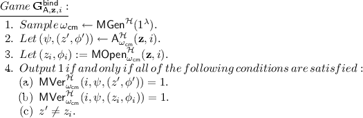
• Binding: For all $\mathbf {z} = (z_1,\ldots ,z_N)\in \{0,1\}^{kN}$, for all $i\in [N]$, and all PPT adversaries $\mathsf {A}$, we have $\Pr [\mathbf {G}^\mathsf{bind}_{\mathsf {A},\mathbf {z},i}(\lambda ) = 1] \le \nu _\mathsf{mt}$, where the game $\mathbf {G}^\mathsf{bind}_{\mathsf {A},\mathbf {z},i}(\lambda )$ is defined as follows:

  

The standard hash-tree construction due to Merkle [36] gives us a $(k,k,N,O(k\log (N)),\mathrm{negl}(k))$-Merkle Commitment.

4.3 Graph Pebbling and Labeling

Throughout this paper $G=(V,E)$ is considered to be a directed acyclic graph (DAG), where V is the set of vertices and E is the set of edges of the graph G. Without loss of generality we assume that the vertices of G are ordered lexicographically and are represented by integers in $[N]$, where $N= \vert V \vert$. Vertices with no incoming edges are called input vertices or sources, and vertices with no outgoing edges are called output vertices or sinks. We denote ${\varGamma ^{-}}(v)$, the set of all predecessors of the vertex v. Formally, ${\varGamma ^{-}}(v) = \{ w \in V :(w,v) \in E\}$.

In this section we briefly explain the concept of graph labeling and its connection to the abstract game called graph pebbling which has been introduced in [17]. For more details we refer to previous literature in, e.g., [4, 17, 18, 40]. We follow conventions from [40] and will use results from the same. Sometimes for completeness we will use texts verbatim from the same paper.

Labeling of a graph. Let $\mathcal {H}:\{0,1\}^{*}\rightarrow \{0,1\}^{{n_{\mathcal {H}}}}$ be a random oracle. The $\mathcal {H}$-labeling of a graph G is a function which assigns a label to each vertex in the graph; more precisely, it is a function $\mathsf {label}:V \rightarrow \{0,1\}^{{n_{\mathcal {H}}}}$ which maps each vertex $v \in V$ to a bit string $\mathsf {label}(v) :=\mathcal {H}(q_{v})$, where we denote by $\left\{ v^{(1)}, \dots , v^{(d)}\right\} = {\varGamma ^{-}}(v)$ and let

$$\begin{aligned} q_{v} :={\left\{ \begin{array}{ll} v~~\text { if } v \text { is an input vertex},\\ v\ || \ \mathsf {label}(v^{(1)})\ ||\ \dots \ || \ \mathsf {label}(v^{(d)}) &{} \text {otherwise}. \end{array}\right. } \end{aligned}$$

An algorithm $\mathsf {A}^\mathcal {H}$ labels a subset of vertices $W \subseteq V$ if it computes $\mathsf {label}(W)$. Specifically, $\mathsf {A}^{\mathcal {H}}$ labels the graph G if it computes $\mathsf {label}(V)$.

Additionally, for $m \le \vert V \vert$, we define the $\mathcal {H}$-labeling of the graph G with m faults¹⁴ as a function $\mathsf {label}:V \rightarrow \{0,1\}^{{n_{\mathcal {H}}}}$ such that, for some subset of vertices $M \subset V$ of size m, it holds $\mathsf {label}(v)=\mathcal {H}(q_{v})$ for every $v \in V \setminus M$, and $\mathsf {label}(v)\ne \mathcal {H}(q_{v})$ for every $v \in M$. Sometimes we refer to labeling with faults as partial labeling. The following lemma appeared in form of a discussion in [40]. It is based on an observation previously made in [18].

Lemma 1

([40, Sect. 5.2]). Let $\mathsf {A}^\mathcal {H}$ be an $(s,t)$-bounded algorithm which computes the labeling of a DAG G with $m\in \mathbb {N}$ faults. Then there exists an $(s+ m\cdot {n_{\mathcal {H}}},t)$-bounded algorithm $\tilde{\mathsf {A}}^\mathcal {H}$ that computes the labeling of $G$ without faults but gets $m$ correct labels to start with (they are initially stored in the memory of $\tilde{\mathsf {A}}^\mathcal {H}$ and sometimes called initial labels).

Intuitively the above lemma follows because the algorithm $\tilde{\mathsf {A}}^\mathcal {H}$ can overwrite the additional space it has, once the initial labels stored there are not needed.

Pebbling game. The pebbling of a DAG $G=(V,E)$ is defined as a single-player game. The game is described by a sequence of pebbling configurations $\mathbf {P}=(P_{0}, \dots , P_{T})$, where $P_{i}\subseteq V$ is the set of pebbled vertices after the i-th move. In our model, the initial configuration $P_{0}$ does not need to be empty. The rules of the pebbling game are the following. During one move (translation from $P_{i}$ to $P_{i+1}$), the player can place one pebble on a vertex v if v is an input vertex or if all predecessors of v already have a pebble. After placing one pebble, the player can remove pebbles from arbitrary many vertices.¹⁵ We say that the sequence $\mathbf {P}$ pebbles a set of vertices $W \subseteq V$ if $W \subseteq \textstyle {\bigcup _{i \in [0,T]}} P_{i}$.

The time complexity of the pebbling game $\mathbf {P}$ is defined as the number of moves $t(\mathbf {P}):=T$. The space complexity of $\mathbf {P}$ is defined as the maximal number of pebbles needed at any pebbling step; formally, $s(\mathbf {P}):=\max _{i \in [0,T]} \{\vert P_{i} \vert \}$.

Ex-post-facto pebbling. Let $\mathsf {A}^{\mathcal {H}}$ be an algorithm that computes the (partial) $\mathcal {H}$-labeling of a DAG G. The ex-post-facto pebbling bases on the transcript of the graph labeling. It processes all oracle queries made by $\mathsf {A}^\mathcal {H}$ during the graph labeling (one at a time and in the order they were made). Informally, every oracle query of the form $q_{v}$, for some $v \in V$, results in placing a pebble on the vertex v in the ex-post-facto pebbling game. This provides us a link between labeling and pebbling of the graph G. The formal definition follows.

Let $\mathcal {H}:\{0,1\}^* \rightarrow \{0,1\}^{{n_{\mathcal {H}}}}$ be a random oracle and ${\mathcal {Q}_{\mathcal {H}}}$ a table of all random oracle calls made by $\mathsf {A}^{\mathcal {H}}$ during the graph labeling. Then we define the ex-post-facto pebbling $\mathbf {P}$ of the graph G as follows:

• The initial configuration $P_{0}$ contains every vertex $v\in V$ such that $\mathsf {label}(v)$ has been used for some oracle query (e.g. some query of the form $\mathcal {H}(\cdots \Vert \mathsf {label}(v)\Vert \cdots )$) at some point in the transcript but the query $q_{v}$ is not listed in the part of the transcript preceding such query.

• Assume that the current configuration is $P_{i}$, for some $i \ge 0$. Then find the next unprocessed oracle query which is of the form $q_{v}$, for some vertex v, and define $P_{i+1}$ as follows:

  • 1. Place a pebble on the vertex v.

  • 2. Remove all unnecessary pebbles. A pebble on a vertex v is called unnecessary if $\mathsf {label}(v)$ is not used for any future oracle query, or if the query $q_{v}$ is listed in the succeeding part of the transcript before $\mathsf {label}(v)$ is used in an argument of some other query later. Intuitively, either $\mathsf {label}(v)$ is never used again, or $\mathsf {A}^\mathcal {H}$ anyway queries $q_{v}$ before it is used again.

The lemma below appeared in several variations in the literature (see, for example, [4, 17, 40]), depending on the definition of graph pebbling.

Lemma 2

(Labeling Lemma). Let G be a DAG. Consider an $(s,t)$-bounded adversary $\mathsf {A}^\mathcal {H}$ which computes the $\mathcal {H}$-labeling of the graph G. Also assume that $\mathsf {A}^\mathcal {H}$ does not guess any correct output of $\mathcal {H}$ without querying it. Then the ex-post facto pebbling strategy $\mathbf {P}$ described above pebbles the graph G, and the complexity of $\mathbf {P}$ is $s(\mathbf {P})\le \frac{s}{{n_{\mathcal {H}}}}$ and $t(\mathbf {P})\le t$.

Proof

By definition of ex-post-facto pebbling, it is straightforward to observe that if $\mathsf {A}^\mathcal {H}$ computes the $\mathcal {H}$-labeling of the graph G, then the ex-post-facto pebbling $\mathbf {P}$ pebbles the graph. Since we assume that the adversary does not guess the correct label, the only way $\mathsf {A}^\mathcal {H}$ can learn the label of the vertex v is by querying the random oracle. The bound on $t(\mathbf {P})$ is immediate. Again, by definition of the ex-post-facto pebbling, there is no unnecessary pebble at any time. Thus, the number of required pebbles is equal to the maximum number of labels that $\mathsf {A}^\mathcal {H}$ needs to store at once. Hence, the space bound follows directly from the fact that each label consists of ${n_{\mathcal {H}}}$ bits and that the algorithm $\mathsf {A}^\mathcal {H}$ is $s$-space bounded.

Localized expander graphs. A $(\mu , \alpha , \beta )$-bipartite expander, for $0<\alpha<\beta <1$, is a DAG with $\mu$ sources and $\mu$ sinks such that any $\alpha \mu$ sinks are connected to at least $\beta \mu$ sources. We can define a DAG $G'_{\mu ,k_{G}, \alpha , \beta }$ by stacking $k_{G}$ ($\in \mathbb {N}$) bipartite expanders. Informally, stacking means that sinks of the i-th bipartite expander are sources of the i+1-st bipartite expander. It is easy to see that such a graph has $\mu (k_{G}+1)$ nodes which are partitioned into $k_{G}+1$ sets (which we call layers) of size $\mu$. A Stack of Localized Expander Graphs ($\text {SoLEG}$) is a DAG $G_{\mu ,k_{G},\alpha ,\beta }$ obtained by applying the transformation called localization (see [7, 40] for a definition) on each layer of the graph $G'_{\mu ,k_{G}, \alpha , \beta }$.

We restate two lemmas about pebbling complexity of $\text {SoLEG}$ from [40]. The latter appeared in [40] in form of a discussion.

Lemma 3

([40, Theorem 4]). Let $G_{\mu ,k_{G},\alpha ,\beta }$ be a $\text {SoLEG}$ where $\gamma :=\beta - 2 \alpha >0$. Let $\mathbf {P}=(P_{0}, \dots , P_{t(\mathbf {P})})$ be a pebbling strategy that pebbles at least $\alpha \mu$ output vertices of the graph $G_{\mu ,k_{G},\alpha ,\beta }$ which were not initially pebbled, where the initial pebbling configuration is such that $\vert P_{0} \vert \le \gamma \mu$, and the space complexity of $\mathbf {P}$ is bounded by $s(\mathbf {P})\le \gamma \mu$. Then the time complexity of $\mathbf {P}$ has the following lower bound: $t(\mathbf {P})\ge 2^{k_{G}} \alpha \mu$.

Lemma 4

([40, Sect. 5.2]. Let $G_{\mu ,k_{G},\alpha ,\beta }$ be a $\text {SoLEG}$ and $\mathcal {H}:\{0,1\}^{*}\rightarrow \{0,1\}^{{n_{\mathcal {H}}}}$ be a random oracle. There exists a polynomial time algorithm $\mathsf {A}^\mathcal {H}$ that computes the $\mathcal {H}$-labeling of the graph $G_{\mu ,k_{G},\alpha ,\beta }$ in $\mu {n_{\mathcal {H}}}$-space.

5 Non-Interactive Proofs of Space

5.1 NIPoS Definition

A proof of space (PoS) [4, 18] is a (possibly interactive) protocol between a prover and a verifier, in which the prover attempts to convince the verifier that it used a considerable amount of memory or disk space in a way that can be easily checked by the verifier. Here, “easily” means with a small amount of space and computation; a PoS with these characteristics is sometimes called a proof of transient space [40]. A non-interactive PoS (NIPoS) is simply a PoS where the proof consists of a single message, sent by the prover to the verifier; to each proof, it is possible to associate an identity.

Intuitively, a NIPoS should meet two properties known as completeness and soundness. Completeness says that a prover using a sufficient amount of space will always be accepted by the verifier. Soundness, on the other hand, ensures that if the prover invests too little space, it has a hard time to convince the verifier. A formal definition follows below.

Definition 9

(Non-interactive proof of space). For parameters $s_{\mathsf {P}},s_{\mathsf {V}},s,t,k,n\in \mathbb {N}$, with $s_{\mathsf {V}}\le s< s_{\mathsf {P}}$, and $\nu _\mathsf{pos}\in (0,1)$, an $(s_{\mathsf {P}},s_{\mathsf {V}},s,t,k,n,\nu _\mathsf{pos})$-non-interactive proof of space scheme (NIPoS for short) in the ROM consists of a tuple of PPT algorithms $(\mathsf {Setup}^\mathcal {H},\mathsf {P}^\mathcal {H},\mathsf {V}^\mathcal {H})$ with the following syntax.

• $\mathsf {Setup}^\mathcal {H}(1^\lambda )$: This is a randomized polynomial-time (in $\lambda$) algorithm with no space restriction. It takes as input the security parameter and it outputs public parameters $\omega _\mathsf{pos}\in \{0,1\}^*$.

• $\mathsf {P}^\mathcal {H}_{\omega _\mathsf{pos}}( id )$: This is a probabilistic polynomial-time (in $\lambda$) algorithm that is $s_{\mathsf {P}}$-bounded. It takes as input an identity $id \in \{0,1\}^k$ and hard-wired public parameters $\omega _\mathsf{pos}$, and it returns a proof of space $\pi \in \{0,1\}^n$.

• $\mathsf {V}^\mathcal {H}_{\omega _\mathsf{pos}}( id ,\pi )$: This algorithm is $s_{\mathsf {V}}$-bounded and deterministic. It takes as input an identity $id$, hard-wired public parameters $\omega _\mathsf{pos}$, and a candidate proof of space $\pi$, and it returns a decision bit.

We require the following properties to hold.

• Completeness: For all $id \in \{0,1\}^k$, we have that

  $$\Pr \left[ \mathsf {V}^\mathcal {H}_{\omega _\mathsf{pos}}( id ,\pi ) = 1:~\omega _\mathsf{pos}\leftarrow \mathsf {Setup}^\mathcal {H}(1^\lambda );\pi \leftarrow \mathsf {P}^\mathcal {H}_{\omega _\mathsf{pos}}( id )\right] = 1,$$

  where the probability is taken over the randomness of algorithms $\mathsf {Setup}$ and $\mathsf {P}$, and over the choice of the random oracle.

• Extractability: There exists a polynomial-time deterministic algorithm $\mathsf {K}$ (the knowledge extractor) such that for any probabilistic polynomial-time algorithm $\mathsf {B}$, and for any $id \in \{0,1\}^k$, we have

  $$\Pr [\mathbf {G}^\mathsf{ext}_{\mathsf {B}, id }(\lambda )= 1] \le \nu _\mathsf{pos},$$

  where the experiment $\mathbf {G}^\mathsf{ext}_{\mathsf {B}, id }(\lambda )$ is defined as follows:

  

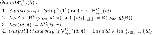
where $\mathsf {A}$ is an $(s,t)$-bounded deterministic algorithm, $q\in \mathrm {poly}(\lambda )$, the set ${\mathcal {Q}_{\mathcal {H}}}(\mathsf {B})$ contains the sequence of queries of $\mathsf {B}$ to $\mathcal {H}$ and the corresponding answers, and where the probability is taken over the coin tosses of $\mathsf {Setup},\mathsf {B},\mathsf {P}$, and over the choice of the random oracle.

Roughly, the extractability property requires that no space-bounded adversary is able to modify an honestly computed proof $\pi$ for identity $id$ into an accepting proof $\tilde{\pi }$ for an identity ${\tilde{ id }}\ne id$. Moreover, this holds true even if $\mathsf {A}$ is chosen adaptively (possibly depending on the public parameters, the identity $id$, and a corresponding valid proof $\pi$) by a PPT algorithm $\mathsf {B}$ with unbounded space. Since, however, $\mathsf {B}$ can compute offline an arbitrary polynomial number of valid proofs $( id _i,\pi _i)$, what the definition requires is that no $(\mathsf {B},\mathsf {A})$ is able to yield a valid pair $({\tilde{ id }},\tilde{\pi })$ for an ${\tilde{ id }}$ different than $id$ that the knowledge extractor $\mathsf {K}$ cannot predict by just looking at $\mathsf {B}$’s random oracle queries. It is easy to see that such an extractability requirement constitutes a stronger form of soundness, as defined, e.g., in [4, 40].

5.2 NIPoS Construction

We now give a NIPoS construction that is essentially a non-interactive variant of the PoS constructions of [40] that is in turn based on [4]. In particular, we show that it satisfies the stronger form of soundness which we call extractability. In addition, we formalize the security analysis given in [40] with concrete parameters that may be of independent interest.

The construction is built from the following ingredients:

• A random oracle $\mathcal {H}:\{0,1\}^*\rightarrow \{0,1\}^{n_{\mathcal {H}}}$.

• A graph $G_{\mu ,k_{G},\alpha ,\beta }$ from the family of $\text {SoLEG}$ (cf. Sect. 4.3), where $\alpha ,\beta$ are constants in (0, 1) such that $2\alpha < \beta$. By definition of such a graph, the number of nodes is given by $N= \mu (k_{G}+ 1)$. The in-degree $d$ depends on $\gamma = \beta - 2\alpha$, and it is hence constant.¹⁶

  Without loss of generality we assume that the vertices of $G_{\mu ,k_{G},\alpha ,\beta }$ are ordered lexicographically and are represented by integers in $[N]$. For simplicity we also assume that $N$ is a power of 2, and that $\log (N)$ divides ${n_{\mathcal {H}}}$.

• A $({n_{\mathcal {H}}},{n_\mathsf{cm}},N, {n_\mathsf{op}},\nu _\mathsf{mt})$-Merkle commitment scheme $(\mathsf {MGen}^\mathcal {H},\mathsf {MCommit}^\mathcal {H},\mathsf {MOpen}^\mathcal {H}, \mathsf {MVer}^\mathcal {H})$ (cf. Sect. 4.2).

Fig. 2.

Our NIPoS construction.

Our construction is formally described in Fig. 2. Let us here just briefly explain the main ideas. The setup algorithm chooses a graph $G_{\mu ,k_{G},\alpha ,\beta }$ from the family of $\text {SoLEG}$. Given an identity $id$, the prover first computes the $\mathcal {H}_{ id }$-labeling of the graph $G_{\mu ,k_{G},\alpha ,\beta }$ and commits to the resulting string using the Merkle commitment scheme. Then $\tau$ vertices of the graph are randomly chosen. For each challenged vertex v, the prover computes and outputs the opening for this vertex as well as opening for all its predecessors. The verifier gets as input the identity, a commitment, and $\tau (d+1)$ openings, where $d$ is the degree of the graph. It firstly verifies the consistency of all the openings with respect to the commitment. Secondly, it checks the local correctness of the $\mathcal {H}_{ id }$-labeling.

The completeness of our scheme relies on the correctness of the underlying commitment scheme. The extractability will follow from the pebbling complexity of the graph $G_{\mu ,k_{G},\alpha ,\beta }$ and the binding property of the commitment scheme. In particular, we prove the following statement:

Theorem 2

Let $\mathcal {H}:\{0,1\}^*\rightarrow \{0,1\}^{n_{\mathcal {H}}}$ be a random oracle, $G_{\mu ,k_{G},\alpha ,\beta }$ be a $\text {SoLEG}$ with $N= \mu (k_{G}+ 1)$ nodes and $d$ in-degree, and $(\mathsf {MGen}^\mathcal {H},\mathsf {MCommit}^\mathcal {H},\mathsf {MOpen}^\mathcal {H}, \mathsf {MVer}^\mathcal {H})$ be a $({n_{\mathcal {H}}},{n_\mathsf{cm}},N,{n_\mathsf{op}},\nu _\mathsf{mt})$-Merkle commitment. Let $s,t\in \mathbb {N}$ be such that, for some $\delta \in [0,\beta - 2\alpha )$, we have $t< 2^{k_{G}}\alpha \mu$ and $s\le \delta \mu {n_{\mathcal {H}}}$. Then, the NIPoS scheme described in Fig. 2 is a $(s_{\mathsf {P}},s_{\mathsf {V}},s,t,k,n,\nu _\mathsf{pos})$-NIPoS for any $k\in \mathbb {N}$, as long as:

$$\begin{aligned} s_{\mathsf {P}}&\ge k+ {n_{\mathcal {H}}}(\mu + \log (N) + 1) +n\\ s&\ge s_{\mathsf {V}}\ge k+ n+ {n_{\mathcal {H}}}\\ n&= {n_\mathsf{cm}}+ {n_\mathsf{op}}(d+1)({{n_{\mathcal {H}}}}/{\log (N)}) \\ \nu _\mathsf{pos}&\le \exp \left( \frac{-{n_{\mathcal {H}}}\mu (\gamma - \delta )}{N\log (N)}\right) + \frac{{n_{\mathcal {H}}}(d+1)\nu _\mathsf{mt}}{\log (N)} + \frac{\vert {\mathcal {Q}_{\mathcal {H}}}(\mathsf {A}) \vert }{2^{{n_{\mathcal {H}}}}}, \end{aligned}$$

where ${\mathcal {Q}_{\mathcal {H}}}(\mathsf {A})$ are the random oracle queries asked by $\mathsf {A}$ and $\gamma = \beta - 2\alpha$.

The formal proof appears in the full version. We provide some intuitions here. The adversary wins the game only if all the checked vertices have a correct $\mathcal {H}_{{\tilde{ id }}}$-label. By the binding property of the underlying Merkle commitment scheme this means that the adversary $\mathsf {A}$ has to compute a partial $\mathcal {H}_{{\tilde{ id }}}$-labeling of the graph $G_{\mu ,k_{G},\alpha ,\beta }$. Since ${\tilde{ id }}$ is not extractable from the query table of ${\mathcal {Q}_{\mathcal {H}}}(\mathsf {B})$ of the adversary $\mathsf {B}$ and it is not equal to $id$, the adversary $\mathsf {A}$ does not get any $\mathcal {H}_{{\tilde{ id }}}$ label “for free” and hence, it has to compute the labeling on its own. By Lemma 3, however, the labeling of the graph $G_{\mu ,k_{G},\alpha ,\beta }$ requires either a lot of space or a lot of time neither of which the $(s,t)$-bounded adversary $\mathsf {A}$ has. Instead of computing all the labels correctly via random oracle calls, the adversary $\mathsf {A}$ can assign labels of some vertices to an arbitrary value which does not need to be computed and stored. However, if such partial labeling consists of too many faults, the probability that at least one of the faulty vertices will be checked is high. Consequently, a winning adversary can not save a lot of recourses by computing only a partial labeling of the graph.

Using the parameters from Theorem 2 we obtain the following corollary.

Corollary 1

Let $\lambda \in \mathbb {N}$ be a security parameter. Let $\mathcal {H}:\{0,1\}^*\rightarrow \{0,1\}^{n_{\mathcal {H}}}$ be a random oracle, $G_{\mu ,k_{G},\alpha ,\beta }$ be a $\text {SoLEG}$ with $N= \mu (k_{G}+ 1)$ nodes and $d= O(1)$ in-degree, and $(\mathsf {MGen}^\mathcal {H},\mathsf {MCommit}^\mathcal {H},\mathsf {MOpen}^\mathcal {H}, \mathsf {MVer}^\mathcal {H})$ be a $({n_{\mathcal {H}}},{n_\mathsf{cm}},N,{n_\mathsf{op}},\nu _\mathsf{mt})$-Merkle commitment such that:

$$\begin{aligned} {n_{\mathcal {H}}}&= \lambda ^2&\gamma&= \beta - 2\alpha \in (0,1)&k_{G}&= \lambda -1&\mu&= \lambda ^3\\ {n_\mathsf{cm}}&= \lambda ^2&{n_\mathsf{op}}&= O(\lambda ^2\log (\lambda ))&\nu _\mathsf{mt}&\in \mathrm{negl}(\lambda ). \end{aligned}$$

Then, for any $\delta \in (0,\gamma )$, the scheme described in Fig. 2 is a $(s_{\mathsf {P}},s_{\mathsf {V}},s,t,k,n,\nu _\mathsf{pos})$-NIPoS, for $t\in \mathrm {poly}(\lambda )$ and

$$\begin{aligned} k&= O(\lambda ^4)&s_{\mathsf {P}}&= O(\lambda ^5)&s_{\mathsf {V}}&= O(\lambda ^4)\\ n&= O(\lambda ^4)&O(\lambda ^4) \le&s\le \delta \cdot \lambda ^5&\nu _\mathsf{pos}&\le \exp \left( \frac{-(\gamma -\delta )\lambda }{\log (\lambda )}\right) + \mathrm{negl}(\lambda ) \in \mathrm{negl}(\lambda ) \end{aligned}$$

6 Our Coding Scheme

6.1 Code Construction

Let $(\mathsf {Setup}^\mathcal {H}, \mathsf {P}^\mathcal {H},\mathsf {V}^\mathcal {H})$ be a NIPoS in the ROM where $\mathcal {H}:\{0,1\}^*\rightarrow \{0,1\}^{{n_{\mathcal {H}}}}$ denotes the random oracle for some ${n_{\mathcal {H}}}\in \mathrm {poly}(\lambda )$. We define a $(k,n)$-coding scheme $\varPi =(\mathsf {Init}^\mathcal {H}, \mathsf {Encode}^\mathcal {H}, \mathsf {Decode}^\mathcal {H})$ as follows.

• $\mathsf {Init}^\mathcal {H}(1^\lambda )$: Given as input a security parameter $\lambda$, it generates the public parameters for the NIPoS as $\omega _\mathsf{pos}\leftarrow \mathsf {Setup}^\mathcal {H}(1^\lambda )$, and outputs $\omega := \omega _\mathsf{pos}$.

• $\mathsf {Encode}^\mathcal {H}_{\omega }(x)$: Given as input the public parameters $\omega = \omega _\mathsf{pos}$ and a message $x\in \{0,1\}^{k}$, it runs the prover to generate the proof of space $\pi \leftarrow \mathsf {P}_{\omega _\mathsf{pos}}^\mathcal {H}(x)$ using the message $x$ as identity. Then it outputs $c:=(x,\pi ) \in \{0,1\}^{n}$ as a codeword.

• $\mathsf {Decode}^\mathcal {H}_{\omega }(c)$: Given a codeword $c$, it first parses $c$ as $(x,\pi )$. Then it runs the verifier $b:=\mathsf {V}_{\omega _\mathsf{pos}}^\mathcal {H}(x,\pi )$. If $b = 1$ it outputs $x$, otherwise it outputs $\bot$.

Theorem 3

Let $\lambda$ be a security parameter. Suppose that $(\mathsf {Setup}^\mathcal {H}, \mathsf {P}^\mathcal {H},\mathsf {V}^\mathcal {H})$ is a $(s_{\mathsf {P}},s_{\mathsf {V}},s,k_\mathsf{pos},n_\mathsf{pos},\mathrm{negl}(\lambda ))$-NIPoS. Then, for any $p\in \mathbb {N}$ such that $k_\mathsf{pos}+n_\mathsf{pos}\le p\le s$ and $\theta \in \mathrm {poly}(\lambda )$, the $(k,n)$-code $\varPi =(\mathsf {Init}^\mathcal {H}, \mathsf {Encode}^\mathcal {H},\mathsf {Decode}^\mathcal {H})$ defined above is an $(\ell ,s,p,\theta ,s_{\mathsf {V}})$-$\text {SP-NMC}$ in the ROM, where

$$k= k_\mathsf{pos}\qquad \qquad n= k_\mathsf{pos}+n_\mathsf{pos}\qquad \qquad \ell = \theta \cdot O(\log {\lambda }). $$

Recall that, in our definition of non-malleability, the parameter $s$ represents the space available for tampering, which is split into two components: $p$ bits of persistent space, which includes the $n$ bits necessary for storing the codeword and which is never erased, and $s-p$ bits of transient space that is erased after each tampering query.

Also, note that the above statement shows a clear tradeoff between the parameter $\theta$ (controlling the number of allowed tampering queries) and the leakage bound $\ell$. Indeed, the larger $\theta$, the more leakage we need, until the security guarantee becomes empty; this tradeoff is consistent with Theorem 1 (see also Fig. 1), as we know that leaky space-bounded non-malleability, for non-trivial values of $\ell$, is impossible for $p\approx n+ k$, whenever $\theta \ge k$.

6.2 Proof of Security

The correctness of the coding scheme is guaranteed by the perfect completeness of the NIPoS. Moreover, since the decoding algorithm simply runs the verifier of the $\text {NIPoS}$, it is straightforward to observe that decoding is $s_{\mathsf {V}}$ bounded.

Auxiliary algorithms. We start by introducing two auxiliary algorithms that will be useful in the proof. Recall that, by extractability of the $\text {NIPoS}$, there exists a deterministic polynomial-time algorithm $\mathsf {K}$ such that, given the public parameters $\omega _\mathsf{pos}$ and a table of RO queries ${\mathcal {Q}_{\mathcal {H}}}$, returns a set of identities $\{ id _i\}_{i \in [q]}$, for some $q\in \mathrm {poly}(\lambda )$. We define the following algorithms that use $\mathsf {K}$ as a subroutine.

• Algorithm $\mathsf {Find}(\omega _\mathsf{pos}, id ,{\mathcal {Q}_{\mathcal {H}}})$: Given a value $id \in \{0,1\}^{k_\mathsf{pos}}$, it first runs $\mathsf {K}$ to obtain $\{ id _i\}_{i \in [q]} := \mathsf {K}(\omega _\mathsf{pos},{\mathcal {Q}_{\mathcal {H}}})$. If there exists an index $i \in [q]$ such that $id = id _i$, then it returns the string $\mathsf {str}:=\mathsf {bit}(i) || 01$,¹⁷ where the function $\mathsf {bit}(\cdot )$ returns the binary representation of its input. Otherwise, the algorithm returns the flag $1^\ell$. Clearly, $\ell = \lceil \log (q)\rceil + 2$.

• Algorithm $\mathsf {Reconstruct}(\omega _\mathsf{pos},\mathsf {str},{\mathcal {Q}_{\mathcal {H}}})$: On receiving an $\ell$-bit string $\mathsf {str}$ and a RO query table ${\mathcal {Q}_{\mathcal {H}}}$, it works as follows depending on the value of $\mathsf {str}$:

  • - If $\mathsf {str}= 0^\ell$, output the symbol $\mathsf {same}^\star$.

  • - If $\mathsf {str}= 1^\ell$, output the symbol $\bot$.

  • - If $\mathsf {str}= a||01$, set $i :=\mathsf {bit}^{-1}(a)$. Hence, run algorithm $\mathsf {K}$ to get the set $\{ id _i\}_{i \in [q]} := \mathsf {K}(\omega _\mathsf{pos},{\mathcal {Q}_{\mathcal {H}}})$; in case $i \in [q]$, output the value $x := id _i$, otherwise output $\bot$.

  • Else, output $\bot$.

Constructing the simulator. We now describe the simulator $\mathsf {S}^\mathsf {D}= (\mathsf {S}_1^\mathsf {D},\mathsf {S}_2^\mathsf {D})$, depending on a PPT distinguisher $\mathsf {D}$.¹⁸ A formal description of the simulator is given in Fig. 3; we provide some intuitions below.

Informally, algorithm $\mathsf {S}_1$ simulates the random oracle $\mathcal {H}$ by sampling a random key ${\chi }\leftarrow \{0,1\}^{n_\mathsf{key}}$ for a pseudorandom function (PRF) $\mathsf {PRF}_{\chi }:\{0,1\}^*\rightarrow \{0,1\}^{n_{\mathcal {H}}}$; hence, it defines $\mathcal {H}(u) := \mathsf {PRF}_{\chi }(u)$ for any $u\in \{0,1\}^*$.¹⁹ $\mathsf {S}_2$ receives the description of the RO (i.e., the PRF key ${\chi }$) from $\mathsf {S}_1$, and for each tampering query $\mathsf {A}_i$ from $\mathsf {D}$ it asks a leakage query $L _i$ to its leakage oracle. The leakage query hard-codes the description of the simulated RO, the table ${\mathcal {Q}_{\mathcal {H}}}(\mathsf {D})$ consisting of all RO queries asked by $\mathsf {D}$ (until this point), and the code of all tampering algorithms $\mathsf {A}_1,\cdots ,\mathsf {A}_i$. Thus, $L _i$ first encodes the target message x to generate a codeword c, applies the composed function $\mathsf {A}_i\circ \mathsf {A}_{i-1}\circ \cdots \circ \mathsf {A}_1$ on c to generate the tampered codeword $\tilde{c}_i$, and decodes $\tilde{c}_i$ obtaining a value $\tilde{x}_i$. Finally, the leakage function signals whether $\tilde{x}_i$ is equal to the original message x, to $\bot$, or to some of the identities the extractor $\mathsf {K}$ would output given the list of $\mathsf {D}$’s RO queries (as defined in algorithm $\mathsf {Find}$). Upon receiving the output from the leakage oracle, $\mathsf {S}_2$ runs $\mathsf {Reconstruct}$ and outputs whatever this algorithm returns.

Fig. 3.

Description of the simulator $\mathsf {S}=(\mathsf {S}_1,\mathsf {S}_2)$

Some intuitions. Firstly, note that in the real experiment the random oracle is a truly random function, whereas in the simulation random oracle queries are answered using a PRF. However, using the security of the PRF, we can move to a mental experiment that is exactly the same as the simulated game, but replaces the PRF with a truly random function.

Secondly, a closer look at the algorithms $\mathsf {Find}$ and $\mathsf {Reconstruct}$ reveals that the only case in which the simulation strategy goes wrong is when the tampered codeword $\tilde{c}_i$ is valid, but the leakage corresponding to the output of $\mathsf {Find}$ provokes a $\bot$ by $\mathsf {Reconstruct}$ for some $i \in [\theta ]$. We denote this event as $\textsc {Fail}$. We prove that $\textsc {Fail}$ occurs exactly when the adversary $\mathsf {D}$ violates the extractibility property of the underlying $\text {NIPoS}$, which happens only with negligible probability.

To simplify the notation in the proof, let us write

$$ \mathsf {D}^\mathrm{cnm} :=\mathsf {D}^{\mathcal {H}(\cdot ),\mathcal {O}_\mathrm{cnm}^{\varPi ,x,\omega ,s,p}(\cdot )}, \ \mathsf {D}^{{\mathrm {sim}'}}:=\mathsf {D}^{\mathcal {H}(\cdot ),\mathcal {O}_\mathrm{sim}^{\mathsf {S}_2,\ell ,x,s,\omega }(\cdot )},\ \mathsf {D}^\mathrm{sim}:=\mathsf {D}^{\mathsf {S}_1(\cdot ),\mathcal {O}_\mathrm{sim}^{\mathsf {S}_2,\ell ,x,s,\omega }(\cdot )} $$

to denote the interaction in the real, resp. mental, resp. simulated experiment.

Formal analysis. Consider an adversary $\mathsf {D}$ which makes $\theta$ queries to $\mathcal {O}_\mathrm{cnm}$. By Definition 7, we need to prove that the simulator $\mathsf {S}^\mathsf {D}=(\mathsf {S}^\mathsf {D}_1, \mathsf {S}^\mathsf {D}_2)$ defined in Fig. 3 is such that, for all values $x\in \{0,1\}^{k}$, there is a negligible function $\nu :\mathbb {N}\rightarrow [0,1]$ satisfying

$$\begin{aligned} \big |\mathrm {Pr}\left[ \mathsf {D}^\mathrm{cnm}(\omega ) = 1:\omega \leftarrow \mathsf {Init}^\mathcal {H}(1^\lambda )\right] - \mathrm {Pr}\left[ \mathsf {D}^\mathrm{sim}(\omega ) = 1:\omega \leftarrow \mathsf {Init}^{\mathsf {S}_1}(1^\lambda )\right] \big | \le \nu (\lambda ). \end{aligned}$$

A straightforward reduction to the pseudorandomness of the PRF yields:

$$\begin{aligned} \left| \mathrm {Pr}\left[ \mathsf {D}^\mathrm {sim}(\omega ) = 1:\omega \leftarrow \mathsf {Init}^{\mathsf {S}_1}(1^\lambda )] - \Pr [\mathsf {D}^{\mathrm {sim}'}(\omega )=1:\omega \leftarrow \mathsf {Init}^\mathcal {H}(1^\lambda )\right] \right| \le \nu '(\lambda ), \end{aligned}$$

where $\nu ':\mathbb {N}\rightarrow [0,1]$ is a negligible function.

Let us now fix some arbitrary $x\in \{0,1\}^{k}$. For every $i \in [\theta ]$, we recursively define the event $\textsc {NotExtr}_i$ as:

$$\begin{aligned} \textsc {NotExtr}_i&:=\lnot \textsc {NotExtr}_{i-1} \ \wedge \ \mathsf {Decode}^{\mathcal {H}}_\omega (\tilde{c}) \not \in \{\bot ,x\} \\&\qquad \qquad \qquad \wedge \ \mathsf {Find}(\omega , \mathsf {Decode}^{\mathcal {H}}_\omega (\tilde{c}),{\mathcal {Q}_{\mathcal {H}}}(\mathsf {D})) = 1^\ell , \end{aligned}$$

where $\textsc {NotExtr}_0$ is an empty event that never happens and $(\tilde{c}, \tilde{\sigma }) :=\widetilde{\mathsf {A}}_i(c,\sigma )$ for $\widetilde{\mathsf {A}}_i :=\mathsf {A}_i\circ \mathsf {A}_{i-1}\circ \cdots \circ \mathsf {A}_1$. In other words, the event $\textsc {NotExtr}_i$ happens when $\mathsf {A}_i$ is the first adversary that tampers to a valid codeword of a message $\tilde{x}\ne x$ which is not extraxtable from ${\mathcal {Q}_{\mathcal {H}}}(\mathsf {D})$. In addition, we define the event

$$ \textsc {Fail}:=\bigvee _{i \in [\theta ]} \textsc {NotExtr}_i. $$

Now, we can bound the probability that $\mathsf {D}$ succeeds as follows:

$$\begin{aligned}&\left| \mathrm {Pr}\left[ \mathsf {D}^\mathrm{cnm}(\omega ) = 1\right] - \mathrm {Pr}\left[ \mathsf {D}^{{\mathrm {sim}'}}(\omega ) = 1\right] \right| \\&~\le ~\Big |\mathrm {Pr}\left[ \mathsf {D}^\mathrm{cnm}(\omega ) = 1 \mid \lnot \textsc {Fail}\right] -\mathrm {Pr}\left[ \mathsf {D}^{{\mathrm {sim}'}}(\omega ) = 1 \mid \lnot \textsc {Fail}\right] \Big | \cdot \Pr [\lnot \textsc {Fail}]\nonumber \\&\qquad + \Big |\mathrm {Pr}\left[ \mathsf {D}^\mathrm{cnm}(\omega ) = 1 \mid \textsc {Fail}\right] -\mathrm {Pr}\left[ \mathsf {D}^{{\mathrm {sim}'}}(\omega ) = 1 \mid \textsc {Fail}\right] \Big | \cdot \Pr [\textsc {Fail}]\nonumber \\&~\le ~\left| \mathrm {Pr}\left[ \mathsf {D}^\mathrm{cnm}(\omega ) = 1 \mid \lnot \textsc {Fail}\right] - \mathrm {Pr}\left[ \mathsf {D}^{{\mathrm {sim}'}}(\omega ) = 1 \mid \lnot \textsc {Fail}\right] \right| + \Pr [\textsc {Fail}],\nonumber \end{aligned}$$

(1)

where in the above equations the probability is taken also on the sampling of $\omega \leftarrow \mathsf {Init}^\mathcal {H}(1^\lambda )$. We complete the proof by showing the following two claims.

Claim

Event $\textsc {Fail}$ happens with negligible probability.

Proof

Assume that for some $x\in \{0,1\}^k$ adversary $\mathsf {D}$ provokes the event $\textsc {Fail}$ with non-negligible probability. This implies that there is at least one index $j\in [\theta ]$ such that event $\textsc {NotExtr}_j$ happens with non-negligible probability. We construct an efficient algorithm $\mathsf {B}$ running in game $\mathbf {G}^\mathsf{ext}_{\mathsf {B},x}(\lambda )$, that attempts to break the extractability of the NIPoS:

We observe that $\mathsf {B}$ perfectly simulates the view of $\mathsf {D}^{\mathrm {sim}'}$. So, if there exists at least one $j\in [\theta ]$ for which $\textsc {NotExtr}_j$ happens, $\mathsf {B}$ wins the game $\mathbf {G}^\mathsf{ext}_{\mathsf {B},x}(\lambda )$.

Therefore we have that $\Pr [\mathbf {G}^\mathsf{ext}_{\mathsf {D},x}(\lambda )= 1] \ge \Pr [\exists j\in [\theta ]:~\textsc {NotExtr}_j]$ which, combined with the extractability of $\text {NIPoS}$, completes the proof.

Claim

$\left| \mathrm {Pr}\left[ \mathsf {D}^\mathrm{cnm}(1^\lambda ) = 1 \mid \lnot \textsc {Fail}\right] - \mathrm {Pr}\left[ \mathsf {D}^{{\mathrm {sim}'}}(1^\lambda ) = 1 \mid \lnot \textsc {Fail}\right] \right| =0$

Proof

By inspection of the simulator’s description it follows that, conditioning on event $\textsc {Fail}$ not happening, the simulation oracle using $\mathsf {S}_2$ yields a view that is identical to the one obtained when interacting with the tampering oracle. The claim follows.

Combining the above two claims together with Eq. (1), we obtain that

$$ \left| \mathrm {Pr}\left[ \mathsf {D}^\mathrm{cnm}(\omega ) = 1:~\omega \leftarrow \mathsf {Init}^\mathcal {H}(1^\lambda )\right] - \mathrm {Pr}\left[ \mathsf {D}^{{\mathrm {sim}'}}(\omega ) = 1:~\omega \leftarrow \mathsf {Init}^{\mathsf {S}_1}(1^\lambda )\right] \right| $$

is negligible, as desired.

It remains to argue about the size of leakage. To this end, it suffices to note that the simulator $\mathsf {S}_2$ receives $O(\log (\lambda ))$ bits of leakage for every $i \in [\theta ]$. Thus, the total amount of leakage is $\theta \cdot O(\log (\lambda ))$, exactly as stated in the theorem.

6.3 Concrete Instantiation and Parameters

Instantiating Theorem 3 with our concrete $\text {NIPoS}$ from Corollary 1, and using bounds from Theorem 1, we obtain the following corollaries. The first corollary provides an upper bound on the number of tolerated tampering queries at the price of a high (but still non-trivial) leakage parameter.

Corollary 2

For any $\gamma ,\delta ,\varepsilon \in (0,1)$, there exists an explicit construction of a (k, n)-code in the ROM that is a $(\gamma \cdot k,s,p,\theta ,\varTheta (\lambda ^4))$-$\text {SP-NMC}$, where

$$k= \varTheta (\lambda ^4) \qquad n= \varTheta (\lambda ^4) \qquad \varTheta (\lambda ^4)\le p\le s= \delta \lambda ^5 \quad \theta = \varTheta (\lambda ^{4-\varepsilon }).$$

The second corollary yields a smaller number of tolerated tampering queries with optimal (logarithmic) leakage parameter.

Corollary 3

For any $\delta \in (0,1)$, there exists an explicit construction of a (k, n)-code in the ROM that is an $(O(\log \lambda ),s,p,\theta ,O(\lambda ^4))$-$\text {SP-NMC}$, where

$$k= O(\lambda ^4) \qquad n= O(\lambda ^4) \qquad O(\lambda ^4)\le p\le s= \delta \lambda ^5 \quad \theta = O(1).$$

7 Trading Leakage for Tamper-Proof Security

We revise the standard application of non-malleable codes to obtain protection against memory tampering attacks. The main idea, put forward in [21], is very simple. Let $\mathcal {F}$ be an arbitrary functionality, initialized with “secret key” $\kappa$; instead of storing $\kappa$, we store an encoding c of $\kappa$, computed via a non-malleable code. Hence, whenever we have to run $\mathcal {F}$, we decode c obtaining a value $\tilde{\kappa }$ which we use to evaluate the functionality on any chosen input. It is not too hard to show that this idea yields security against tampering attacks against the secret key, for the same class of adversaries supported by the non-malleable code.

This methodology, also known as “tamper simulatability”, has been explored in several variants [13, 25, 26, 35]. Here, we propose yet another variant where the above compiler is instantiated using a leaky space-bounded continuously non-malleable code; this yields security in a model where it is possible to “trade” security against space-bounded memory tampering, with some bits of leakage on the secret key, an idea already explored in a related line of research [28].

7.1 Leaky Tamper Simulatability

Let $\mathcal {F}:\{0,1\}^k\times \{0,1\}^{k_\mathsf{in}}\rightarrow \{0,1\}^{k_\mathsf{out}}$ be a randomized functionality, taking as input a secret value $\kappa \in \{0,1\}^k$ and a string $m\in \{0,1\}^{k_\mathsf{in}}$, and producing a value $y \leftarrow \mathcal {F}(\kappa ,m)\in \{0,1\}^{k_\mathsf{out}}$. For simplicity, we consider the case of stateless functionalities where the value $\kappa$ is never updated during the computation; an extension to the case of stateful functionalities is immediate, along the lines of previous work [21, 25, 35]. We note, however, that since updating the value $\kappa$ requires execution of the encoding algorithm (which uses a lot of space), considering only stateless functionalities is natural in our model.

Given a non-malleable code $\varPi$, the hardened functionality corresponding to $\mathcal {F}$ is defined below. For consistency with the rest of the paper, we state the definition in the ROM.

Definition 10

(Hardened functionality). Consider a functionality $\mathcal {F}:\! \{0,1\}^k\times \{0,1\}^{k_\mathsf{in}}\rightarrow \{0,1\}^{k_\mathsf{out}}$, and let $\varPi = (\mathsf {Init}^\mathcal {H},\mathsf {Encode}^\mathcal {H},\mathsf {Decode}^\mathcal {H})$ be a $(k,n)$-code in the ROM. For parameters $s,p\in \mathbb {N}$, with $s\ge p\ge n$, the $(s,p)$-memory hardened functionality $\hat{\mathcal {F}}(\varPi ,s,p)$ corresponding to $\mathcal {F}$ consists of algorithms $(\mathsf {Setup}^\mathcal {H},\mathsf {Run}^\mathcal {H})$ with the following syntax.

• $\mathsf {Setup}^\mathcal {H}(1^\lambda ,s,\kappa )$: Upon input the security parameter $\lambda \in \mathbb {N}$, sample $\omega \leftarrow \mathsf {Init}^\mathcal {H}(1^\lambda )$, let $c\leftarrow \mathsf {Encode}^\mathcal {H}_{\omega }(\kappa )$, and set $\mathcal {M}:= c||0^{p-n}||0^{s-p}$. Output $(\omega ,\mathcal {M})$.

• $\mathsf {Run}^\mathcal {H}_{\omega }(\mathcal {M},m)$: Parse $\mathcal {M}:= c||\sigma _0||\sigma _1$ and let $\tilde{\kappa } = \mathsf {Decode}^\mathcal {H}_{\omega }(c)$. If $\tilde{\kappa } = \bot$, set $\tilde{y}=\bot$; else, run $\tilde{y} \leftarrow \mathcal {F}(\tilde{\kappa },m)$. Update $\mathcal {M}:= c||\sigma _0||0^{s-p}$ and output $(\tilde{y},\mathcal {M})$.

It follows by correctness of the encoding scheme that, for all inputs, $\hat{\mathcal {F}}(\varPi ,s,p)$ computes exactly the same functionality as $\mathcal {F}$. Notice that the hardened functionality corresponding to $\mathcal {F}$ has $p$ bits of persistent storage (i.e., $n$ bits for storing the secret encoding and $p-n$ bits for auxiliary data); the remaining $s-p$ bits represent transient storage that is needed for decoding the codeword and running the original functionality with the obtained key (this memory is erased after each evaluation).

In case there is not enough transient space to decode or to run the original functionality, an external memory must be used. Thus, we get a natural trade-off between the amount of auxiliary data that can be stored on the device and the class of functionalities that can be executed without using an external memory.

Tampering experiment. To define security, we consider an $s$-bounded adversary that tampers with the memory content of the hardened functionality. This is done via the experiment described below, which is executed by a PPT algorithm $\mathsf {D}$, and is parametrized by an $(s,p)$-memory hardened functionality $\hat{\mathcal {F}}(\varPi ,s,p)$, a key $\kappa \in \{0,1\}^k$, a parameter $\theta \in \mathbb {N}$, and security parameter $\lambda \in \mathbb {N}$.

Leaky simulation. Intuitively, a non-malleable code is $\ell$-leaky tamper simulatable if the above tampering experiment can be simulated with black-box access to the original functionality $\mathcal {F}$, plus $\ell$ bits of leakage on the secret key. This is formalized in the experiment described below, which is executed by a PPT algorithm $\mathsf {D}$ and is parametrized by a functionality $\mathcal {F}$, a PPT simulator $\mathsf {S}$, a value $\ell \in \mathbb {N}$, an initial key $\kappa \in \{0,1\}^k$, a parameter $\theta \in \mathbb {N}$, and security parameter $\lambda \in \mathbb {N}$.

$\underline{\mathrm{Experiment}\,\, \mathbf {BBLeak}(\mathsf {D},\mathcal {F},\mathsf {S},\ell ,\kappa ,\theta ,\lambda ):}$

• 1. The simulator $\mathsf {S}$, which is given black-box access to $\mathcal {F}(\kappa ,\cdot )$ and oracle access to $\mathcal {O}_\mathrm{leak}^{\ell ,\kappa }(\cdot )$, emulates the entire view of $\mathsf {D}$. In particular:

  • It takes care of simulating the public parameters and answering (polynomially many) random oracle queries;

  • It needs to answer (at most $\theta$) tampering queries and (polynomially many) execute queries.

• 2. $\mathsf {D}$ outputs a bit as a function of its view.²⁰

Definition 11

(Leaky tamper simulatability). Let $\ell ,s,p,\theta ,k,n\in \mathbb {N}$ be functions of the security parameter $\lambda \in \mathbb {N}$, with $s\ge p\ge n$. A $(k,n)$-code $\varPi$ is $\ell$-leaky $(s,p)$-space $\theta$-tamper simulatable in the ROM, if for all PPT distinguishers $\mathsf {D}$ there exists a PPT simulator $\mathsf {S}$ such that for all functionalities $\mathcal {F}$, and for all $\kappa \in \{0,1\}^k$, there is a negligible function $\nu :\mathbb {N}\rightarrow [0,1]$ for which

$$\begin{aligned}&\Big |\mathrm {Pr}\left[ \mathbf {TamperInteract}(\mathsf {D},\hat{\mathcal {F}}(\varPi ,s,p),\kappa ,\theta ,\lambda )=1\right] \\&\qquad \qquad \qquad \qquad \qquad \qquad - \mathrm {Pr}\left[ \mathbf {BBLeak}(\mathsf {D},\mathcal {F},\mathsf {S},\ell ,\kappa ,\theta ,\lambda )=1\right] \Big \vert \le \nu (\lambda ). \end{aligned}$$

7.2 Analysis

In the following theorem, the proof of which appears in the full version, we show the correspondence between leaky non-malleable and leaky tamper simulatable codes.

Theorem 4

Let $\varPi$ be an $\ell$-leaky $(s,p)$-space-bounded $\theta$-continuously non-malleable code in the ROM. Then, $\varPi$ is also $\ell$-leaky $(s,p)$-space $\theta$-tamper simulatable in the ROM.

Informally, Theorem 4 states that every functionality $\mathcal {F}$ that is resistant to $\ell$ bits of leakage on the secret key can be protected against memory tampering by an $\ell$-leaky non-malleable code.

References

Aggarwal, D., Dodis, Y., Kazana, T., Obremski, M.: Non-malleable reductions and applications. In: STOC, pp. 459–468 (2015)
Aggarwal, D., Dodis, Y., Lovett, S.: Non-malleable codes from additive combinatorics. In: STOC, pp. 774–783 (2014)
Anderson, R., Kuhn, M.: Tamper resistance: a cautionary note. In: WOEC. USENIX Association, Berkeley (1996)
Ateniese, G., Bonacina, I., Faonio, A., Galesi, N.: Proofs of space: when space is of the essence. In: Abdalla, M., Prisco, R. (eds.) SCN 2014. LNCS, vol. 8642, pp. 538–557. Springer, Cham (2014). doi:10.1007/978-3-319-10879-7_31
Ball, M., Dachman-Soled, D., Kulkarni, M., Malkin, T.: Non-malleable codes for bounded depth, bounded fan-in circuits. In: Fischlin, M., Coron, J.-S. (eds.) EUROCRYPT 2016. LNCS, vol. 9666, pp. 881–908. Springer, Heidelberg (2016). doi:10.1007/978-3-662-49896-5_31
Bhattacharyya, R., Mukherjee, P.: Non-adaptive programmability of random oracle. Theor. Comput. Sci. 592, 97–114 (2015)
Boneh, D., Corrigan-Gibbs, H., Schechter, S.: Balloon hashing: a memory-hard function providing provable protection against sequential attacks. In: Cheon, J.H., Takagi, T. (eds.) ASIACRYPT 2016. LNCS, vol. 10031, pp. 220–248. Springer, Heidelberg (2016). doi:10.1007/978-3-662-53887-6_8
Boneh, D., DeMillo, R.A., Lipton, R.J.: On the importance of eliminating errors in cryptographic computations. J. Cryptology 14(2), 101–119 (2001)
Chattopadhyay, E., Goyal, V., Li, X.: Non-malleable extractors and codes, with their many tampered extensions. In: ACM STOC, pp. 285–298 (2016)
Cheraghchi, M., Guruswami, V.: Capacity of non-malleable codes. In: Innovations in Theoretical Computer Science, pp. 155–168 (2014)
Coretti, S., Dodis, Y., Tackmann, B., Venturi, D.: Non-malleable encryption: simpler, shorter, stronger. In: Kushilevitz, E., Malkin, T. (eds.) TCC 2016. LNCS, vol. 9562, pp. 306–335. Springer, Heidelberg (2016). doi:10.1007/978-3-662-49096-9_13
Coretti, S., Maurer, U., Tackmann, B., Venturi, D.: From single-bit to multi-bit public-key encryption via non-malleable codes. In: Dodis, Y., Nielsen, J.B. (eds.) TCC 2015. LNCS, vol. 9014, pp. 532–560. Springer, Heidelberg (2015). doi:10.1007/978-3-662-46494-6_22
Dachman-Soled, D., Liu, F.-H., Shi, E., Zhou, H.-S.: Locally decodable and updatable non-malleable codes and their applications. In: Dodis, Y., Nielsen, J.B. (eds.) TCC 2015. LNCS, vol. 9014, pp. 427–450. Springer, Heidelberg (2015). doi:10.1007/978-3-662-46494-6_18
Damgård, I., Faust, S., Mukherjee, P., Venturi, D.: The chaining lemma and its application. In: Information Theoretic, Security, pp. 181–196 (2015)
Damgård, I., Faust, S., Mukherjee, P., Venturi, D.: Bounded tamper resilience: How to go beyond the algebraic barrier. J. Cryptology 30(1), 152–190 (2017)
Dodis, Y., Yu, Y.: Overcoming weak expectations. In: Sahai, A. (ed.) TCC 2013. LNCS, vol. 7785, pp. 1–22. Springer, Heidelberg (2013). doi:10.1007/978-3-642-36594-2_1
Dwork, C., Naor, M., Wee, H.: Pebbling and proofs of work. In: Shoup, V. (ed.) CRYPTO 2005. LNCS, vol. 3621, pp. 37–54. Springer, Heidelberg (2005). doi:10.1007/11535218_3
Dziembowski, S., Faust, S., Kolmogorov, V., Pietrzak, K.: Proofs of space. In: Gennaro, R., Robshaw, M. (eds.) CRYPTO 2015. LNCS, vol. 9216, pp. 585–605. Springer, Heidelberg (2015). doi:10.1007/978-3-662-48000-7_29
Dziembowski, S., Kazana, T., Wichs, D.: Key-evolution schemes resilient to space-bounded leakage. In: Rogaway, P. (ed.) CRYPTO 2011. LNCS, vol. 6841, pp. 335–353. Springer, Heidelberg (2011). doi:10.1007/978-3-642-22792-9_19
Dziembowski, S., Kazana, T., Wichs, D.: One-time computable self-erasing functions. In: Ishai, Y. (ed.) TCC 2011. LNCS, vol. 6597, pp. 125–143. Springer, Heidelberg (2011). doi:10.1007/978-3-642-19571-6_9
Dziembowski, S., Pietrzak, K., Wichs, D.: Non-malleable codes. In: Innovations in Computer, Science, pp. 434–452 (2010)
Faonio, A., Nielsen, J.B., Venturi, D.: Mind your coins: fully leakage-resilient signatures with graceful degradation. In: Halldórsson, M.M., Iwama, K., Kobayashi, N., Speckmann, B. (eds.) ICALP 2015. LNCS, vol. 9134, pp. 456–468. Springer, Heidelberg (2015). doi:10.1007/978-3-662-47672-7_37
Faonio, A., Nielsen, J.B., Buus, J., Venturi, D.: Fully leakage-resilient signatures revisited: graceful degradation, noisy leakage, and construction in the bounded-retrieval model. Theor. Comput. Sci. 660, 23–56 (2017)
Faonio, A., Venturi, D.: Efficient public-key cryptography with bounded leakage and tamper resilience. In: Cheon, J.H., Takagi, T. (eds.) ASIACRYPT 2016. LNCS, vol. 10031, pp. 877–907. Springer, Heidelberg (2016). doi:10.1007/978-3-662-53887-6_32
Faust, S., Mukherjee, P., Nielsen, J.B., Venturi, D.: Continuous non-malleable codes. In: Lindell, Y. (ed.) TCC 2014. LNCS, vol. 8349, pp. 465–488. Springer, Heidelberg (2014). doi:10.1007/978-3-642-54242-8_20
Faust, S., Mukherjee, P., Nielsen, J.B., Venturi, D.: A tamper and leakage resilient von neumann architecture. In: Katz, J. (ed.) PKC 2015. LNCS, vol. 9020, pp. 579–603. Springer, Heidelberg (2015). doi:10.1007/978-3-662-46447-2_26
Faust, S., Mukherjee, P., Venturi, D., Wichs, D.: Efficient non-malleable codes and key derivation for poly-size tampering circuits. IEEE Trans. Inf. Theory 62(12), 7179–7194 (2016)
Faust, S., Pietrzak, K., Venturi, D.: Tamper-proof circuits: how to trade leakage for tamper-resilience. In: Aceto, L., Henzinger, M., Sgall, J. (eds.) ICALP 2011. LNCS, vol. 6755, pp. 391–402. Springer, Heidelberg (2011). doi:10.1007/978-3-642-22006-7_33
Fiat, A., Shamir, A.: How to prove yourself: practical solutions to identification and signature problems. In: Odlyzko, A.M. (ed.) CRYPTO 1986. LNCS, vol. 263, pp. 186–194. Springer, Heidelberg (1987). doi:10.1007/3-540-47721-7_12
Fischlin, M., Lehmann, A., Ristenpart, T., Shrimpton, T., Stam, M., Tessaro, S.: Random oracles with(out) programmability. In: Abe, M. (ed.) ASIACRYPT 2010. LNCS, vol. 6477, pp. 303–320. Springer, Heidelberg (2010). doi:10.1007/978-3-642-17373-8_18
Gennaro, R., Lysyanskaya, A., Malkin, T., Micali, S., Rabin, T.: Algorithmic tamper-proof (atp) security: theoretical foundations for security against hardware tampering. In: Naor, M. (ed.) TCC 2004. LNCS, vol. 2951, pp. 258–277. Springer, Heidelberg (2004). doi:10.1007/978-3-540-24638-1_15
Hazay, C., López-Alt, A., Wee, H., Wichs, D.: Leakage-resilient cryptography from minimal assumptions. In: Johansson, T., Nguyen, P.Q. (eds.) EUROCRYPT 2013. LNCS, vol. 7881, pp. 160–176. Springer, Heidelberg (2013). doi:10.1007/978-3-642-38348-9_10
Jafargholi, Z., Wichs, D.: Tamper detection and continuous non-malleable codes. In: Dodis, Y., Nielsen, J.B. (eds.) TCC 2015. LNCS, vol. 9014, pp. 451–480. Springer, Heidelberg (2015). doi:10.1007/978-3-662-46494-6_19
Katz, J., Vaikuntanathan, V.: Signature schemes with bounded leakage resilience. In: Matsui, M. (ed.) ASIACRYPT 2009. LNCS, vol. 5912, pp. 703–720. Springer, Heidelberg (2009). doi:10.1007/978-3-642-10366-7_41
Liu, F.-H., Lysyanskaya, A.: Tamper and leakage resilience in the split-state model. In: Safavi-Naini, R., Canetti, R. (eds.) CRYPTO 2012. LNCS, vol. 7417, pp. 517–532. Springer, Heidelberg (2012). doi:10.1007/978-3-642-32009-5_30
Merkle, R.C.: Method of providing digital signatures. US Patent 4309569, 5 January 1982
Mukherjee, P.: Protecting cryptographic memory against tampering attack. Ph.D thesis, Aarhus University (2015)
Naor, M., Segev, G.: Public-key cryptosystems resilient to key leakage. SIAM J. Comput. 41(4), 772–814 (2012)
Nielsen, J.B., Venturi, D., Zottarel, A.: Leakage-resilient signatures with graceful degradation. In: Krawczyk, H. (ed.) PKC 2014. LNCS, vol. 8383, pp. 362–379. Springer, Heidelberg (2014). doi:10.1007/978-3-642-54631-0_21
Ren, L., Devadas, S.: Proof of space from stacked expanders. In: Hirt, M., Smith, A. (eds.) TCC 2016. LNCS, vol. 9985, pp. 262–285. Springer, Heidelberg (2016). doi:10.1007/978-3-662-53641-4_11
Author information
Authors and Affiliations
Corresponding author
Editor information
Editors and Affiliations
Rights and permissions
Copyright information
© 2017 International Association for Cryptologic Research
About this paper
Cite this paper
Faust, S., Hostáková, K., Mukherjee, P., Venturi, D. (2017). Non-Malleable Codes for Space-Bounded Tampering. In: Katz, J., Shacham, H. (eds) Advances in Cryptology – CRYPTO 2017. CRYPTO 2017. Lecture Notes in Computer Science(), vol 10402. Springer, Cham. https://doi.org/10.1007/978-3-319-63715-0_4
Download citation
DOI: https://doi.org/10.1007/978-3-319-63715-0_4
Published:
Publisher Name: Springer, Cham
Print ISBN: 978-3-319-63714-3
Online ISBN: 978-3-319-63715-0
eBook Packages: Computer ScienceComputer Science (R0)