Retinal Vessel Classification Technique

Abstract

A retinal vessel classification procedure is proposed. From the image of thinned vessel network, landmarks are extracted and classified as branching, crossover and end points. Then a vascular graph is generated. Using a stratified graph edge labeling procedure the artery/vein map is built. In a first step the graph branches near the optic disc are localized and classified. Each label is propagated along the most significant segments linked to initial vessels. The next labeling phase aims the not processed branches starting from already classified vessels. Only branches and edges at crossings are labeled. Finally, using the current labels set, the uncertain cases are solved.

1 Introduction

The retinal vessel morphology can be modified by systemic diseases as diabetic retinopathy, glaucoma, atherosclerosis or macular degeneration. The arteries and veins are affected in different ways in such cases. For instance calibers of arteries decrease relatively to the calibers of veins. In other words the ratio between arteries and veins diameters (AVR) decreases. Another feature differently modified for arteries and veins is vessel tortuosity. To compute indicators as AVR or vessel tortuosity a classification of retinal vessels is mandatory. The vessel labeling phase is preceded by a complex task of retinal image processing and analysis: optic disc detection and modeling; vessel network segmentation; network landmarks (branching, crossover, end points) extraction and analysis; vessel graph generation and filtering. The main rules used by final labeling process are: a) the 3D vascular structure is cycle free, so each binary tree included in the 2D vessel graph represents a vessel; b) in the vicinity of the optic disc area vessels at crossings are of different type (an artery never crosses an artery, the same for veins).

Most of the proposed methods on the matter of artery/vein (A/V) classification localize in the vessel skeletons image branching, cross-over and end vessel points. Using these landmarks a graph reproducing the vessel network is synthesized. To eliminate the vessel network thinning errors and to simplify the graph different graph processing techniques have been proposed. In the final phase the A/V classification is performed by various graph analysis techniques. Subsequently some proposed methods following the above strategy are reviewed. In [1, 2] the graph is filtered to solve the errors eventually generated by vessel network thinning: splitting a real node in two (appears at the original large vessel intersections); missing links and false links. The graph analysis decides the type of each intersection point represented by the pertaining graph node. The 2nd degree nodes might be connecting or meeting points (where two vessels touch each other at their ends). Vessel crossings or tangential touches or splitting a vessel in two branches produce 3^rd degree nodes. Also, two vessels crossing each other or tangential touching each other (meeting point) or vessel splitting in three branches (bifurcation point) generate 4^th degree nodes. The 5^th degree nodes appear where more than two vessels are crossing. The nodes are classified as meeting or branch or cross point depending on the orientation and width of the incident vessel edges. According with the node type the incident edges are labeled as follows: (a) the same label as the current one at branching; (b) different label at crossings for two vessel segments and the same label for the fourth. In the last step, based on a combination of structural information and vessel intensity information, the domain of initial vessel labels is restricted to a binary domain (artery/vein). A comparison of results obtained using a supervised classification technique versus an unsupervised alternative is provided in [2]. Another artery/vein labeling approach is proposed in [3]. By Dijkstra’s shortest-path algorithm in the vascular graph vessel subtrees are identified and different sub-graphs are extracted. Each subgraph is labeled as artery or vein using a fuzzy C-mean clustering algorithm. In [4] the arteries and veins are classified employing a technique to extract the optimal forest in the graph given a set of constraints. A heuristically AC-3 algorithm to differentiate in the graph the two vessel classes is presented in [5]. Using some manually-labeled starting vessel segments the algorithm propagates the vessel labels as either artery or vein throughout the vascular tree. The A/V classification method proposed in [6] relies on estimating the overall vascular topology in order to finally label each individual vessel.

Some other proposed methods do not use the whole vessel graph to perform the A/V classification. For instance in [7], first the vessel network is extracted by a tracking technique. Then the optic disc is localized and its diameter approximated. A concentric zone around the optic disc is divided into four regions according to the position of the vessel network two main arcs. In every quadrant for each vessel a feature vector is synthesized. Finally, using a fuzzy clustering procedure each feature vector is allocated to one of the two classes. The same technique to separate the two vessel classes is employed by the author of [8] for AVR estimation. In [9] for each main vessel in a ring area around optic disc a six features vector has been constructed. The feature vector includes color intensities of the pixels representing the thinned vessel, the contrast differences in a 5 × 5 area of the vessel and in a 10 × 10 window outside the vessel. Finally a linear discriminant labels each feature vector as vein or artery. As in [7], the authors of [10] identify the optic disc and its approximate diameter. Then they divide the area around optic disc into four quadrants and for each quadrant vessel synthesize a feature vector. The feature vectors are labeled using a Gaussian Mixture Model and Expectation-Maximization unsupervised classifier.

Our first attempt to label the retinal vessels was presented in [11]. We proposed a stratified strategy based on main vessels identification located in the optic disc vicinity. Each main starting vessel is classified as vein or artery using a supervised classification technique. The established label is then propagated gradually along the most significant descendant vessels connected to the main branch. This way the eventually uncertain labeling cases appear in the last stages of the classification process for less significant vessels. To our knowledge this method leads to more accurate results than other proposed approaches on the A/V classification matter. In the next sections a new A/V classification approach with better performances versus the first version of the algorithm is presented. As in [11] to test the new method the manually segmented images of public DRIVE database were used as input. We resume from [11] all the image analysis steps: (a) the optic disc detection and modeling - the optic disc circle center and the circle radium r are used to crop on the segmented blood network image a circular ring bounded by two concentric circles centered in the optic disc center; the radii of the two circles are of 2r and 12r sizes [4, 12]; (b) in the selected area of segmented image: network landmark points detection and processing [13]; (c) new vessel’s graph analysis and classification.

The remainder of the paper is organized as follows. The preliminary image processing analysis to extract information used by the final classification is resumed from [11] in Sect. 2. The new vessel graph filtering approach is presented in Sect. 3. Section 4 details the new A/V classification procedure. The work is concluded in Sect. 5.

2 Preliminary Retinal Image Processing Steps

The working image synthesis is illustrated in Fig. 1:

Fig. 1.

Working area on four fundus images of drive database (area outside of inner circle and inside of outer circle) - upper row; manually segmented images - second row; thinning results - third row (TV); working images for landmarks detection (RV) - bottom row.

• 1. Using one of the techniques proposed in [12] the optic disc is detected and modeled. The radius r of the circle model is used as a parameter to extract the working area in the thinned image of the vessel network, Fig. 1 - upper and bottom rows;

• 2. From the DRIVE vessel images, figured by the second row of Fig. 1, a centerline image, denoted TV, is generated by thinning, Fig. 1 - third row;

• 3. A working image, noted RV, is built by deleting in TV image any vessel pixel outside the outer circle or inside the inner circle, Fig. 1 - bottom row.

Additionally two feature images are built, to be used in landmark analysis and final A/V classification:

• A vessel width image, denoted WV, is computed using the same technique described in [11];

• For each vessel pixel in TV image the intensity variance in the green channel of the original color image is computed, using a 14 × 14 window. The result is stored in a floating point array, noted VV.

3 Vessel Graph Processing

All nodes in the RV image are labeled as multiple and eventually essential, cross points (with more than three neighbors vessel points) according to the procedure presented in [4]. The multiple points set is ordered function of the point distance to optic disc center. Then the method proposed in [13] is employed to process multiple points in order to generate the significant crossover and bifurcation structure set. This procedure consists of the following main steps: (a) for each essential point the multiple neighbors are replaced by the nearest 2-neighbor vessel points on the branch; (b) if two nearby essential points share a starting point the two essential pixels become equivalent and only one would be validated, inheriting the starting points of the canceled essential pixel. It may happen that the valid essential point changes its status from branching to crossing pixel; (c) the essential points sharing all neighbors (starting points) with other essential pixels are canceled; (d) the branching points with a very short branch are canceled. For each significant point structure there are filled multiple point coordinates and the coordinates of the nearest 2-neighbor vessel pixels considered as starting points for vessel tracking in the RV image. For each starting point a tracking procedure is initiated. The tracking ends when another starting point or an end point (1 vessel neighbor) is met. Every tracking process generates a line structure which includes: line end points; essential points associated to end points; line length; tracked vessel pixel coordinates set; a binary attribute to mark the line as allocated (processed) during the graph structures generation process, presented in the next paragraph. Also, the line structure includes a graph index, to indicate the graph membership. Along the tracking for each vessel pixel the following parameters are grabbed from images generated in the process described in Sect. 2: vessel width (WV image); intensity variance (VV image); gray level of the correspondent pixel in green channel of the original RGB image. Subsequently for each line end the average of the above parameters are computed: (a) if the vessel length is greater than a threshold experimentally established, at each end a fraction of the stored vessel points are used to compute the parameter average; (b) for short segments the same procedure is employed using for both ends the whole set of vessel pixels. Then at each vessel end a slope is computed in the same manner as for width, intensity and variance intensity averages but this time using the coordinates of a fraction or of the whole set of stored vessel points. After the whole line structure set initialization each line structure is completed with pointers to the incident lines at its ends. For each incident line at crossings the associated line index structure field is completed if the two lines have almost the same width and local orientation.

Then the line structures are filtered according with the following rules:

• 1. At crossings of four or more lines delete weak lines (not aligned and very thin). For every deleted line update also the essential end points structure in order to rebuild the line structures;

• 2. At four lines crossings with two non-associated lines detect the weakest line from the two non-aligned lines. If one of the two aligned lines is short and the other end is a branch essential point it is possible to split the crossing in two branches. The closest new branch to the old branch of the short line might hide a crossing, (Fig. 2);

  Fig. 2.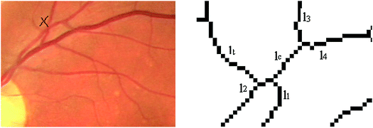

  

  Illustration of step 2 of the line structure filtering scheme. The vessel intersection is marked on the original image area – left figure. The crossing lines are figured on the right in the corresponding zoomed area of working image RV.

• 3. Find out eventually hidden crossings generated by short lines bounded by 3-connectivity essential points, (Fig. 3);

  Fig. 3.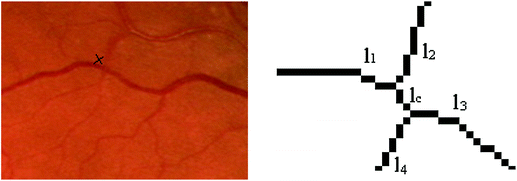

  

  Case 3 illustration of the line structure filtering scheme. The vessel intersection is marked on the original image area – left figure. The crossing lines are figured on the right in the intersection zoomed area of the working image RV.

• 4. Solve tangency for two cases:

  • 4.1. The tangency part is a short line with branching ends, [11];

  • 4.2. The tangency part is a short line with a branch at one end and four or more lines at the other end. At the end with more than four lines the largest two are selected and the problem is reduced to the precedent one, (Fig. 4).

    Fig. 4.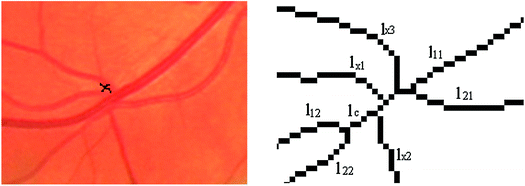

    

    Case 4.2 illustration of the line structure filtering scheme. The vessel intersection is marked on the original image area – left figure. The crossing lines are figured on the right in the intersection zoomed area of the working image RV.

• 5. Using a weaker condition find out the hidden crossings given by short lines bounded by 3-connectivity essential points, (Fig. 5).

  Fig. 5.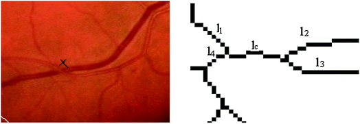

  

  Case 5 illustration of the line structure filtering scheme. The vessel intersection is marked on the original image area – left figure. The crossing lines are figured on the right in the intersection zoomed area of the working image RV.

The filtering procedure leads to completion of the association indices at line crossings, the same indices mentioned for direct line association at line structure synthesis - steps 1, 2, 3. In the same manner other two association line indices are filled: for tangency cases (4.1 and 4.2), and an index for association at crossings but for a more relaxed condition on line slopes - step 5. Except steps 1, 3 and 4.1, presented in [11], all the other procedures are new filtering approaches. The steps 2, 3 (resumed from [11]), 4.2 and 5 are illustrated in Figs. 2, 3, 4 and 5. The case 2, depicted by Fig. 2, is generated by a fake crossing of lines l₁, l₂, l_t and l_c. As shown in the left image of the original crossing area line l_t is a very thin one and the real crossing, hidden by line l_c, is of vessel of lines l₁ and l₃ with the vessel of lines l₂ and l₄.

Consequently the initial line association at the fake crossing is cancelled. The new one is set properly in the structures of lines l₁ and l₃ respectively l₂ and l₄, given the fact that the association conditions are fulfilled.

As mentioned in [11] for each line incident at crossings the associated line index structure field is completed if the two lines have almost the same width and local orientation. For the case depicted by Fig. 3 vessel of lines l₁ and l₃ is crossed by vessel of lines l₂ and l₄. In [11] there were treated tangency cases for short lines bounded by 3^rd degree nodes with the width significantly greater than the width of the incident lines, case 4.1 from above filtering scheme. In this paper we consider also the case of short lines thicker than each incident line bounded by a 3^rd degree node and a node with a degree greater than 3. This situation is illustrated in the right image of Fig. 4 where the line l _c is incident with lines l₁₂ and l₂₂ at one end and with l_x1, l_x2, l_x3, l₁₁ and l₂₁ lines at the other end. As mentioned above from the end with more than four lines the largest two are selected and the problem is reduced to the precedent one. In our case, from the node with l_x1, l_x2, l_x3, l₁₁ and l₂₁ lines the two widest lines are selected, respectively l₁₁ and l₂₁. If the association conditions for tangency of vessel l₁₁ and l₁₂ with vessel l₂₁ and l₂₂ there are fulfilled the rest of incident lines respectively l_x1, l_x2, l_x3 are placed in hold to be labeled in the last step of the classification process.

The last case of the line structures filtering is illustrated by Fig. 5. Using a weaker orientation line condition, there are identified the hidden crossings given by short lines bounded by 3-connectivity essential points. This time the lines l₁ and l₃, respectively l₂ and l₄ would finally be associated. At the second step of the labeling procedure the pairs of weak associated lines are placed in hold to be processed in the last phase of the process.

The final vessel segment graphs of the four working images set are illustrated on the bottom row of Fig. 6.

Fig. 6.

Vessel segment graphs (bottom row) of the four working image set (first row).

4 Stratified Vessel Classification Procedure

Starting from the line structures sets, illustrated by the bottom row of Fig. 6, graph structure sets are synthesized. Using the pointers to the incident lines at current line end by a tracking procedure the set of connected lines is marked with the same graph index. Also to avoid tracking cycles each line is marked as processed, once tracked. Then, for each line set with the same graph index there are identified the main branches starting from the inner circle of the working area. Each starting main branch is tracked in order to extract the rest of the vessel and to fill the graph structure. The following tracking rules are applied:

• 1. If at the current end of the current line only two child lines are linked choose the most significant vessel, with the largest width;

• 2. If at the current end are linked two branches having almost the same width choose the one with the closest slope to the mother line slope;

• 3. If at the current end are linked more than two branches choose as next branch the associated or weak associated line if there is an association at crossing;

• 4. If at crossings the current line is associated and the other pair is not, place the not-associated line in the holding list, to be labeled in the last step of the classification process;

• 5. If at crossings the current line has the tangency attribute set on, the next branch would be the associated segment;

• 6. If at crossings the current line has the complex tangency attribute set on, the next branch would be the associated segment and the other non-associated line indices would be placed in the holding list;

• 7. If all the lines at crossings are not associated choose the most significant vessel if there is one. Put the rest of lines in the holding list of unsolved pairs: each not chosen line makes pair with the current line;

• 8. If all the lines at crossings are not associated and the vessel width range is not large choose to associate to the current line the line with the most closed slope to the current one. Put the rest of incident lines in the list of unsolved pairs.

The graph structure and its completion are depicted below.

The graph structure generation pseudocode:

In order to initiate the vessel labeling process only the branches with a free end located in the optic disc vicinity are considered. For each starting main branch as many vessel segments are considered as their length sum is above a predefined threshold. For each main starting vessel of the graph a feature vector has been synthesized, with the following components: width, variance intensity, mean gray level. Previously more groups of statistical classifiers, differentiated by the vessel width range, have been trained using a feature vector set synthesized from images of public DRIVE database. The current feature vector is assigned by the designated supervised classifier to one of the two classes (“vein”, “artery”). In cases of uncertainty, when the vessel classification probability is low, the labeling is interactively accomplished. Once the starting vessel of a main branch has been labeled the established label is propagated along all segments of the branch. The result of main branch selection and labeling is illustrated by the bottom row of Fig. 7 (blue vessels are arteries, red vessels are veins).

Fig. 7.

The result of main branch selection (bottom row) for the four images set (first row).

The next labeling phase aims the branches starting from already classified main branches. This time the tracking rules are:

• 1. If at the current end of the current line are linked only two child lines choose the most significant vessel, with the largest width. The other child is placed in the stack to be labeled later;

• 2. If at the current end are linked two branches having almost the same width choose the one with the closest slope to the mother line slope. The other child is placed in the stack to be labeled later;

• 3. If at the current end are linked more than two branches choose as next branch the associated line if there is an association at crossing.

• 4. If at crossings the current line is associated and the other pair is not, place the not-associated line in the holding list, to be labeled in the last step of the classification process.

• 5. If at crossings the current line is weak associated place the pair in the holding list, to be labeled in the last step of the classification process. If the stack is not empty go on labeling the first line in the stack. Otherwise get the next graph labeled branch.

• 6. If at crossings the current line has the simple tangency attribute set on the next branch would be the associated segment.

• 7. If at crossings the current line has the complex tangency attribute set on place the pair in holding list together with the other non-associated lines indices. If the stack is not empty go on labeling the first line in the stack. Otherwise get the next graph labeled branch.

• 8. If all the lines at crossings are not associated place all children in the holding list of unsolved pairs: each child makes pair with the current line. If the stack is not empty go on labeling the first line in the stack. Otherwise get the next graph labeled branch.

The new labeling step pseudocode:

The result of labeling the vessels branching from main branches is depicted in Fig. 8.

Fig. 8.

The result of the second step of labeling process - bottom row; the result of main branch labeling is illustrated again on the upper row.

In the last labeling phase the list of unlabeled vessels completed during the first two steps would be processed. This time due to the fact that most part of vessel network is classified, so more information is available, the probability for a correct classification of the initially uncertain cases increases.

The following routine was implemented to complete the graph starting from a specific vessel and label. The completion might fail if during labelling already classified branches are met (Fig. 9).

Fig. 9.

The final result of the labeling process - bottom row; the result of previous labeling step is illustrated again on the upper row.

As we already mentioned to finalise the classification process all kind of uncertain cases are considered: non-associated lines at crossings collected in the first two steps and weak associated lines or complex tangency cases, grabbed in the second step. The algorithm pseudocode:

5 Conclusions

To assess the A/V classification the indicator $\text{R} = \frac{{\sum {\text{w}_{\text{i}} \text{l}_{\text{i}}^{{\text{cls}}} } }}{{\sum {\text{w}_{\text{j}} \text{l}_{\text{j}}^{{\text{init}}} } }}$ has been used, where $\text{l}_\text{i}^\text{cls}$ is the length of the correctly classified i^th vessel; $\text{l}_\text{j}^\text{init}$ is the length of j^th vessel from initial working image, depicted by the bottom row of Fig. 1. The vessel weight w _i is defined as: $\text{w}_{\text{i}} = 0.1 + 0.9\frac{{\text{width}_{\text{i}} - \text{width}_{\hbox{min} } }}{{\text{width}_{\hbox{max} } - \text{width}_{\hbox{min} } }}$., where width_i is the i^th vessel width, width_min is the minimum vessel width of the network and width_max is the maximum one.

Tests have been done on 20 manually segmented images from DRIVE database. The step of generating Line structures was flawless for the entire set. The classification rate was R = 0.95, better than the labeling rate R = 0.93 of the first version of the algorithm presented in [11].

Assuming a correct initial labeling of main vessels near the optic disc the stratified classification method leads to more accurate results than other proposed approaches on the A/V classification matter. As mentioned in [11] the eventually unsolved cases appear in the last stages of the labeling process for less significant vessels. However, the new algorithm performs a more reliable classification in certain cases and a more detailed selection of uncertain cases in its first two phases. After that more information is available so the probability for a correct classification of uncertain cases increases.

The reported work is a part of a larger project that will be completed later with the vessel network segmentation, to fulfill an artery/vein classification process.

The classification procedure was implemented in C++ and OpenCV library was used for image manipulation and some processing functions.

References

Dashtbozorg, B., Mendonça, A.M., Campilho, A.: An automatic graph-based approach for artery/vein classification in retinal images. IEEE Trans. Image Process. 23(3), 1073–1083 (2014)
Dashtbozorg, B.: Advanced image analysis for the assessment of retinal vascular changes. Ph.D. thesis, University of Porto (2015)
Joshi, V.S., Reinhardt, J.M., Garvin, M.K., Abramoff, M.D.: Automated method for identification and artery-venous classification of vessel trees in retinal vessel networks. PLoS ONE 9(2), e88061 (2014)
Lau, Q.P., Lee, M.L., Hsu, W., Wong, T.Y.: Simultaneously identifying all true vessels from segmented retinal images. IEEE Trans. Biomed. Eng. 60(7), 1851–1858 (2013)
Rothaus, K., Jiang, X., Rhiem, P.: Separation of the retinal vascular graph in arteries and veins based upon structural knowledge. Image Vis. Comput. 27, 864–875 (2009)
Estrada, R., Allingham, M.J., Mettu, P.S., Cousins, S.W., Tomasi, C., Farsiu, S.: Retinal artery-vein classification via topology Estimation. IEEE Trans. Med. Imaging 34(12), 2518–2534 (2015)
Grisan, E., Ruggeri, A.: A divide et impera strategy for automatic classification of retinal vessels into arteries and veins. In: Proceedings of the 25th Annual International Conference of the IEEE Engineering in Medicine and Biology Society, 2003, vol. 1, pp. 890–893 (2003)
De Luca, M.: New techniques for the processing and analysis of retinal images in diagnostic ophthalmology. Ph.D. thesis, University of Padova (2008)
Muramatsu, C., Hatanaka, Y., Iwase, T., Hara, T., Fujita, H.: Automated selection of major arteries and veins for measurement of arteriolar-to-venular diameter ratio on retinal fundus images. Comput. Med. Imag. Graph. 35(6), 472–480 (2011)
Relan, D., MacGillivray, T., Ballerini, L., Trucco, E.: retinal vessel classification: sorting arteries and veins. In: 2013 35th Annual International Conference of the IEEE Engineering in Medicine and Biology Society (EMBC), pp. 7396–7399 (2013)
Rotaru, F., Bejinariu, S.I., Luca, R., Niţă, C.: Retinal vessel labeling method. In: Proceedings 5th IEEE International Conference on E-Health Bioengineering, Iaşi, pp. 19–21 (2015)
Rotaru, F., Bejinariu, S.I., Nita, C.D., Luca, R., Luca, M., Ignat, A.: Optic disc recognition method for retinal images, soft computing applications volume 357 of the series Advances in Intelligent Systems and Computing, pp. 875–889. Springer, Heidelberg (2015)
Rotaru, F., Bejinariu, S., Bulea, M., Nita, C., Luca, R.: Vascular bifurcations and crossovers detection and processing in retinal images. In: Proceedings 12th International Symposium on Signals, Circuits and Systems (ISSCS 2015), Iasi (2015)
Acknowledgments
The work was done as part of research collaboration with University of Medicine and Pharmacy “Gr. T. Popa” Iaşi to analyse retinal images for early prevention of ophthalmic diseases.
Author information
Authors and Affiliations
Corresponding author
Editor information
Editors and Affiliations
Rights and permissions
Copyright information
© 2018 Springer International Publishing AG
About this paper
Cite this paper
Rotaru, F., Bejinariu, SI., Niţă, C.D., Luca, R., Luca, M., Ciobanu, A. (2018). Retinal Vessel Classification Technique. In: Balas, V., Jain, L., Balas, M. (eds) Soft Computing Applications. SOFA 2016. Advances in Intelligent Systems and Computing, vol 634. Springer, Cham. https://doi.org/10.1007/978-3-319-62524-9_37
Download citation
DOI: https://doi.org/10.1007/978-3-319-62524-9_37
Published:
Publisher Name: Springer, Cham
Print ISBN: 978-3-319-62523-2
Online ISBN: 978-3-319-62524-9
eBook Packages: EngineeringEngineering (R0)