Seismic Performance of RC Building Using Spectrum Response and Pushover Analyses

Abstract

Classical seismic design codes consider behavior factor to assess seismic response of structures proposing simplified equivalent static method and dynamic spectral modal method using response spectrum. Both use a global behavior factor to take into account nonlinear effect of elements response. Nowadays Performance based Seismic Design considers nonlinear static analyses using Pushover analysis with different performance levels. They permit to determine the bearing capacity of structures and distinguish whether they will be able to withstand major earthquakes. The first mode is in general considered in such kind of analysis.

This study will compare the shear base forces, drift and absolute displacements using dynamic response spectrum analysis and pushover analysis according to Eurocode 8. The results are carried in accordance with the Algerian seismic design Code in force RPA99/version 2003 and ETABS 2013 program.

These keywords were added by machine and not by the authors. This process is experimental and the keywords may be updated as the learning algorithm improves.

1 Introduction

The Algerian seismic code propose simplified methods to assess the response of structures under earthquakes actions, such as equivalent static method and spectrum response method which permit to evaluate first lateral forces, and then to check lateral displacements. The nonlinear behavior of dissipative elements is taken into account through the behavior factor R, which consider dissipative take. The 2003 Boumerdes major earthquake, magnitude 6.9 showed some shortcomings of these simplified methods. In the recent years, new methods of seismic assessment and design have been developed, particularly with respect to real nonlinear behavior of structural elements using nonlinear static analysis (pushover) with several performance levels. The basic theory consider capacity design approach. The literature propose many procedures like ATC40, FEMA 354, FEMA 440, N2 method (Eurocode 8).

1.1 Linear Response Spectrum Method

Response spectrum method is one of the useful tools of earthquake engineering for analyzing the performance of structures especially in earthquakes, since many systems behave as single degree of freedom systems. Thus, once the natural frequency of the structure evaluated, then the peak response of the building can be estimated by reading the value from the ground response spectrum for the appropriate frequency. In most building codes in seismic regions, this value forms the basis for calculating the forces that a structure must be designed to resist seismic analysis. Response spectrum method is a linear dynamic statistical analysis method which measures the contribution from each natural mode of vibration to indicate the likely maximum seismic response of an essentially elastic structure. Response spectrum analysis provides insight into dynamic behavior by measuring pseudo-spectral acceleration, velocity, or displacement as a function of structural period for a given time history and level of damping. It is practical to envelope response spectra such that a smooth curve represents the peak response for each realization of structural period (RPA 2003).

The seismic force is represented by using the following response spectrum from a ground motion:

$$ \frac{{{\text{S}}_{\text{a}} }}{\text{g}}\left\{ {\begin{array}{*{20}l} {1.25{\text{A}}\left( {1 + \frac{\text{T}}{{{\text{T}}_{1} }}\left( {2.5\upeta\frac{\text{Q}}{\text{R}} - 1} \right)} \right)} \hfill & {0 \le {\text{T}} \le {\text{T}}1} \hfill \\ {2.5\upeta\left( {1.25{\text{A}}} \right)\frac{\text{Q}}{\text{R}}} \hfill & {{\text{T}}_{1} \le {\text{T}} \le {\text{T}}_{2} } \hfill \\ {2.5\upeta\left( {1.25{\text{A}}} \right)\frac{\text{Q}}{\text{R}}(\frac{{{\text{T}}_{2} }}{\text{T}})^{{\frac{2}{3}}} } \hfill & {{\text{T}}_{2} \le {\text{T}} \le 3{\text{s}}} \hfill \\ {2.5\upeta\left( {1.25{\text{A}}} \right)\frac{\text{Q}}{\text{R}}(\frac{{{\text{T}}_{2} }}{\text{T}})^{{\frac{2}{3}}} (\frac{3}{\text{T}})^{{\frac{5}{3}}} } \hfill & {{\text{T}} \ge 3{\text{s}}} \hfill \\ \end{array} } \right. $$

where:

S_a::

inelastic response spectrum in terms of acceleration.

g::

gravity.

T::

vibration period of a linear single degree of freedom system.

T₁::

lowest characteristic period of site.

η::

damping correction factor.

Q::

quality factor.

R::

behavior factor.

T₂::

highest characteristic period of site.

This approach permits to consider multiple modes of response. The response of a structure can be defined as a combination of many special mode shapes that in the vibrating string correspond to the harmonics. Computer analysis can be used to determine these modes for a structure. For each mode, a response is read from the design spectrum, based on the modal frequency and the modal mass, and they are then combined to provide an estimate of the total response of the structure. In this we have to calculate the magnitude of forces in all directions and then see the effects on the building. Combination methods include the following:

• square root of the sum of the squares (SRSS).

• complete quadratic combination (CQC). A method that is an improvement on SRSS for closely spaced modes.

1.2 Nonlinear Static Analysis

Linear static analysis assumes that the relationship between loads and the induced response is linear. For example, if you double the magnitude of loads, the response (displacements, strains, stresses, reaction forces, etc.), will also double. All real structures behave nonlinearly at some level of loading. In some cases, linear analysis may be adequate. In many other cases, the linear solution can produce erroneous results because the conservatism assumptions. Nonlinear analysis methods are best applied when either geometric or material nonlinearity is considered (Iqbal 1999).

Geometric Nonlinearity:

This is a type of nonlinearity where the structure is still elastic, but the effects of large deflections cause the geometry of the structure to change, so that linear elastic theory breaks down. Typical problems that lie in this category are the elastic instability of structures, such as in the Euler bulking of struts and the large deflection analysis of a beam-column member. In general, it can be said that for geometrical non-linearity, an axially applied compressive force in a member decreases its bending stiffness, but an axially applied tensile force increases its bending stiffness. In addition, P-Delta effect is also included in this concept.

Material Nonlinearity:

In this type of nonlinearity, material undergoes plastic deformation. Material nonlinearity can be modeled as discrete hinges at a number of locations along the length of a frame (beam or column) element and a discrete hinge for a brace element as discrete material fibers distributed over the cross-section of the element, or as a series of material points throughout the element.

Static Pushover Analysis:

Is a static nonlinear procedure in which a structural system is subjected to a constant gravity loading and a monotonic lateral load which increases iteratively, through elastic and inelastic behavior until an ultimate condition is reached to indicate a range of performance level. As a function of both strength and deformation, the resultant nonlinear force-deformation (F − δ) relationship defines the base shear versus roof displacement and may be proportional to the distribution of mass along the building height, mode shapes, or fundamental lateral loads mode, to define a capacity curve. The capacity curve defines in general four structural performance levels:

• Fully Operational: No significant damages has occurred to structural and nonstructural components. Building is suitable for normal occupancy and use.

• Operational: no significant damage has occurred to structure, which retains nearly all of its pre-earthquake strength and stiffness. Non structural components are secure and most would function.

• Life Safety: significant damage to structural elements, with substantial reduction in stiffness, however, margin remains against collapse. Nonstructural elements are secured but may not function. Occupancy may be prevented until repair can be instituted.

• Near Collapse: substantial structural and nonstructural damage. Structural strength and stiffness substantially degraded. Little margin against collapse. Some falling debris hazards may have occurred.

The capacity curve can then be combined with a demand curve, typically in the form of an Acceleration Displacement Response Spectrum (ADRS). This combination essentially reduces the problem to an equivalent single degree of freedom system. Static pushover analysis is most suitable for systems in which the fundamental mode dominates behavior. Results provide insight into the ductile capacity of the structural system, and indicate the mechanism, load level, and deflection at which failure occurs.

There are two nonlinear procedures using pushover methods:

• Capacity Spectrum Method (Mouroux and Negulescu 2007).

• Displacement Coefficient Method (Poursha et al. 2008).

1.3 Pushover Analysis According to EC8

Pushover analysis is performed under two lateral load patterns. A load distribution corresponding to the fundamental mode shape and a uniform distribution proportional to masses (CEN EC8 2003).

Classical steps of the Eurocode 8 approach are then:

• 1. Cantilever model of the structure with concentrated masses with elastic behavior (uncracked cross sections).

• 2. Determination of the fundamental period of vibration.

• 3. Determination of the fundamental mode shape (Eigen vectors) normalized in such a way that ϕ_n = 1.

• 4. Determination of the modal mass coefficient for the first natural mode.

• 5. Determination of the lateral displacements at each level for the first natural mode.

• 6. Determination of seismic forces at each level for the first natural mode.

• 7. Transformation of the multi degree of freedom system to an equivalent single degree of freedom with an equivalent mass m* determined as:

  $$ {\text{m}}^{*} = \sum {{\text{m}}_{\text{j}}\upphi_{\text{j,1}} = \sum {{\bar{\text{F}}}_{\text{j}} } } $$

  (1)

• 8. Determination of the modal participation factor of the first natural mode:

  $$ \Gamma = \frac{{{\text{m}}^{ *} }}{{\sum {{\text{m}}_{\text{j}}\upphi_{\text{j,1}}^{ 2} } }} = \frac{{\sum {{\bar{\text{F}}}_{\text{j}} } }}{{\sum {\left( {\frac{{{\bar{\text{F}}}_{\text{j}}^{2} }}{{{\text{m}}_{\text{j}} }}} \right)} }} $$

  (2)

  The force F* and displacement d* of the equivalent single degree of freedom are computed as:

  $$ \text{F}^{ * } = \frac{{\text{F}_{\text{b}} }}{\Gamma }\;\;\text{et}\;\;\text{d}^{ * } = \frac{{{\text{d}}_{\text{n}} }}{\Gamma } $$

  (3)

  where F_b and d_n are, respectively, the base shear force and the control node displacement of the multi degree of freedom system.

• 9. Determination of the idealized elastic perfectly plastic force displacement relationship. The yield force ${\text{F}}_{\text{y}}^{ *}$, which represents also the ultimate strength of the equivalent single degree of freedom system, is equal to the base shear force at the formation of the plastic mechanism. The initial stiffness of the equivalent single degree of freedom system is determined in such a way that the areas under the actual and the equivalent single degree of freedom system force displacement curves are equal. Based on this assumption, the yield displacement of the equivalent single degree of freedom system $d_{y}^{ * }$ is given by:

  $$ {\text{d}}_{\text{y}}^{ * } = 2\left( {{\text{d}}_{\text{m}}^{ * } - \frac{{{\text{E}}_{\text{m}}^{ * } }}{{{\text{F}}_{\text{y}}^{ * } }}} \right) $$

  (4)

  where $E_{\text{m}}^{ *}$ is the actual deformation energy up to the formation of the plastic mechanism. Figure 1 shows the principle of energies idealization.

  Fig. 1.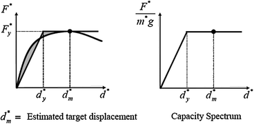

  

  Linearization of capacity curve

• 10. Determination of the period of the equivalent single degree of freedom system T* as:

  $$ {\text{T}}^{ * } = 2\pi \sqrt {\frac{{{\text{m}}^{ * } {\text{d}}_{\text{y}}^{ * } }}{{{\text{F}}_{\text{y}}^{ * } }}} $$

  (5)

• 11. Determination of the target displacement for the equivalent single degree of freedom system as:

  $$ {\text{d}}_{\text{et}}^{ * } = {\text{S}}_{\text{e}} ( {\text{T}}^{ * } )\left( {\frac{{{\text{T}}^{ * } }}{{ 2\uppi}}} \right)^{ 2} $$

  (6)

  where S_e(T*) is the elastic acceleration response spectrum at the period T*. For the determination of the target displacement $d_{t}^{ * }$ for structures in the short period range and for structures in the medium and long period ranges, different expressions should be used.

  • (a) T^* < T_C (short period range)

    • If ${\text{F}}_{\text{y}}^{ * } / {\text{m}}^{ * } \ge {\text{S}}_{\text{e}} ( {\text{T}}^{ * } )$, the response is elastic and thus:

      $$ {\text{d}}_{\text{t}}^{ *} {\text{ = d}}_{\text{et}}^{ *} $$

      (7)

    • If ${\text{F}}_{\text{y}}^{ *} / {\text{m}}^{ *} \;{ < }\;{\text{S}}_{\text{e}} ( {\text{T}}^{ *} )$, the response is nonlinear and:

      $$ \begin{aligned} {\text{d}}_{\text{t}}^{ *} = & \frac{{{\text{d}}_{\text{et}}^{ *} }}{{{\text{q}}_{\text{u}} }}\left( { 1+ \left( {{\text{q}}_{\text{u}} - 1} \right)\frac{{{\text{T}}_{\text{C}} }}{{{\text{T}}^{ *} }}} \right) \ge {\text{d}}_{\text{et}}^{ *} \\ & {\text{with}}\quad {\text{q}}_{\text{u}} = \frac{{{\text{S}}_{\text{e}} ( {\text{T}}^{ *} ) {\text{m}}^{ *} }}{{{\text{F}}_{\text{y}}^{ *} }} \\ \end{aligned} $$

      (8)

      where q_u is the ratio between the acceleration in the structure with unlimited elastic behavior S_e(T*) and in the structure with limited strength ${\rm F}_{y}^{*} /{\rm m}^{*}$.

  • (b) T^* ≥ T_C (medium and long period range), the response is nonlinear and:

    $$ {\text{d}}_{\text{t}}^{*} = {\text{d}}_{\text{et}}^{*} \quad {\text{with}}\quad {\text{d}}_{\text{t}}^{*} \le 3\,{\text{d}}_{\text{et}}^{*} $$

    (9)

• 12. The target displacement of the multi degree of freedom system is then:

  $$ {\text{d}}_{\text{t}} =\Gamma {\text{d}}_{\text{t}}^{ *} $$

  (10)

2 Case Study

The building is eight (08) stories with regularity in plan and elevation. The structure is reinforced concrete resisting moment frames with hollow clay bricks infill walls. A configuration of four (04) longitudinal bays, two (02) transversal bays is considered in this study. Typical columns height in this study are selected as 3.40 m, except for the first floor 4.45 m. The building is located in a high seismic zone (Zone III) with administrative usage (BAEL 91 1999). The details of beams and columns are shown in Table 1.

• The grade of concrete is f_c28 = 20 MPa.

• The grade of steel is f_e = 235 MPa.

• The roof dead load is GT = 6.53 KN/m².

• The roof live load is QT = 1 KN/m².

• The current level dead load is GE = 5.51 KN/m².

• The current level live load is QE = 2.5 KN/m².

Figure 2 shows 3D model of the structure using ETABS program (ETABS 2013).

Table 1. Dimensions of beams and columns

Fig. 2.

Structure model in 3D

3 Results

3.1 Linear Static Analysis

The main intrinsic characteristic of the structure in terms of natural periods and mode shapes are summarized in Tables 2 and 3. Table 4 shows the results of absolute displacements using the response spectrum method considering twenty four (24) for the two main longitudinal (XX) and transversal (YY) directions.

Table 2. Natural periods and modal participating mass ratios

Table 3. Mode shapes for the two first modes

Table 4. Absolute displacements with LRSM

3.2 Nonlinear Static Analysis

The nonlinear static analysis using pushover method gave the capacity curves for the main longitudinal (XX) and transversal (YY) directions as shown in Figs. 3 and 4.

Fig. 3.

Capacity curve for (XX) direction

Fig. 4.

Capacity curve for (YY) direction

The modal participation factors of the first natural modes for the main transversal (XX) and transversal (YY) directions are shown in Table 5.

Table 5. Modal participation factors

The main parameters of the equivalent single degree of freedom are shown in Table 6.

Table 6. Main parameters of equivalent SDOF system

The nonlinear static analysis using pushover method gave the absolute displacements for the two main longitudinal (XX) and transversal (YY) directions as shown in Table 7.

Table 7. Absolute displacements with NLSA

The main results in terms of absolute displacements with the elastic and non elastic analysis are shown in Figs. 5 and 6.

Fig. 5.

Absolute displacements for (XX) direction

Fig. 6.

Absolute displacements for (YY) direction

4 Discussion

• The linear analysis with linear spectrum method in terms of absolute displacements showed that the demand is less than the capacity for the longitudinal direction (XX).

• The linear analysis with linear spectrum method in terms of absolute displacements showed that the demand is greater than the capacity for the transversal direction (YY).

• The nonlinear analysis with pushover analysis in terms of absolute displacements showed that the demand is greater than the capacity for both longitudinal (XX) and transversal (YY) directions.

• Even though all the modes were considered in the linear analysis, the results showed a great difference compared to the nonlinear analysis.

• The nonlinear static analysis showed that the obtained values of absolute displacements are more than double than those obtained for the linear static analysis.

• For adjacent buildings, the dimension of the seismic joint is a critical choice. In case of a small gap, the hammering effect could be dangerous. Otherwise, in case of a large gap, it’s not economic.

5 Conclusion

The analysis of absolute displacements of a building using linear response spectrum methods, taking into account indirectly the nonlinear behavior of structural elements by introducing the behavior factor, and the nonlinear static analysis using pushover procedure have been performed. The results showed a large difference between the two methods. The question remains, is the response spectrum response more conservative, or the nonlinear static analysis less conservative?

One can say that the type of loading in the nonlinear static analysis has a predominant role to determine the capacity curve.

References

DTR BC 48: Règles Parasismiques Algériennes, RPA99/Version 2003. Centre National Recherche Appliquée En Génie Parasismique (CGS), Algérie (2003)
Iqbal, S.: Performance Based Design Modeling for Pushover Analysis Use of the Pushover Curve. Computers and Structures. University of Berkley, California (1999)
Mouroux, P., Negulescu, C.: Comparaison pratique entre les méthodes déplacement de l’ATC 40 (en amortissement) et de l’Eurocode 8 (en ductilité). 7ème Colloque National AFPS 2007, Ecole Centrale Paris (2007)
Poursha, M., et al.: Assessment of conventional nonlinear static procedures with FEMA load distributions and modal pushover analysis for high-rise buildings. Int. J. Civil Eng. 6(2), 142–157 (2008)
CEN Eurocode 8: Design provisions for earthquake resistance of structures. Part 1.1: General rules - seismic actions and general requirements for structures (2003)
BAEL 91: Technical rules of conception and design of constructions in reinforced concrete according to limit states. BAEL 91 revised 99 (1999)
ETABS 13: CSI analysis reference manual. Computers and structure. University of Berkeley, California (2013)
Author information
Authors and Affiliations
Corresponding author
Editor information
Editors and Affiliations
Rights and permissions
Copyright information
© 2018 Springer International Publishing AG
About this paper
Cite this paper
Youcef, M., Abderrahmane, K., Benazouz, C. (2018). Seismic Performance of RC Building Using Spectrum Response and Pushover Analyses. In: Rodrigues, H., Elnashai, A., Calvi, G. (eds) Facing the Challenges in Structural Engineering. GeoMEast 2017. Sustainable Civil Infrastructures. Springer, Cham. https://doi.org/10.1007/978-3-319-61914-9_13
Download citation
DOI: https://doi.org/10.1007/978-3-319-61914-9_13
Published:
Publisher Name: Springer, Cham
Print ISBN: 978-3-319-61913-2
Online ISBN: 978-3-319-61914-9
eBook Packages: Earth and Environmental ScienceEarth and Environmental Science (R0)