Equations of Motion

Abstract

Simulation of a physical system means to calculate the time evolution of a model system in many cases. We consider a large class of models which can be described by a first order initial value problem for the state vector Y (possibly of very high dimension) which contains all information about the system. Our goal is to calculate the time evolution of the state vector numerically. For obvious reasons this can be done only for a finite number of time values and we have to introduce a grid of discrete times which for simplicity are assumed to be equally spaced. Advancing time by one step formally involves the calculation of an integral which can be a formidable task since the integrand depends on time via the time dependence of all the elements of the state vector. In this chapter we discuss several strategies for the time integration. The explicit Euler forward difference has low error order but is useful as a predictor step for implicit methods. A symmetric difference quotient is much more accurate. It can be used as the corrector step in combination with an explicit Euler predictor step and is often used for the time integration of partial differential equations. Methods with higher error order can be obtained from a Taylor series expansion, like the Nordsieck and Gear predictor-corrector methods which have been often applied in molecular dynamics calculations. Runge–Kutta methods are very important for ordinary differential equations. They are robust and allow an adaptive control of the step size. Very accurate results can be obtained for ordinary differential equations with extrapolation methods like the famous Gragg-Bulirsch-Stoer method. If the solution is smooth enough, multistep methods are applicable, which use information from several points. Most known are Adams-Bashforth–Moulton methods and Gear methods (also known as backward differentiation methods), which are especially useful for stiff problems. The class of Verlet methods has been developed for molecular dynamics calculations. They are symplectic and time reversible and conserve energy over long trajectories.

Problems

Problem 13.1 Circular Orbits

In this computer experiment we consider a mass point moving in a central field. The equation of motion can be written as the following system of first order equations:

(13.170)

For initial values

$$\begin{aligned} \left( \begin{array}{c} x\\ y\\ v_{x}\\ v_{y} \end{array}\right) =\left( \begin{array}{c} 1\\ 0\\ 0\\ 1 \end{array}\right) \end{aligned}$$

(13.171)

the exact solution is given by

$$\begin{aligned} x=\cos t\quad y=\sin t. \end{aligned}$$

(13.172)

The following methods are used to calculate the position x(t), y(t) and the energy

$$\begin{aligned} E_{tot}=E_{kin}+E_{pot}=\frac{1}{2}(v_{x}^{2}+v_{y}^{2})-\frac{1}{\sqrt{x^{2}+y^{2}}}. \end{aligned}$$

(13.173)

• The explicit Euler method (13.3)

$$\begin{aligned} \begin{array}{c} x(t_{n+1})=x(t_{n})+v_{x}(t_{n})\varDelta t\\ y(t_{n+1})=y(t_{n})+v_{y}(t_{n})\varDelta t\\ v_{x}(t_{n+1})=v_{x}(t_{n})-\frac{x(t_{n})}{R(t_{n})^{3}}\varDelta t\\ v_{y}(t_{n+1})=v_{y}(t_{n})-\frac{y(t_{n})}{R(t_{n})^{3}}\varDelta t. \end{array} \end{aligned}$$

(13.174)

• The 2nd order Runge–Kutta method (13.7.1)

which consists of the predictor step

$$\begin{aligned} x(t_{n}+\varDelta t/2)=x(t_{n})+\frac{\varDelta t}{2}v_{x}(t_{n}) \end{aligned}$$

(13.175)

$$\begin{aligned} y(t_{n}+\varDelta t/2)=y(t_{n})+\frac{\varDelta t}{2}v_{y}(t_{n}) \end{aligned}$$

(13.176)

$$\begin{aligned} v_{x}(t_{n}+\varDelta t/2)=v_{x}(t_{n})-\frac{\varDelta t}{2}\frac{x(t_{n})}{R(t_{n})^{3}} \end{aligned}$$

(13.177)

$$\begin{aligned} v_{y}(t_{n}+\varDelta t/2)=v_{y}(t_{n})-\frac{\varDelta t}{2}\frac{y(t_{n})}{R(t_{n})^{3}} \end{aligned}$$

(13.178)

and the corrector step

$$\begin{aligned} x(t_{n+1})=x(t_{n})+\varDelta t\, v_{x}(t_{n}+\varDelta t/2) \end{aligned}$$

(13.179)

$$\begin{aligned} y(t_{n+1})=y(t_{n})+\varDelta t\, v_{y}(t_{n}+\varDelta t/2) \end{aligned}$$

(13.180)

$$\begin{aligned} v_{x}(t_{n+1})=v_{x}(t_{n})-\varDelta t\frac{x(t_{n}+\varDelta t/2)}{R^{3}(t_{n}+\varDelta t/2)} \end{aligned}$$

(13.181)

$$\begin{aligned} v_{y}(t_{n+1})=v_{y}(t_{n})-\varDelta t\frac{y(t_{n}+\varDelta t/2)}{R^{3}(t_{n}+\varDelta t/2)}. \end{aligned}$$

(13.182)

• The fourth order Runge–Kutta method (13.7.3)

• The Verlet method (13.11.5)

$$\begin{aligned} x(t_{n+1})=x(t_{n})+\left( x(t_{n})-x(t_{n-1})\right) -\varDelta t\frac{x(t_{n})}{R^{3}(t_{n})} \end{aligned}$$

(13.183)

$$\begin{aligned} y(t_{n+1})=y(t_{n})+\left( y(t_{n})-y(t_{n-1})\right) -\varDelta t\frac{y(t_{n})}{R^{3}(t_{n})} \end{aligned}$$

(13.184)

$$\begin{aligned} v_{x}(t_{n})=\frac{x(t_{n+1})-x(t_{n-1})}{2\varDelta t}=\frac{x(t_{n})-x(t_{n-1})}{\varDelta t}-\frac{\varDelta t}{2}\frac{x(t_{n})}{R^{3}(t_{n})} \end{aligned}$$

(13.185)

$$\begin{aligned} v_{y}(t_{n})=\frac{y(t_{n+1})-y(t_{n-1})}{2\varDelta t}=\frac{y(t_{n})-y(t_{n-1})}{\varDelta t}-\frac{\varDelta t}{2}\frac{y(t_{n})}{R^{3}(t_{n})}. \end{aligned}$$

(13.186)

To start the Verlet method we need additional coordinates at time $-\varDelta t$ which can be chosen from the exact solution or from the approximation

$$\begin{aligned} x(t_{-1})=x(t_{0})-\varDelta t\, v_{x}(t_{0})-\frac{\varDelta t^{2}}{2}\frac{x(t_{0})}{R^{3}(t_{0})} \end{aligned}$$

(13.187)

$$\begin{aligned} y(t_{-1})=y(t_{0})-\varDelta t\, v_{y}(t_{0})-\frac{\varDelta t^{2}}{2}\frac{y(t_{0})}{R^{3}(t_{0})}. \end{aligned}$$

(13.188)

• The leapfrog method (13.11.8)

  

  (13.189)
  

  (13.190)
  

  (13.191)
  

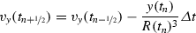  (13.192)

where the velocity at time $t_{n}$ is calculated from

(13.193)

(13.194)

To start the leapfrog method we need the velocity at time which can be taken from the exact solution or from

(13.195)

(13.196)

Compare the conservation of energy for the different methods as a function of the time step $\varDelta t$. Study the influence of the initial values for leapfrog and Verlet methods.

Problem 13.2 N-body System

In this computer experiment we simulate the motion of three mass points under the influence of gravity. Initial coordinates and velocities as well as the masses can be varied. The equations of motion are solved with the 4th order Runge–Kutta method with quality control for different step sizes. The local integration error is estimated using the step doubling method. Try to simulate a planet with a moon moving round a sun!

Problem 13.3 Adams-Bashforth Method

In this computer experiment we simulate a circular orbit with the Adams-Bashforth method of order $2\ldots 7$. The absolute error at time T

$$\begin{aligned} \varDelta (T)=|x(T)-\cos (T)|+|y(t)-\sin (T)|+|v_{x}(T)+\sin (T)|+|v_{y}(T)-\cos (T)| \end{aligned}$$

(13.197)

is shown as a function of the time step $\varDelta t$ in a log-log plot. From the slope

$$\begin{aligned} s=\frac{d(\log _{10}(\varDelta ))}{d(\log _{10}(\varDelta t))} \end{aligned}$$

(13.198)

the leading error order s can be determined. For very small step sizes rounding errors become dominating which leads to an increase $\varDelta \sim (\varDelta t)^{-1}$.

Determine maximum precision and optimal step size for different orders of the method. Compare with the explicit Euler method.