Linking Manufacturing Cells

Abstract

In Chap. 5 we have developed the concept of multi-product, also called mixed-product, manufacturing cell, to maximize cell utilization and to increase at the same time the flexibility of a self-controlled manufacturing unit enouncing the following theorems:

• Theorem of Generalized Throughput

• Theorem of Lean Batch Sizing

• Theorem of Cell Product Congruency

• Theorem of Vulnerability of Mono-product Cell.

In Chap. 5 we have developed the concept of multi-product, also called mixed-product, manufacturing cell, to maximize cell utilization and to increase at the same time the flexibility of a self-controlled manufacturing unit enouncing the following theorems:

• Theorem of Generalized Throughput

• Theorem of Lean Batch Sizing

• Theorem of Cell Product Congruency

• Theorem of Vulnerability of Mono-product Cell.

In the following sections we will develop the concepts of the third level of manufacturing complexity according to the TPS model of Fig. 2.3 dealing with linking different manufacturing cells, i.e. a complex multi-cell manufacturing environment or conveying the components of different asynchronous cells to a main manufacturing transfer line. We will see the concept of a supermarket linking the decoupled supply to demand as well as the concept of synchronous and asynchronous manufacturing lines and how a milk-run optimizes the utilization of a centralized supermarket. We will explain the paradigm change from queuing theory dominated push systems to downstream controlled replenishment theory of Lean pull systems with JIT philosophy.

6.1 The Paradigm Change: From Push to Pull

Independent of the production principle, i.e. make-to-stock or make-to-order, Western production philosophy has been characterized mainly by the push manufacturing principle governed by complex computer-assisted MRP and later ERP systems; the consequence is to push batches through different workstations according to the scheduled routing. The formation of WIP, i.e. queued orders between the workstations according to equation system (3.7), is the consequence. The WIP between the workstations usually is not controlled and depends on the cycle times of the operations. This becomes the potential playground of Lean improvement or remains the typical application domain of queuing theory. Before performing push-pull manufacturing principles and e.g. EDD scheduling or similar principles, FIFO scheduling principle with B&Q transfer principle has been the reality in western manufacturing plants.

In the Japanese production philosophy, namely the TPS, manufacturing cells are linked via supermarkets as soon as the cycle times of the cells are different. A supermarket can also be seen as a kind of WIP (if it is not the FGI) but the origin is completely different and it fulfills a functional task of interfacing demand and supply, i.e. to separate the supply loop from the demand, two loops with different governing logics.

The control of both manufacturing principles is shown in Fig. 6.1 with the help of hydraulic modeling already introduced with Fig. 2.4 showing exemplarily the control of a water reservoir. The push principle has no explicit control once the production is launched; the control of course exists, but it is only on the ERP level of production planning, i.e. a contingent managerial one-off decision. The simple causal model and the relative representation with VSM symbols is shown in Fig. 6.2. The left side shows two possible interventions: the more WIP is forming the more the production scheduling manager tries to increase production to reduce the WIP; investments might be the consequences, or the planning department will reduce order release to the shopfloor, but with the consequence that the order backlog will grow. The contrary is the pull principle shown in Fig. 6.3 which represents a self-controlled unit.

Fig. 6.1

Comparison of Push and Pull manufacturing principles with the help of the hydraulic model

Fig. 6.2

Push principle with sporadic non-systemic control by upstream (primary approach “make-all-what-you-can”)

Fig. 6.3

Pull principle controlled by downstream (reactive approach “make-only-what-is-needed”)

The self-controlled production-cell unit follows in principle a make-to-stock philosophy. However, the stock is not a just-in-case stock created by the consequence of a push principle but a stock with decoupling function of the downstream from the upstream operation. It serves to implement, or even better, it represents the JIT pull manufacturing principle. The call-offs can be served immediately by the small quantity available in the supermarket and the supermarket decoupling stock is replenished as soon as the Kanban (Japanese for signal) is given by the system’s status itself. On the other hand, with the push principle orders have to be scheduled and represent the backlog with backlog waiting time BWT. The constant T of λ = 1/T in Fig. 6.1 is the “mean adaptation time”, which inverse value in production represents the capacity, i.e. the exit rate ER where T is the cycle time CT. The y level is controlled by the K_max setting which represents the maximum level of the supermarket. How to calculate the K_max will be shown in Chap. 7. We can summarize this section by saying: pull manufacturing principles are demand triggered and therefore takt rate TR-controlled, whereas push manufacturing principles are scheduling input rate and are therefore IR-governed. These are two opposite manufacturing philosophies.

In the nineteen-eighties, the conceptual difference between push and pull manufacturing principle was hardly understood in Western enterprises leading to incomprehension and has been provoking a still ongoing debate not only in production planning departments, if ever. Indeed, Western production systems of SME are still largely dominated by a push manufacturing principle, being pull principle against Western natural production logic. This has been reflected in the optimization of MRP systems, development, which has been leading finally to today’s ERP systems.

6.2 Supermarkets

The concept of supermarkets and their replenishment are not a Toyota invention, but have been first implemented in America during the nineteen-forties. It is told, Taiichi Ohno had been inspired by this demand pull governed replenishment of commercial supermarkets and transferred the concept to its automotive industry. Supermarkets have to be understood as the “availability from shelf” of a large variety but of limited quantity of products which are replenished as soon as they are taken out of the supermarket.

Contrary to retail supermarkets, industry supermarkets are usually installed for high runner products, where the availability has to be immediate but cannot be produced to the consumption speed requested by the customer (see also Sect. 7.1 and Fig. 7.1). Supermarkets are implemented to avoid the consequence of classic ERP planning systems with deterministic, i.e. scheduled queuing systems. Supermarkets help to install self-controlled systems, which in fact are manufacturing cells with pitch-scheduled replenishment (i.e. in small batches) according to a random demand, i.e. either stochastically or deterministically governed call-offs.

Let us calculate exemplarily the dynamic behavior of the supermarket stock level according to the hydraulic model of Fig. 2.4, but now applied to the system shown on the right side of Fig. 6.1 with a Kanban controlled level of K_max = y_K and translated to causal system dynamics as well as VSM notation of Fig. 6.3. The differential equation of first order describing the system is

$$ \begin{array}{c}\hfill \frac{dy}{dt}={q}_{\mathit{\mathrm{in}}}-{q}_{\mathit{\mathrm{out}}}=q(y)-q(t)\hfill \\ {}\hfill \dot{y}=\lambda \cdot \left({y}_K-y\right)-q(t)\hfill \\ {}\hfill \dot{y}\cdot {e}^{\lambda t}+\lambda y\cdot {e}^{\lambda t}=\lambda {y}_K\cdot {e}^{\lambda t}-q(t)\cdot {e}^{\lambda t}=\frac{d}{dt}\left(y\cdot {e}^{\lambda t}\right)\hfill \\ {}\hfill y\cdot {e}^{\lambda t}-{y}_0=\lambda {y}_k\underset{0}{\overset{t}{\int }}{e}^{\lambda \tau} d\tau -\underset{0}{\overset{t}{\int }}q\left(\tau \right){e}^{\lambda \tau} d\tau \hfill \\ {}\hfill y\cdot {e}^{\lambda t}-{y}_0=\lambda {y}_k{\left[\frac{1}{\lambda }{e}^{\lambda \tau}\right]}_0^t-\underset{0}{\overset{t}{\int }}q\left(\tau \right){e}^{\lambda \tau} d\tau \hfill \\ {}\hfill y\cdot {e}^{\lambda t}-{y}_0={y}_k\left({e}^{\lambda t}-1\right)-\underset{0}{\overset{t}{\int }}q\left(\tau \right){e}^{\lambda \tau} d\tau \hfill \\ {}\hfill y-{y}_0\cdot {e}^{-\lambda t}={y}_k\left({e}^{\lambda t}-1\right)\cdot {e}^{-\lambda t}-{e}^{-\lambda t}\cdot \underset{0}{\overset{t}{\int }}q\left(\tau \right){e}^{\lambda \tau} d\tau \hfill \\ {}\hfill y(t)={y}_0{e}^{-\lambda t}+{y}_K\left(1-{e}^{-\lambda t}\right)-{e}^{-\lambda t}\underset{0}{\overset{t}{\int }}q\left(\tau \right){e}^{\lambda \tau} d\tau \hfill \end{array} $$

(6.1)

and after transforming when we set the expression

$$ {y}_K-{e}^{-\lambda t}\left({y}_K-{y}_0\right)= C $$

we observe the expected results that

$$ \underset{t\to {0}^{+}}{ \lim } C={y}_0 $$

$$ \underset{t\to \infty }{ \lim } C={y}_K $$

Now according to the time-depending outflow function q(τ) of Eq. (6.1) there exist different cases. E.g. for q(t) = q₀ i.e. a constant outflow, where in our case q₀ < y_K we can set

$$ q\left( t,{t}_0\right)={q}_0\cdot F\left( t-{t}_0\right) $$

and defining the step function F(t − t₀) for t > 0 which assumes the values for

$$ t-{t}_0<0\to F\left(t-{t}_0\right)=0 $$

$$ t-{t}_0\ge 0\to F\left(t-{t}_0\right)=1 $$

Equation (6.1) becomes better readable

$$ \begin{array}{l}\begin{array}{c}\hfill y=C-{e}^{-\lambda t}\cdot {q}_0\underset{0}{\overset{t}{\int }}F\left(\tau -{t}_0\right)\cdot {e}^{\lambda \tau} d\tau \hfill \\ {}\hfill y=C-{e}^{-\lambda t}{q}_0F\left(t-{t}_0\right)\cdot \frac{1}{\lambda}\left({e}^{\lambda t}-{e}^{\lambda {t}_0}\right)\hfill \\ {}\hfill y=C-\frac{q_0}{\lambda }F\left(t-{t}_0\right)\cdot \left(1-{e}^{\lambda \left({t}_0-t\right)}\right)\hfill \\ {}\hfill y=C-\frac{q_0}{\lambda }F\left(t-{t}_0\right)\cdot \left(1-\frac{1}{e^{\lambda \left(t-{t}_0\right)}}\right)\hfill \\ {}\hfill \underset{t\to \infty }{ \lim }y={y}_K-\frac{q_0}{\lambda}\hfill \end{array}\\ {}\end{array} $$

(6.2)

Equation (6.2) represents the stable level of the supermarket, i.e. the maximum level of the supermarket has to be sized greater than q₀T. In reality, the outflow will not have a continuous nature. Therefore, let us try to model the more realistic case for a production environment with a time-discrete outflow.

Again, to do so, we will take the most common case for a discrete call-off type of demand in which q(τ) is a succession of impulsive functions q(t) of Diraq’s δ-function applied for t=t_i (where i=0, 1, ..., n), where a single impulsive function is

$$ q(t)=\delta \left( t,{t}_0\right)\cdot {Q}_0 $$

with $\underset{t_b\to {t}_0^{+}}{\underset{t_a\to {t}_0^{-}}{ \lim }}\underset{t_a}{\overset{t_b}{\int }}\delta \left(\tau, {t}_0\right)\cdot d\tau =1$

i.e. for a succession we get $q(t)=\sum_{i=0}^n\delta \left( t,{t}_i\right)\cdot {Q}_i$

The Equation (6.1) $y={y}_0{e}^{-\lambda t}+{y}_K\left(1-{e}^{-\lambda t}\right)-{e}^{-\lambda t}\underset{0}{\overset{t}{\int }} q\left(\tau \right){e}^{\lambda \tau} d\tau$ becomes

$$ y= C-{e}^{-\lambda t}\cdot \sum_{i=0}^n\frac{Q_i\cdot F\left( t-{t}_i\right)}{e^{-\lambda {t}_i}} $$

where F(t − t_i) are the unitary step functions becoming active for t > t_i cumulating and remaining then constant. Please note, the replenishment is still shown as a continuous function, but will most likely happen in the quantity of the pitch. For the time t > t_n

$$ y={y}_K- Y\cdot {e}^{-\lambda t} $$

where $Y=\left({y}_K-{y}_0\right)-\sum_{i=0}^n\frac{Q_i}{e^{-\lambda {t}_i}}$

showing the stepwise character for every instant t_i with the quantity Q_i.

We have assumed in the left figure of 6.3, that no delay exists to put the manufactured products into stock; this corresponds of course not to reality. As we know in the meanwhile, this has to be as short as possible following the MLT_nPF law. Let us therefore describe a more realistic model of the system dynamics regarding our manufacturing cell which is represented in Fig. 6.4. Nota bene, in reality, for a mixed-product cell the Heijunka box introduces itself an additional BWT as small as it may be, but known in advance and buffered by the supermarket.

Fig. 6.4

Complete system dynamics model of a cell taking manufacturing delay into consideration

Manufacturing creates necessarily a WIP, which by its turn entails a delivery delay to stock; in this case it is the “white box” WIP of the usually considered “black box” manufacturing cell on the high level VSM modeling. Although the WIP might be minimal for SPF, the cycle times of the operations within the cell and the difference between the reorder and the manufacturing rate entails, that there will be a delay from the time of ordering, i.e. the Kanban signalizing to begin production, until the pieces are stocked into the Kanban supermarket represented by the MLT of the batch. This shows the importance of the MLT concept compared to the usually applied PLT; indeed, the discrete time interval (t_i+1 − t_i) of integration has to be choosen appropriately to have no indesired unstable solution generated by the computational procedure and not by the system's characteristics. Here the model shows the take-out of the material of the RMI with the T_r cycle time. The equations governing this system are becoming more complex leading to differential equations of second order with exponential smoothing sinusoidal development. We will maintain our promise to limit math and refer to simulation packages e.g. [1, 2].

Due to the fact that we are ideally in a SPF regime, the reorder rate, i.e. the outflow from the raw material inventory RMI, and the stocking rate, i.e. the WIP being transferred at the end to the Kanban inventory, are proportional. Differential equations allow to calculating analytically the evolution of the stock level. In reality, due to the necessary high effort, such systems are not calculated via solving of differential equations, but the behavior of such self-regulated systems is explored via the help of discrete simulations applying a stepwise computational approach [1, 2].

The attentive reader might have noticed that the approach of differential equation aggregates the reality of single discrete events, such as a decision to replenish a Kanban-governed inventory, into a continuous succession of actions. Indeed, the difference (y_K − y) is evaluated in each infinitesimal instant dt, or Δt in the case of discrete simulation, and has therefore an exponential asymptotic filling approach, which in reality is not the case applying the reordering only when reaching the reorder level, following then a stepwise (according to the MLT one-batch law) or linear (according to the PLT single piece law) stock filling approach. The T_r corresponds in reality to the PIT and the T_s corresponds to the inverse of the ER of the cell and the exiting of the RMI stock has forcedly to be equal to the ER of the cell. Nevertheless, this idealization does not represent a concern when the system to be modeled is complex. Further, this does not mean, that discrete decision events for replenishment cannot be taken explicitly into account, as we have just seen for the outflow. We will not go further into this matter and refer to commercial discrete simulation packages [1, 2]. Nevertheless, we want to pinpoint, in order not to have an undesired strange behavior of the system's dynamic under evaluation, the discrete time step Δt in all from DYNAMO derived compiler types, have to be chosen appropriately, which in fact should be smaller than the smallest delay. For dynamic discrete simulation we refer to generally applicable DYNAMO-derived simulation packages such as e.g. STELLA e.g. [2] or more dedicated to manufacturing, consult e.g. [1].

Lemma of Supermarket Replenishment (or Lemma of Product Availability)

The replenishment of a supermarket from a mixed-product manufacturing cell has to be conceived in that way, that all products of the supermarket are readily available by storing the minimum sustainable K_max quantity, i.e. the Corollary to the Theorem of Lean Batch Sizing (Corollary of CT of a Mixed-product Workstation) applies.

In Sect. 7.3, How to seize a replenishment Kanban, we will take in consideration the delay to produce the reordered parts with a common arithmetic calculation approach to define the y_K representing the Kanban “maxloop”, i.e. the number of Kanbans in the system.

Let us now be more practical and respond to the question where to install, i.e. to locate a supermarket. We can distinguish two main location principles:

• shared generic supermarket: one or more centralized supermarkets with milk-run conveying to the POU (point-of-use); the centralized supermarket needs a dichotomic Kanban system which distinguishes first a withdrawal Kanban (i.e. signaling the consumption of products from the central supermarket) and second a production Kanban (i.e. the order to replenish the central supermarket with products)

• specific POU supermarket: several decentralized supermarkets located in between the upstream and downstream adjacent cells as shown in Fig. 5.7 and Fig. 6.5, i.e. adjacent to the POU; here the Kanban device is unique but with different possible implementing techniques depending from the contingent characteristic of the operation: visual (also called triangle Kanban) usually applied for batches with technical restriction (e.g. large 30 ton casting units) and patterned scheduling (i.e. rolling aluminium coils from wide to narrow), or cards representing products (e.g. the pack-out quantity) to be produced, usually combined with a Kanban gage (green, white, red colored grid). For practical implementation suggestions consult e.g. [3].

  Fig. 6.5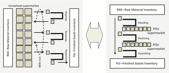

  

  Location principles of centralized supermarket serving POU with milk-run technique versus decentralized supermarkets located at the POU

The decentralized supermarkets allow better to attribute and make the WIP visible and therefore to reduce it further. In addition, time wasted for storing and taking-out the material has to be accounted. Of course, the supply of standard consumption parts at the POU may be supplied from a centralized supermarket with the milk-run. The centralized supermarket and associated milk-run can be implemented via AGV (automated guided vehicles); this eliminates the Muda associated to the operator distributing the required products and collecting the Kanban cards at the Kanban post. In this cases also random managed and computer controlled storing is possible and makes this option viable (we will not deepen here the topic of different central supermarket storage principles, such as e.g. random storage, affinity storage, frequent use storage principles). The AGV distribution of raw material and components, as well as small consumables to the POU, makes sense and has not to be confounded with the Industry 4.0 intention to let the products, e.g. transported cars, address autonomously distributed working cells; the AGV-distributed material can be performed in parallel to the production, the cars transported via AGV will generate waste in transportation, delaying PLT, a cardinal conception mistake in the case of high performance manufacturing lines [4]. For practical implementation consult e.g. [5].

Which location principle is finally applied, i.e. centralized (shared) or decentralized (specific to POU), is subject to contingent considerations; no general rule can be enounced. Pros and cons have to be established according to cost, i.e. seize/space or logistics/traffic, or simple convenience criteria.

6.3 Synchronous and Asynchronous Lines

To assemble a finished or intermediate product following the assembly scheme from different components according to the BOM (bill of material), different approaches are possible. In western production plants the predominant approach has been the time-synchronous assembly type. This approach is characterized by the simultaneous arrival of the different parts components to the assembly area. To assure the time-concomitant presence of all necessary parts, more or less sophisticated planning tools are used, such as CPM (critical path method), PERT (program evaluation and review technique) or even Petri net modeling. If a component experiences a delay, the assembly cannot start and the already available parts will congest the assembly area until all necessary parts are present, necessitating at the limit preemption, and a change of the scheduling priority causing delay in punctual delivery. It is obvious, that the main transfer principle applied is the push B&Q, although the assembly operation itself then might be organized within a SPF line.

On the other hand, supermarkets allow an asynchronous approach, such as depicted in Fig. 6.6, where both assembly principles are shown, i.e. the

• synchronous assembly principle, and

• asynchronous assembly principle.

Fig. 6.6

Assembly principles of synchronous versus asynchronous assembly lines

In the asynchronous assembly principle the replenishment of the components supermarkets are self-controlled and based on demand-pull from the downstream assembly operation. This allows a higher flexibility of the production mix, always within a certain predefined scope of course, but is ideal to implement the JIT concept. On the other hand, mainly in Western automotive industry the just-in-sequence (JIS) is returning, which corresponds to a synchronous assembly principle, necessitating ERP systems. Toyota implemented JIS-synchronized lines feeding the final assembly TFL.

In the case of asynchronous lines, e.g. on large scale transfer lines (TFL), only the sequence of the TFL has to be scheduled (Fig. 6.7); the cells feeding the backbone assembly line will be Kanban-scheduled according to the withdrawal of the components from the small supermarket interfacing assembly. Therefore it is the backbone TFL which determines the necessary sub-component to be assembled to the product, sub-components which are ready to be extracted from the supermarkets along the line. This allows also a last minute change of the configuration of the product. The sometimes applied just-in-sequence (JIS) principle of the components, e.g. German car manufacturer BMW, sequence necessarily transmitted to the tier 1 OEM components manufacturer by the automotive manufacturer, requires a smaller buffer area, but is locked regarding the scheduling of sequence; in reality it is a step backward regarding TPS flexibility, especially in the case if a defective part is delivered. The JIS might have its reason of existence for high variability of mix, transferring the problems to the tier 1 suppliers. The JIT cells, however, are supplied by a milk-run concept, conveying the required raw material according to the withdrawal Kanban, i.e. the milk-run combines by bringing products to the POU and taking cards from the Kanban post. Note, the frequency of the milk-run needs to be calculated based on number of cells, pitch, time to get the material, and time to dispatch the material to the POU; this exercise is not carried-out in this book.

Fig. 6.7

Asynchronous level-pulled feeding of a central TFL with milk-run supplied mixed-product cells

Certain rolling stock manufacturers are still assembling railway wagons from kits. Today, kit assembly operations (as well as completely knocked-down kits of automotive) are outdated for industrial scale operations. The reason for that is, that a defective part does not allow to completing to assemble the kit and therefore congesting the assembly area until the defective part has been substituted, whereas in asynchronous lines the part is put aside and exchanged by the next part available.

Lemma of Asynchronous Line (or Lemma of Maximum Flexibility)

In operations of assembling sub-components, to guarantee a high flexibility of scheduling, the supermarket's replenishment make-to-stock principle allows to maintain high performance in asynchronous assembly lines, eliminating the need for kit parts synchronization or just-in-sequence scheduling.

6.4 Requirements for JIT Manufacturing

The JIT diction is widely used but not always understood by everybody in the same way, sometimes even confounded with the limited concept of OTD to customers. Commonly, in the original sense, the JIT of TPS is intended that the product is manufactured exactly then when it is needed, i.e. JIT regarding the manufacturing of products within the operations.

JIT, as it has been interpreted by Hall (1983), is equivalent with stockless production leading to zero inventories and WIP, and therefore no delay with queuing. Edwards (1983) described the necessary requirements with the seven zeros: zero defects, zero excess lot size, zero set-up, zero break down, zero handling, zero lead time, zero surging [6].

We can synthesize all the statements by generalization, comprising the customer specific OTD, to the supply-demand relation within a manufacturing line. We can even go further and define now JIT mathematically based on the previously enounced theorems of

• SPF dominance (the transfer principle dimension)

• delay or time-trap (the minimum WIP dimension)

• bottleneck (the capacity dimension)

by defining the necessary and sufficient JIT conditions with the equation system (6.3)

$$ JIT:= \left\{\begin{array}{l} pull(SPF)=\underset{n\to 1}{ \lim }{B}_k(n)\\ {} \min PLT=\underset{CT_i={CT}_{i+1}}{ \min } WIP\\ {} \sup {CT}_i={CT}_b\le TT\end{array}\right. $$

(6.3a–6.3c)

or more exactly with Eq. (6.4), because Eqs. (6.3b) and (6.3c) are the conditional requirements, with Eq. (6.3a) being rather the definition of JIT, i.e.

$$ JIT:= \left\{ pull(SPF)=\underset{n\to 1}{ \lim }{B}_k(n)\left| \min PLT=\underset{CT_i={CT}_{i+1}}{ \min } WIP, \sup {CT}_i={CT}_b\le TT\right.\right\} $$

(6.4)

Different than often postulated and falsely believed, Eq. (6.3a) shows unequivocally that Lean has not the aim to attain batch size B_k = 1, but the transfer unit n = 1 defining a SPF, the batch size being a consequence of the product interval time PIT and TR.

Now, the necessary and sufficient requirements for a JIT-production according to TPS at the most aggregated level, which at the end means also OTD, where OTD can be seen as the special case of JIT philosophy at the end of the supply chain, JIT can be formalized and defined with the compact form as

$$ JIT:= \underset{CT_i={CT}_{i+1}}{ \min}\left\{ WIP\right\}=\underset{n\to 1}{ \lim } pull\left\{{B}_k(n)\right\} $$

(6.5)

Equation (6.5) shows that minimizing WIP, which minimizes PLT, and minimal WIP is conditional to a balanced line which is attained by a pull system of a batch with the handled quantity tending to one, i.e. SPF, means supplying JIT. Equation (6.5) can therefore be enounced as the JIT necessary, but not sufficient, requirement for a stockless production leading to the cardinal Lean Theorem:

Cardinal Theorem of Lean (or JIT Theorem)

Necessary but not sufficient requirement for a JIT production, i.e. the time dimension to implement the Lean vision of the right product, at the right place, at the right time, is to strive for batch size one, intended as transfer unit, i.e. a SPF, to minimize WIP and aiming to have a balanced line.

We prefer to write pull instead of push in Eq. (6.5) to stress that the triggering is originated downward, although the difference of push and pull is vanishing according to the CLTM and Eq. (4.21) when the transfer unit tends to one. Please note, that our shortcut description of Lean given at the end of Sect. 2.2 “Lean is a Kaizen-based JIT production” is in-line with the Cardinal Theorem of Lean. By the way, this definition reflects the dichotomic character of Lean, being on the one hand a continuous improvement philosophy following Deming’s PDCA cycle and on the other hand a best performing waste-less production theory.

6.5 The Central Importance of TR

In Chap. 3 we learned the necessary and sufficient conditions for OTD, in Chap. 4 we learned about queuing law and lead time calculation, and in Chap. 5 all about optimal Lean batch sizing. Now let us have a look at how the synthesized math of a manufacturing cell works in order to satisfy OTD. Figure 6.8 summarizes the previous sections and shows the systemic relations between the main variables of a manufacturing system to observe OTD. Please note, as we know now, not PLT but MLT has to be confronted to EDT to match the OTD Theorem, embracing the General Production Requirements.

Fig. 6.8

Systemic JIT relations between TR, B_k(n), CT_b, OTD

Figure 6.8 shows the central importance of TR in a Lean manufacturing system to implement JIT. It shows the influence it has on the key variables batch size B_k(n) as well as cycle time at the bottleneck CT_b of the manufacturing cell. These two variables then influence directly the key variables WIP and ER of the queuing law determining PLT. Further it shows how B_k(n) and CT_b determine the CTT of a mixed-product cell in order that the product mix can be delivered on time and how PIT, i.e. the frequency, when product k is manufactured again, is mutually influenced by B_k(n). The goal is to orient every operation within the manufacturing system to the TR in order to manufacture JIT throughout the in-house value-chain. The TR is therefore the sole alignment information necessary to control the whole production, to which every self-directed cell performance needs to be oriented. Of course, due to technological constraints this orientation is not always possible; in any case the CT_b has to be faster than the required average customer TT. Nevertheless, Fig. 6.8 also reveals that PLT cannot be influenced directly but only via the driving variables WIP and ER to satisfy the customer requested EDT. But it also reveals the central attention one has to put on the bottleneck, which can directly be influenced acting on the bottleneck.

Theorem of Lean Production Control (or Takt Rate Synchronization Theorem)

Necessary condition to have a smooth running JIT production is to align every assembly line but also the asynchronous manufacturing cells to the centrally imposed takt rate TR to implement a customer-pull JIT supply regime. The TR becomes the controlling element of the production.

Corollary to the Theorem of Lean Production Control (Corollary of Self-controlled Units)

If the OTD Theorem is not satisfied by the make-to-order principle within the value stream, Kanban controlled supermarkets (make-to-stock principle) have necessarily to interface adjacent cells, which are decentralized governed self-controlled manufacturing units, integrating production by decoupling supply and demand.

Lemma to the Theorem of Lean Production Control (Lemma of Non-prefabrication)

To comply with the Theorem of Lean Production Control, no prefabrication is necessary which would only congest the shopfloor and create Muda. Everything has to be bottleneck, or generally, pacemaker oriented.

This will lead to the Lemma of “Make to X” Production Principle which will be enounced in Chap. 7.