
Abstract
The intersections in the terminal airspace is an potential factor to cause flight conflicts. The possibility of conflict can be reflected directly from air controller intervention degree. Analyzing the controller intervention degree of intersection is a precise and efficient method to locate airspace congestion location in terminal airspace. After analyzing the historical data, improved density clustering method is used to determine the distribution of intersections in terminal airspace. The method of assessing the controller intervention degree is put forward through the statistics on the changes of the flight elements within certain time and range. The experimental results show that this method can obtain the distribution of conflict and controller pressure points in the terminal area, and is quite consistent with reality. The method can provide fast and accurate optimization basis and improvement direction for the airspace planning work.
You have full access to this open access chapter, Download conference paper PDF
Keywords
1 Introduction
Intersection is an important factor increasing workload for controllers, especially in terminal airspace. Controller intervention degree demonstrate the potential conflicts and complexity of airspace which illustrate the workload of air traffic controller directly. Assessment of controller intervention degree is a good method to understand the complexity of local airspace and distribution of congestion points. Currently, the goal of intervention degree assessment is to evaluate the air traffic controller workload. Simulation and modelling are the common used methods. However, those methods are time consuming and simulation software is expensive. This paper introduces a method to evaluate the controller intervention degree on the basis of analyzing the history flight data. According to controller experience in terminal airspace, the direct result of controller intervention is the changes of flight elements (heading, speed, altitude). Surveillance data is collected and analyzed by adopting improved density clustering to dig out the intersections with the help of improved density-based clustering algorithm, the controller intervention degree of intersection is evaluated by detecting the changes of flight elements.
2 Determination of Intersection Distribution Based on Improved Density-Based Clustering
2.1 Problem Description and Introduction of Improved Density-Based Clustering
The basis for aircraft operating in terminal airspace is the flight procedure. However, deviation happens in actual flight because of the conflict resolution. So, the history flight data is mess, huge and uneven density. Some method should be used to identify prevailing traffic flow to obtain the location of intersections. Density clustering algorithm is the ideal way to obtain the prevailing flow and deal with data sample with arbitrary shape. So, we improved the algorithm and used it to get the location of intersections in this paper.
In order to enhance the efficiency of algorithm, improved density clustering algorithms emerged. Among them, shared nearest neighbor clustering algorithm(SNN) is not susceptible to input parameters, but is suitable to use on uniform density data set. As for this problem, improved SNN clustering algorithm is proposed in this paper. Firstly, sub-cluster of each point is generated and the density of each point is calculated. Then, with the help of optimal two-partition method, an density array of the whole data set is sequenced by grouping data with similar density into same category. Each sub-cluster is assigned a density category tag which demonstrate. Finally, SNN algorithm is used in sub dataset with same category tag to generate the average trajectory.
As air traffic surveillance data is used for experiment, one trajectory is composed with many points, each point can be expressed with a vector pi = [x, y, z, v, α, t, t r ], x, y is the latitude and longitude of point p i , z is the altitude, v is ground speed, αis the heading, t is the collecting time of p i , t r is the trajectory number of which pi belongs to.
2.2 Generation of Sub-clusters
Sub-cluster is a set [R] of data points that have a certain similarity relation with a certain data point. Traffic flow is a dataset of points with certain density and direction. So, the sub cluster is defined as a dataset with distance between points is within the certain scope. The similarity of trajectory points is evaluated with Euclidean distance.
Define sub-cluster of pi(C(p i )) as the data set contains points with distance to pi is less than r:
Where p i , p j are trajectory points, x i , y i is the coordinates of p i , x j , y j is the coordinates of p j , n is the number of points.
In order to reduce the amount of computation and improve the efficiency of algorithm, the search space could be limited to calculate the distance between points. Trajectory point vector contains the latitude, longitude and heading, so the research space could be limited in a neighborhood U(p i ) of the point.
Where, S is the trajectory points set, L is the limited scope of neighborhood, which can be determined by the aircraft speed limit and data collection frequency in the terminal area. Under the condition where r is determined, we use L = r.
2.2.1 Density Distribution Array Generation
The sub-clusters are constructed from each data point in the dataset and the density of the sub-clusters is analyzed. For the data points with the same radius r, the number of track points is larger, indicating that the local density of the sub-clusters is larger. On the contrary, if the number of track points of sub-clusters is similar, their density should be basically the same.
Define the sub-cluster tag: Each sub-cluster contains a certain number of data points, recorded as d ps . According to the magnitude of d ps , sub-cluster are divided into s categories \( (s\,{ \in }\,Z^{ + } ) \). For a given category S g , set its density tag as \( Cat_g(1\,\le\,g\,\le\,s) \). For any given sub-cluster \( Cs(p_{i} )(1\,\le\,i\,\le\,n) \) and category S g , where the number of data points contained in \( Cs(p_{i} ) \) is d psi , the density of sub-cluster Cs(p i ) marked as Cat g .
All the sub-clusters is classified into density distribution array C at , which determines the density distribution of the whole data set. It is large possibility to cluster the points with similar density to same cluster. Sub-clusters with similar density are classified as same category of density distribution. How to measure the similarity of the sub-clusters density is a problem to be considered in clustering. the number of categories is small, the density distribution may be assessed incompletely, and the number of categories is too big, the density distribution is too fragmented and the clustering efficiency is low. The optimal two-partition method is used to divide the sub-clusters into appropriate number of categories. First of all, sub-clusters are sequenced by d sp . The optimal two-partition is to subdivide the sub-clusters according to d ps into two parts at once. The minimum total variance is target for each division, and the partitioning is carried out several times. Minimum number of categories is corresponding to overall variance mapping inflection point with the minimum total variance as target is determined (Fig. 1).

Density array generation based on the optimal two-division method
At the beginning of division, the overall variance decreases fast. After reaching to a certain extent, the trend of reducing the overall variance is getting smaller and smaller. When the number of partitions is the same as the number of sub-clusters, the overall variance is zero. According to this law, the reflection point of the function of the category number and overall variance can be determined, and the reflection point is the optimal division.
2.2.2 Clustering of Sub-clustering with Same Density Tag
After marking each sub-cluster the density tag, we can cluster the sub-clusters with similar density using SNN algorithm to get the average trajectory. Sub-clusters with sparse points may be clustered into a large class without considering the direction, which does not happen in reality. So the same density category sub-clusters can be clustered according to direction into several clusters, because it is easy to separate different direction of traffic flows.
Assume ARR[i] is the sub-cluster set with density category is i, ARR[i].P[j] is the center of sub-cluster j with density category is i. The algorithm is as follows:
-
Step1: judge whether ARR[i] is empty, if true, clustering ends, otherwise turn to Step2;
-
Step2: judge whether any cluster set with same density tag is empty, if empty, i = i+1, turn to step1, otherwise turn to step3;
-
Step3: randomly select the sub-cluster with same density tag, insert the point whose distance with centre point ARR[i].P[j] is less than r′ to the pre-alignment queue Q, and mark the point. If marked number is 0, turn to step2, a new class is produced, otherwise turn to step4;
-
Step4: judge whether Q is empty, if empty, j = j + 1, turn to Step2, otherwise get a point(marked as tp) from Q, labelled class tag, turn to step5;
-
Step5: judge whether the density of tp is equal to ARR[i].Cat or ARR[i + 1].Cat, if true, add the points in sub-cluster of tp into Q, and delete tp from Q, turn to Step2; otherwise, delete tp from Q and unmark the tp, turn to step2.
Where, r′ should be greater than the original r used in calculation of sub-cluster. When the density is relatively larger, r′ does not work, the point number in a cluster with same density tag is decided by r′ only the density is small.
3 Locate Intersections
The directional trajectory flow is formed after adopting the above algorithm. In order to determine the location of intersection, average trajectory should be generated based on the outcome the clustering. Along the direction of trajectory flow, the trajectory flow is divided into several equal length segment as a step d. The division method is: starting from a point fp 0 closest to the runway reference point, determine the center point of the segment where fp 0 belongs to, and calculate the mean value of track angle \( \overline{A} \). Then, a division line is generated through the center point, the equation of division line is: \( F_{d} (x) = kx + b \), where the slope k is the tangent of the angle between the vertical direction of \( \overline{A} \) and the X axis (Fig. 2).

The average trajectory generation method
As there are two flight status in terminal airspace, straight and turning flight. Track angle adjustment is greater than 15˚ is recognized as turn. For straight flight trajectory, the average trajectory is not effected by the step size d. However, as for turn, larger d will cause trajectory with sharp turn, this is quite different with actual flight, and the accurate of further analysis will be effected. So, the step size is effected by turn rate and bank angle.
Assume lv is speed limitation, α is bank angle, determine d as:
In order to solve conflict in terminal airspace, the speed of aircraft is limited by ATC, so the speed difference of aircraft is limited, fixed value of lv is appropriate in this paper.
Points between two division lines is a segment flow, all points in each segment flow project to initial division line. Projection points defined as \( [x_{pi} ,y_{pi} ] = prj_{Fd} (x_{i} ,y_{j} ) \), so the scope of projection points is determined: \( [(x_{pl} ,y_{pl} ),(x_{pr} ,y_{pr} )] \), the center point \( \left[ {\frac{{(x_{pl} + x_{pr} )}}{2},\frac{{(y_{pl} + y_{pr} )}}{2}} \right] \) is chosen as the average trajectory point in current segment. An average trajectory of a trajectory class is generated by connecting each average points by sequence. So, the intersections are determined.
4 Assessment of Controller Intervention Degree on Intersection
Climbing and descending are the prominent status in terminal airspace. In order to solve the conflicts, intervention instruction is issued before aircraft approaching to intersections, so the flight elements change happen in a scope outside of intersection. In this paper, controller intervention degree is assessed through calculating the statistical probability of each flight elements in certain scope of intersection.
According to standard separation minima in terminal airspace under radar control condition:
-
(1)
vertical separation minima Sep v = 300 m,
-
(2)
lateral separation minima Sep lat = 6000 m.
There are two traffic scenarios if there is conflict in certain scope of intersection.
-
(1)
Two aircraft A and B from two different traffic flows converge to P (Fig. 3(a)). Under this circumstance, controller will justify the possibility of conflict in advance. Considering worst circumstance, aircraft B has reached at P, but aircraft A still maintains original flight state. When aircraft A enters into the area where the protection areas of two aircraft are overlapped, conflict happens.
Fig. 3. 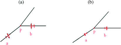
(a) Scenario of convergence of flight (b) scenario of crossing after passing
-
(2)
Two aircraft A and B crossing after passing intersection P (Fig. 3(b)). Still consider worst circumstance, aircraft B has reached to P, aircraft A still maintain original flight state. So the aircraft A is still in the area where the protection areas are overlapped, conflict still exists.

So, the neighborhood of P is defined as the scope of assessment of controller intervention degree.
Where x p , y p , z p is the coordinate and altitude of intersection P.
4.1 Assessment of Controller Intervention Degree
The change of flight elements indicates the happen of controller intervention, then define P c as intervention degree:
Where, n is the number of trajectory points in certain scope of intersection, p i is the i-th trajectory points.
The statistical methods for the change of flight elements are described below.
4.2 Statistical Probability for the Change of Flight Elements
Constructing Cartesian Coordinate System in Spatial Range of airspace, take neighborhood ɛ (Eq. (4)) as the conflicts statistics scope of an intersection, we call it as overlap area.
As the civil aircraft has certain stability, flight elements do not change immediately after maneuvering instruction. And in actual flight, the aircraft is often affected by the air flow which will cause slight disturbance. So in order to accurately detect the change of flight elements, the status change time should be analyzed.
According to the maneuvering delay time from ICAO PANs-OPS, in arrival flight segment, pilot reaction delay is 0–6 s, operating delay is 0–5 s. In departure segment, pilot reaction delay is 0–3 s, operating delay is 0–3 s. the data is relatively conservative, and autopilot is the main method in actual flight. So, 4 s flight reaction delay and 5 s maneuvering delay are adopted in this paper as the basis for detect the changes of flight elements.
4.2.1 Detection of Altitude Change
Points appearing in the overlap area are extracted by the flight number and stored separately. Each point sequenced according to time. Take t = 3 as change judgment step size. Assume t1 is the earliest time enter into the overlap area, t2 is the latest time enter into the overlap area. Assume A(t′) is the point altitude at time t′.
Check each flight points from t1 to t2:
-
(1)
when \( {\text{A}}(t_{1} ) \ne {\text{A}}(t_{1} + nt) \cdot \left( {n = 1, 2, 3\ldots \ldots } \right),{\text{ let }}t_{1}^{'} = t_{1} + nt \), keep checking, until \( {\text{A}}(t_{1}^{'} + nt) = {\text{A}}[t_{1}^{'} + \left( {n + 1} \right)t],{\text{ then let}}t_{2}^{'} = t_{1}^{'} + nt \), or
-
(2)
when \( {\text{A}}(t_{1} ) = {\text{A}}(t_{1} + nt) \, .\left( {n = 1, 2, 3\ldots \ldots } \right),{\text{ let }}t_{1}^{'} = t_{1} + nt \), keep checking, until \( {\text{A}}(t_{1}^{'} + nt) \ne {\text{A}}[t_{1}^{'} + \left( {n + 1} \right)t],\quad {\text{then let }}t_{2} = t_{1}^{'} + nt \).
If \( t_{2}^{'} - t_{1}^{'} \le \, 6 {\text{s}} \), the altitude change is neglected; if \( t_{2}^{'} - t_{1}^{'} \le \, 6 {\text{s}} \), calculate the inequality (6).
If the inequality is true, altitude change happened in specific time period, and \( f_{A} (p_{i} ) = 1\,{\text{f}}_{\text{A}} \left( {{\text{p}}_{\text{i}} } \right) \) otherwise \( f_{A} (p_{i} ) = 0 \).
4.2.2 Detection of Heading Change
Assume point i(x i ,y i ) is the earliest point where certain flight enter into the overlap area, point j(x j ,y j ) is the location of point of the flight. Great circle of track angle (α) is calculated:
Check each flight points from \( t1\,{\text{to}}\,t2 \). When \( \alpha (t_{1} ) \ne \alpha (t_{1} + nt).\left( {{\text{n}} = 1, 2, 3\ldots \ldots } \right) \)时, \( {\text{let }}t_{1}^{'} = t_{1} + nt \). keep checking, until \( \alpha (t_{1}^{'} + nt) = \alpha [t_{1}^{'} + \left( {n + 1} \right)t)] \), then let \( t_{2}^{'} = t_{1}^{'} + nt \). If \( t_{2}^{'} - t_{1}^{'} \le 6\text{s} \), the change is neglected; if \( t_{2}^{'} - t_{1}^{'} > 6\text{s} \), calculate the inequality (8).
If the inequality is true, heading change happened in specific time period, and \( f_{H} (p_{i} ) = 1\,{\text{f}}_{\text{A}} \left( {{\text{p}}_{\text{i}} } \right) \) otherwise \( f_{H} (p_{i} ) = 0 \).
4.2.3 Detection of Speed Change
In actual flight, flight speed is generally adjusted for every 10 knots, however, considering the change of airflow, speed of change may not be an integer multiple of 10. Troposphere is the main area for operation of aircraft, and the average speed of wind is 12.2 m/s ≈ 2knot, so we consider 8 knots as the change of speed.
Assume \( C\left( {t^{'} } \right) \) is the speed of point at time \( {\text{t}}^{'} \). Check each flight points from \( t1\,{\text{to}}\,t2 \), when speed of aircraft \( C(t_{1} ) \ne {\text{C}}(t_{1} + {\text{nt}})\, \left( {n = 1, 2, 3\ldots \ldots } \right) \), let \( t_{1}^{'} = t_{1} + nt \). Keep checking untile \( C(t_{1}^{'} + {\text{nt}}) = C[t_{1}^{'} + \left( {n + 1} \right)t)] \), then let \( t_{2}^{'} = t_{2}^{'} + nt \). Calculate the inequality (9).
If the inequality is true, speed change happened in specific time period, and \( f_{v} (p_{i} ) = 1\,{\text{f}}_{\text{A}} \left( {{\text{p}}_{\text{i}} } \right) \), otherwise \( f_{v} (p_{i} ) = 0 \).
5 Experimental Evaluation
In order to verify the evaluation method, 24 h ADS-B surveillance data of Tianjin airport is used to assess the controller intervention degree. Data collection step is 3 min, coordinates of trajectory points is correspond to the WGS-84 system.
5.1 Generation of Density Distribution Array
Sub-cluster of each trajectory point should be generated, before that the radius r of density distribution is determined. The size of the radius r affects the speed and the result of clustering. In some literatures, the k neighborhood algorithm is used to generate the distance d i from the k-nearest neighborhood for each points, the r is the average of all d i . However, large amount of data is used for analysis, and whether or not r is appropriate depends on the value of k. so as to improve it, r is determined according to speed limitation and data collection frequency in this paper. Assume the speed limitation is \( V_{\hbox{max} } \), t is the step size of data collection, r is determined as: \( r = V_{\hbox{max} } \times t \).
If t is too small, it is difficult to identify the isolated point. On the contrary, if t is too large, it is unfavorable for further clustering. In this case, we use t = 5s to generate sub-cluster for each point. Trajectory points are sorted by dps i of sub-cluster for each point. In Tianjin airport, maximum IAS is 210kt, so we use r = 540 m to generate sub-cluster. The optimal two-division method described in 2.2 is used to category each point. The relationship between number of segments and total variance is showed in Fig. 4.

Relationship between number of partition and variance
In Fig. 4, we can clearly see that the inflection point of total variance corresponds to number of segments is 11. Tag each point according to division result. In this experiment, number of elements contained in sub-cluster of each point evenly distributed from 0 to 1089. Because the existence of error happens in ADS-B data collection and analysis, noisy data should be deleted to prevent the effect to the outcome. So, points with small number (0–10) contained in sub-cluster is deleted as noise. The final segment number is 7, the density tag is 1–7, 7 means highest density.
5.2 Intersection Determination
Maximum IAS is 210kt, lv = 390, bank angle α = 15 is used to generate the average trajectory. The average trajectory is showed in Fig. 5. Where, blue represents departure, red represents arrival. P1, P2, P3 and P4 are determined intersections.

Average trajectory and intersection distribution (Color figure online)
5.3 Result of Controller Intervention Assessment
The controller intervention assessment result is illustrated in Table 1.
It can be seen from Fig. 5, P2 and P3 is closer than with other intersections, and the distance along same track is less than lateral minima. So, to aircraft with same flight path, enter into the overlap area of P2 also effect the aircraft around P3. However, it is impossible to know from historical data whether p2 or p3 is it’s conflict point. And the time when it enter into the overlap area of is also unknown. In this paper, we consider a point between two intersections as the equivalent intersection, so that the intervention degree of the new intersection P23 is approximately equal to the average intervention degree of P2 and P3. Overlap area of P23 will be equivalent to the overlap area of P2 and P3 for aircraft with P2 or P3 as the direct collision point. This can be as a control reference in actual work of controller. The location of P23 can be located: because P2 and P3 are on the same path, so according to the intervention degree of P2 and P3, the location of P23 is on the proportional position of intervention degree of P2 and P3.
5.4 Result Analysis
In experimental airports, due to airspace restrictions, nearly 70% traffic concentrate in the west of airport, and much intervention is needed to solve the conflict, so the intervention degree is larger. The result (Table 1) shows consistency with actual operation. P2 and P3 are conflict points of departure and arrival, intervention degree of P3 is larger because from P3 the departure path divided into two branches, and both of them have potential conflict with arrival flight on the following flight (P1 and P2). And this is the reason for smaller intervention degree of P1 and P2. P4 is close to runway, the altitude of departure aircraft is low, and the arrival aircraft is high, vertical separation is guaranteed automatically, so the intervention degree is small.
As the analysis above, P3 cause large workload for controller, this can be as a reference to airspace redesign.
6 Conclusion
In this paper, we have proposed a method to evaluate the controller intervention degree through analysing the historic surveillance data. Because the amount of data used is large, so improved density based clustering algorithm is adopted to generate the average flight trajectory. Here, trajectory clustering is divided into two steps. Because the density of flight data is uneven, the efficiency and accuracy of clustering will be effected seriously. So, sub-clusters are generated first to understand the overall density distribution of data sample, and sub-clusters are divided into several categories according to density. Optimal two- partition method is used to determine the number of categories. Sub-clusters with similar density is marked with same density tag and put into same category. Then, SNN algorithm is used to cluster sub-clusters with same density tag to generate average trajectory. The intersection of trajectory is the potential conflicts point which is used for controller intervention degree calculation. Controller intervention degree is defined as statistical probability of change of flight elements. So, for the purpose of statistic, the scope of intervention area is analysed and the detection method of flight elements changes is proposed. Finally, surveillance data of an airport is used to verify the method. The experimental results show that this method can obtain the distribution of conflict and controller pressure points in the terminal area, and the result is quite consistent with reality. The controller intervention degree can be used as a reference for further airspace designation.
References
Meyn, L.A., Erzberger, H.: Estimating controller intervention probabilities for optimized profile descent arrivals. In: 11th AIAA Aviation Technology, Integration, and Operations (ATIO) Conference, 20–22 September 2011. AIAA 2011-6802
Gariel, M., Srivastava, A., Feron, E.: Trajectory clustering and an application to airspace monitoring. Intell. Transp. Syst. 12(4), 1511–1524 (2011)
Wang, C., Xu, X., Wang, F.: ATC serviceability analysis of terminal arrival procedures using trajectory clusting. J. Nanjing Univ. Aeronaut. Astronaut. 45(1), 130–139 (2013)
ICAO: Procedure for air navigation services—aircraft operation construction of visual and instrument flight procedures. Doc8168-OPS/611, vol. II (2006)
Bilimoria, K.D., Lee, H.Q., Oaks, R.: Properties of air traffic conflicts for free and structured routing. In: Proceedings of the American Institute of Aeronautics and Astronautics (AIAA) Guidance, Navigation, and Control Conference, 6–9 August 2001
Proceedings of the AIAA Modeling, Simulation and Technology Conference, Keystone, Colorado, 21–24 August 2006 (EIWAC), Tokyo, Japan, March 2009
Wang, C., Han, B.C., Wang, F.: Track traffic flow identification method based on track spectrum clustering in terminal area. J. Southwest Jiaotong Univ. 49(3), 546–552 (2014)
Author information
Authors and Affiliations
Corresponding author
Editor information
Editors and Affiliations
Rights and permissions
Copyright information
© 2017 Springer International Publishing AG
About this paper
Cite this paper
Qi, Y., Wang, X., Zhang, X. (2017). Controller Intervention Degree Evaluation of Intersection in Terminal Airspace. In: Harris, D. (eds) Engineering Psychology and Cognitive Ergonomics: Performance, Emotion and Situation Awareness. EPCE 2017. Lecture Notes in Computer Science(), vol 10275. Springer, Cham. https://doi.org/10.1007/978-3-319-58472-0_29
Download citation
DOI: https://doi.org/10.1007/978-3-319-58472-0_29
Published:
Publisher Name: Springer, Cham
Print ISBN: 978-3-319-58471-3
Online ISBN: 978-3-319-58472-0
eBook Packages: Computer ScienceComputer Science (R0)