Separating Semantic and Circular Security for Symmetric-Key Bit Encryption from the Learning with Errors Assumption

Abstract

In this work we separate private-key semantic security from 1-circular security for bit encryption using the Learning with Error assumption. Prior works used the less standard assumptions of multilinear maps or indistinguishability obfuscation. To achieve our results we develop new techniques for obliviously evaluating branching programs.

B. Waters—Supported by NSF CNS-1228599 and CNS-1414082, DARPA SafeWare, Microsoft Faculty Fellowship, and Packard Foundation Fellowship.

1 Introduction

Over the past several years the cryptographic community has given considerable attention to the notion of key-dependent message security. In key dependent security we consider an attacker that gains access to ciphertexts that encrypt certain functions of the secret key(s) of the user(s). Ideally, a system should remain semantically secure even in the presence of this additional information.

One of the most prominent problems in key dependent message security is the case of circular security. A circular secure system considers security in the presence of key cycles. A key cycle of k users consists of k encryptions where the i-th ciphertext $\mathsf {ct}_i$ is an encryption of the i+1 user’s secret key under user i’s public key. That is $\mathsf {ct}_1 = \mathsf {Encrypt}(\mathrm {PK}_1,\mathrm {SK}_2), \mathsf {ct}_2 = \mathsf {Encrypt}(\mathrm {PK}_2,\mathrm {SK}_3) \ldots , \mathsf {ct}_k = \mathsf {Encrypt}(\mathrm {PK}_k,\mathrm {SK}_1)$. If a system is k circular secure, then such a cycle should be indistinguishable from an encryption of k arbitrary messages. The notion also applies to secret key encryption systems.

One reason that circular security has received significant attention is that the problem has arisen in multiple applications [2, 16, 27], the most notable is that Gentry [22] showed how a circular secure leveled homomorphic encryption can be bootstrapped to homomorphic encryption that works for circuits of unbounded depth. Stemming from this motivation there have been several positive results [4,5,6, 8, 11, 13, 14, 29] that have achieved circular and more general notations of key dependent messages security from a variety of cryptographic assumptions.

On the flip side several works have sought to discover if there exist separations between IND-CPA security and different forms of circular security. That is they sought to develop a system that was not circular secure, but remained IND-CPA secure. For the case of 1-circular security achieving such a separation is trivial. The (secret key) encryption system simply tests if the message to be encrypted is equal to the secret key $\mathrm {SK}$, if so it gives the message in the clear; otherwise it encrypts as normal. (This example can be easily extended to public key encryption.) Clearly, such a system is not circular secure and it is easy to show it maintains IND-CPA security. More work is required, however, to achieve separations of length greater than one. Separations were first shown for the case of $k=2$ length cycles using groups with bilinear maps [1, 17] and later [10] under the Learning with Errors assumption [34]. Subsequently, there existed works that achieved separations for arbitrary length cycles [25, 28], however, these required the use obfuscation. All current candidates of general obfuscation schemes rely on the relatively new primitive of multilinear maps, where many such multilinear map candidates have suffered from cryptanalysis attacks [18, 19]. Most recently and Alamati and Peikert [3] and Koppula and Waters [26] showed separations of arbitrary length cycles from the much more standard Learning with Errors assumption.

Another challenging direction in achieving separations for circular security is to consider encryptions systems where the message consist of a single bit. Separating from IND-CPA is difficult even in the case of cycles of length 1 (i.e. someone encrypts their own secret key). Consider a bit encryption system with keys of length $\ell =\ell (\lambda )$. Suppose an attacker receives an encryption of the secret key in the form of $\ell$ successive bit by bit encryptions. Can this be detected?

We observe that encrypting bit by bit seems to make detection harder. Our trivial counterexample from above no longer applies since the single bit message cannot be compared to the much longer key. The first work to consider such a separation was due to Rothblum [35] who showed that a separation could be achieved from multilinear maps under certain assumptions. One important caveat, however, to his result was that the level of multilinearlity must be greater than $\log (q)$ where q is the group order. This restriction appears to be at odds with current multilinear map/encoding candidates which are based off of “noisy cryptography” and naturally require a bigger modulus whose log is greater than the number of multiplications allowed. Later, Koppula, Ramchen and Waters [25] showed how to achieve a separation from bit encryption using indistinguishability obfuscation. Again, such a tool is not known from standard assumptions.

In this work we aim to separate semantic security from 1-circular security for bit encryption systems under the Learning with Errors assumption. Our motivation to study this problem is two fold. First, achieving such a separation under a standard assumption will significantly increase our confidence compared to obfuscation or multilinear map-based results. Second, studying such a problem presents the opportunity for developing new techniques in the general area of computing on encrypted data and may lead to other results down the line.

To begin with, we wish to highlight some challenges presented by bit encryption systems that were not addressed in prior work. First, the recent results of [3, 26] both use a form of telescoping cancellation where the encryption algorithm takes in a message and uses this as a ‘lattice trapdoor’ [24, 30]; if the message contained the needed secret key then it cancels out the public key of an “adjacent” ciphertext. We observe that such techniques require an encryption algorithm that receives the entire secret key at once, and there is no clear path to leverage this in the case where an encryption algorithm receives just a single bit message. Second, while the level restriction in Rothblum’s result [35] appeared in the context of multilinear maps, the fundamental issue will transcend to our Learning with Errors solution. Looking ahead we will need to perform a computation where the number of multiplication steps is restricted to be less than $\log (q)$, where here q is the modulus we work in.

1.1 Separations from Learning with Errors

We will now describe our bit encryption scheme that is semantically secure but not circular secure. Like previous works [3, 10, 26], we will take decryption out of the picture, and focus on building an ${\mathsf{IND}}{\text {-}}{\mathsf{CPA}}$ secure encryption scheme where one can distinguish between an encryption of the secret key and encryptions of zeroes.

The two primary ingredients of our construction are low-depth pseudorandom functions (PRFs) and lattice trapdoors. In particular, we require a PRF which can be represented using a permutation branching program of polynomial length and polynomial width.¹ Banerjee, Peikert and Rosen [7] showed how to construct LWE based PRFs that can be represented using $\mathbf {NC}^1$ circuits, and using Barrington’s theorem [9], we get PRFs that can be represented using branching programs of polynomial length and width 5.

Next, let us recall the notion of lattice trapdoors. A lattice trapdoor generation algorithm outputs a matrix $\mathbf {A}$ together with a trapdoor $T_{\mathbf {A}}$. The matrix looks uniformly random, while the trapdoor can be used to compute, for any matrix $\mathbf {U}$, a low norm matrix $\mathbf {S} = \mathbf {A}^{-1}(\mathbf {U})$ such that $\mathbf {A}\cdot \mathbf {S} = \mathbf {U}$.² As a result, the matrix $\varvec{\mathrm {S}}$ can be used to ‘transform’ the matrix $\varvec{\mathrm {A}}$ to another matrix $\varvec{\mathrm {U}}$. In this work, we will be interested in oblivious sequence transformation: we want a sequence of matrices $\varvec{\mathrm {B}}_1, \ldots , \varvec{\mathrm {B}}_w$ such that for any sequence of matrices $\varvec{\mathrm {U}}_1, \ldots , \varvec{\mathrm {U}}_w$, we can compute a low norm matrix $\varvec{\mathrm {S}}$ such that $\varvec{\mathrm {B}}_i\cdot \varvec{\mathrm {S}} = \varvec{\mathrm {U}}_i$. Note that the same matrix $\varvec{\mathrm {S}}$ should be able to transform any $\varvec{\mathrm {B}}_i$ to $\varvec{\mathrm {U}}_i$; that is, $\varvec{\mathrm {S}}$ is oblivious of i. This obliviousness property will be important for our solution, and together with the telescoping products/cascading cancellations idea of [3, 23, 26], we get our counterexample.

Oblivious Sequence Transformation. We first observe that one can easily obtain oblivious sequence transformation, given standard lattice trapdoors. Consider the following matrix $\varvec{\mathrm {B}}$:

$$ \varvec{\mathrm {B}} = \begin{bmatrix} \varvec{\mathrm {B}}_1 \\ \vdots \\ \varvec{\mathrm {B}}_w\\ \end{bmatrix}. $$

Let T denote the trapdoor of $\varvec{\mathrm {B}}$ (we will refer to T as the ‘joint trapdoor’ of $\varvec{\mathrm {B}}_1$, $\ldots$, $\varvec{\mathrm {B}}_w$). Now, given any sequence $\varvec{\mathrm {U}}_1, \ldots , \varvec{\mathrm {U}}_w$, we similarly define a new matrix $\varvec{\mathrm {U}}$ which has the $\varvec{\mathrm {U}}_i$ stacked together, and set $\varvec{\mathrm {S}} = \varvec{\mathrm {B}}^{-1}(\varvec{\mathrm {U}})$. Clearly, this satisfies our oblivious sequence transformation requirement.

Our Encryption Scheme. As mentioned before, we will only focus on the setup, encryption and testing algorithms. Let $\mathrm {PRF}$ be a pseudorandom function family with keys and inputs of length $\lambda$, and output being a single bit. For any input i, we require that the function $\mathrm {PRF}(\cdot , i)$ can be represented using a branching program of length L and width 5 (we choose 5 for simplicity here; our formal description works for any polynomial width w). The setup algorithm chooses a PRF key s. Let $\mathsf {nbp}$ be a parameter which represents the number of points at which the PRF is evaluated, and let $t_i = \mathrm {PRF}(s, i)$ for $i\le \mathsf {nbp}$. Finally, for each $i\le \mathsf {nbp}$, let $\mathsf {BP}^{(i)}$ denote the branching program that evaluates $\mathrm {PRF}(\cdot , i)$. Each branching program $\mathsf {BP}^{(i)}$ has L levels and 5 possible states at each level. At the last level, there are only two valid states — $\mathsf {acc}^{(i)}$ and $\mathsf {rej}^{(i)}$, i.e. the accepting and rejecting state. For each branching program $\mathsf {BP}^{(i)}$ and level j, there are two state transition functions $\sigma ^{(i)}_{j, 0}, \sigma ^{(i)}_{j, 1}$ that decide the transition between states depending upon the input bit read. The setup algorithm also chooses, for each branching program $\mathsf {BP}^{(i)}$, level $j\le L$ and state $k \le 5$, a matrix $\varvec{\mathrm {B}}^{(i)}_{j, k}$. At all levels $j \ne L$, the matrices $\varvec{\mathrm {B}}^{(i)}_{j, 1}, \ldots , \varvec{\mathrm {B}}^{(i)}_{j, 5}$ have a joint trapdoor. At the top level, the matrices satisfy the following relation:

$$ \sum _{i\ :\ t_i = 0} \varvec{\mathrm {B}}^{(i)}_{L, \mathsf {rej}^{(i)}} + \sum _{i\ :\ t_i = 1} \varvec{\mathrm {B}}^{(i)}_{L, \mathsf {acc}^{(i)}} = \varvec{\mathrm {0}}. $$

The secret key consists of the PRF key s and $\mathsf {nbp}\cdot L$ trapdoors $T^{(i)}_j$.

The encryption algorithm is designed specifically to distinguish key encryptions from encryptions of zeros. Each ciphertext consists of L sub-ciphertexts, one for each level, and each sub-ciphertext consists of $\mathsf {nbp}$ sub-sub-ciphertexts. The sub-sub-ciphertext corresponding to $\mathsf {BP}^{(i)}$ at level j can be used to transform $\varvec{\mathrm {B}}^{(i)}_{j, k}$ to $\varvec{\mathrm {B}}^{(i)}_{j + 1, \sigma ^{(i)}_{j, 0}(k)}$ or $\varvec{\mathrm {B}}^{(i)}_{j + 1, \sigma ^{(i)}_{j, 1}(k)}$, depending on the bit encrypted. This is achieved via oblivious sequence transformation. Let b denote the bit encrypted, and let $\varvec{\mathrm {D}}$ be the matrix constructed by stacking $\{\varvec{\mathrm {B}}^{(i)}_{j, 1}, \ldots , \varvec{\mathrm {B}}^{(i)}_{j, 5}\}$ according to the permutation $\sigma ^{(i)}_{j, b}$. The sub-sub-ciphertext $\mathsf {ct}^{(i)}_j$ for program $\mathsf {BP}^{(i)}$ at level j is simply (a noisy approximation of) ${\varvec{\mathrm {B}}^{(i)}_j}^{-1}(\varvec{\mathrm {D}})$. The ciphertext also includes the base matrices $\{\varvec{\mathrm {B}}^{(i)}_0\}$ for each program.

The testing algorithm is used to distinguish between an encryption of the secret key and encryptions of zeros. It uses the first $|s| = \lambda$ ciphertexts, which are either encryptions of the PRF key s, or encryptions of zeros. Let us consider the case where the $\lambda$ ciphertexts are encryptions of s. At a high level, the testing algorithm combines the ciphertext components appropriately, such that for each $i\le \mathsf {nbp}$, the result is $\varvec{\mathrm {B}}^{(i)}_{L, \mathsf {rej}^{(i)}}$ if $\mathrm {PRF}(s, i) = 0$, and $\varvec{\mathrm {B}}^{(i)}_{L, \mathsf {acc}^{(i)}}$ otherwise. Once the testing algorithm gets these matrices, it can sum them to check if it is (close to) the zero matrix. The testing algorithm essentially mimics the program evaluation on s using the encryption of s. Let us fix a program $\mathsf {BP}^{(i)}$, and say it reads bit positions $p_1, \ldots , p_L$. At step 1, the program goes from state 1 at level 0 to state $\mathsf {st}_1 = \sigma ^{(i)}_{1, s_{p_1}}$ at level 1. The test algorithm has $\varvec{\mathrm {B}}^{(i)}_{0,1}$. It combines this with the (i, 1) component of the $p_1^{th}$ ciphertext to get $\varvec{\mathrm {B}}^{(i)}_{1,\mathsf {st}_1}$. Next, the program reads the bit at position $p_2$ and goes to state $\mathsf {st}_2$ at level 2. The test algorithm, accordingly, combines $\varvec{\mathrm {B}}^{(i)}_{1,\mathsf {st}_1}$ with the (i, 2) sub-sub-component of the $p_2^{th}$ ciphertext to compute $\varvec{\mathrm {B}}^{(i)}_{2,p_2}$. Proceeding this way, the actual program evaluation reaches either $\mathsf {acc}^{(i)}$ or $\mathsf {rej}^{(i)}$, and the test algorithm accordingly reaches either $\varvec{\mathrm {B}}^{(i)}_{L,\mathsf {acc}^{(i)}}$ or $\varvec{\mathrm {B}}^{(i)}_{L, \mathsf {rej}^{(i)}}$.

The solution described above, however, is not ${\mathsf{IND}}{\text {-}}{\mathsf{CPA}}$ secure. To hide the encrypted bit without affecting the above computation, we will have to add some noise to each sub-sub-ciphertext. In particular, instead of outputting ${\varvec{\mathrm {B}}^{(i)}_j}^{-1}(\varvec{\mathrm {D}})$ for some matrix $\varvec{\mathrm {D}}$, we will now have ${\varvec{\mathrm {B}}^{(i)}_j}^{-1}(\varvec{\mathrm {S}}\cdot \varvec{\mathrm {D}} + \mathsf {noise})$,³ where $\varvec{\mathrm {S}}$ is a low norm matrix. To prove ${\mathsf{IND}}{\text {-}}{\mathsf{CPA}}$ security, we first switch the top level matrices to uniformly random matrices. Once we’ve done that, we can use $\mathsf {LWE}$, together with the properties of lattice trapdoors, to argue that the top level sub-sub-ciphertexts look like random matrices from a low-norm distribution. As a result, we don’t need trapdoors for the matrices at level $L-1$, and hence, they can be switched to uniformly random matrices. Using $\mathsf {LWE}$ with trapdoor properties, we can then switch the sub-sub-ciphertexts at level $L-1$ to random matrices. Proceeding this way, all sub-sub-ciphertexts can be made random Gaussian matrices. This concludes our proof.

Separation from Chosen Ciphertext Security. One interesting question is whether achieving chosen ciphertext security (as opposed to IND-CPA security) makes a bit encryption system more likely to be resistant to circular security attacks. Here we show generically that achieving a bit encryption system that is IND-CCA secure, but not circular secure is no more difficult than our original separation problem. In particular, we show generically how to combine a IND-CPA secure, but not circular secure bit encryption with multi-bit CCA secure encryption to achieve a single bit encryption system that is IND-CPA secure. We note that Rothblum addressed CCA security, but used the more specific assumption of trapdoor permutations to achieve NIZKs.

Our transformation is fairly simple and follows in a similar manner to how an analogous theorem in Bishop, Hohenberger and Waters [10].

Relation to GGH15 Graph Based Multilinear Maps. Our counterexample construction bears some similarities to the graph-induced multilinear maps scheme of Gentry, Gorbunov and Halevi [23]. In a graph induced multilinear maps scheme, we have an underlying graph G, and encodings of elements are relative to pairs of connected nodes in in the graphs. Given encodings of $s_1$ and $s_2$ relative to connected nodes $u \rightsquigarrow v$, one can compute an encoding of $s_1 + s_2$ relative to $u \rightsquigarrow v$. Similarly, given an encoding of $s_1$ relative to $u \rightsquigarrow v$ and an encoding of $s_2$ relative to $v \rightsquigarrow w$, one can compute an encoding of $s_1 \cdot s_2$ relative to $u \rightsquigarrow w$. Finally, one is allowed to zero-test corresponding to certain source-destination pairs. Gentry et al. gave a lattice based construction for graph-induced encoding scheme, where each vertex u has an associated matrix ${\mathbf {A}_{{\varvec{u}}}}$ (together with a trapdoor $T_u$). The encoding of an element s corresponding to the edge (u, v) is simply ${\mathbf {A}_{{\varvec{u}}}^{-1}}(s \mathbf {A}_{{\varvec{v}}} + \mathsf {noise})$.

At a high level, our construction looks similar to the GGH15 multilinear maps construction. In particular, while GGH15 uses the cascading cancellations property to prove correctness, we use it for proving that the testing algorithm succeeds with high probability. Our security requirements, on the other hand, are different from that in multilinear maps. However, we believe that the ideas used in this work can be used to prove security of GGH15 mmaps for special graphs/secret distributions (note that GGH15 gave a candidate multilinear maps construction, and it did not have a proof of security for general graphs).

Summary and Conclusions. To summarise, we show how to perform computation using an outside primitive by means of our oblivious sequence transformation approach. This allows us to show a separation between private-key semantic security and circular security for bit encryption schemes. While such counterexamples are contrived and do not give much insight into the circular security of existing schemes, we see this as a primitive of its own. The tools/techniques used for developing such counterexamples might have other applications. In particular, these counterexamples share certain features with more advanced cryptographic primitives such as witness encryption and code obfuscation.

2 Preliminaries

Notations. We will use lowercase bold letters for vectors (e.g. $\varvec{\mathrm {v}}$) and uppercase bold letters for matrices (e.g. $\mathbf {A}$). For any finite set S, $x\leftarrow S$ denotes a uniformly random element x from the set S. Similarly, for any distribution $\mathcal {D}$, $x \leftarrow \mathcal {D}$ denotes an element x drawn from distribution $\mathcal {D}$. The distribution $\mathcal {D}^n$ is used to represent a distribution over vectors of n components, where each component is drawn independently from the distribution $\mathcal {D}$.

Min-Entropy and Randomness Extraction. The min-entropy of a random variable X is defined as . Let $\mathsf {SD}(X, Y)$ denote the statistical distance between two random variables X and Y. Below we state the Leftover Hash Lemma (LHL) from [20, 21].

Theorem 1

Let $\mathcal {H}= \left\{ h\ :\ X \rightarrow Y \right\} _{h \in \mathcal {H}}$ be a universal hash family, then for any random variable W taking values in X, the following holds

$$ \mathsf {SD}\left( \left( h, h(W) \right) , \left( h, U_Y \right) \right) \le \dfrac{1}{2} \sqrt{2^{- \varvec{\mathrm {H}}_\infty \left( W \right) } \cdot |Y|}. $$

We will use the following corollary, which follows from the Leftover Hash Lemma.

Corollary 1

Let $\ell > m \cdot n \log _2 q + \omega (\log n)$ and q a prime. Let $\varvec{\mathrm {R}}$ be an $k \times m$ matrix chosen as per distribution $\mathcal {R}$, where $k = k(n)$ is polynomial in n and $\varvec{\mathrm {H}}_\infty \left( \mathcal {R} \right) = \ell$. Let $\varvec{\mathrm {A}}$ and $\varvec{\mathrm {B}}$ be matrices chosen uniformly in $\mathbb {Z}_q^{n \times k}$ and $\mathbb {Z}_q^{n \times m}$, respectively. Then the statistical distance between the following distributions is negligible in n.

$$ \left\{ \left( \varvec{\mathrm {A}}, \varvec{\mathrm {A}} \cdot \varvec{\mathrm {R}} \right) \right\} \approx _s \left\{ \left( \varvec{\mathrm {A}}, \varvec{\mathrm {B}} \right) \right\} $$

Proof

The proof of above corollary follows directly from the Leftover Hash Lemma. Note that for a prime q the family of hash functions $h_{\varvec{\mathrm {A}}} : \mathbb {Z}_q^{k \times m} \rightarrow \mathbb {Z}_q^{n \times m}$ for $\varvec{\mathrm {A}} \in \mathbb {Z}_q^{n \times k}$ defined by $h_{\varvec{\mathrm {A}}}(\varvec{\mathrm {X}}) = \varvec{\mathrm {A}} \cdot \varvec{\mathrm {X}}$ is universal. Therefore, if $\mathcal {R}$ has sufficient min-entropy, i.e. $\ell > m \cdot n \log _2 q + \omega (\log n)$, then the Leftover Hash Lemma states that statistical distance between the distributions $\left( \varvec{\mathrm {A}}, \varvec{\mathrm {A}} \cdot \varvec{\mathrm {R}} \right)$ and $\left( \varvec{\mathrm {A}}, \varvec{\mathrm {B}} \right)$ is at most $2^{- \omega (\log n)}$ which is negligible in n as desired.

2.1 Lattice Preliminaries

This section closely follows [26].

Given positive integers n, m, q and a matrix $\varvec{\mathrm {A}} \in \mathbb {Z}_q^{n \times m}$, we let $\varLambda _q^\perp (\varvec{\mathrm {A}})$ denote the lattice $\{\varvec{\mathrm {x}} \in \mathbb {Z}^m \; : \; \varvec{\mathrm {A}} \cdot \varvec{\mathrm {x}} = \varvec{\mathrm {0}} \mod q\}$. For $\varvec{\mathrm {u}} \in \mathbb {Z}_q^n$, we let $\varLambda _q^{\varvec{\mathrm {u}}}(\varvec{\mathrm {A}})$ denote the coset $\{\varvec{\mathrm {x}} \in \mathbb {Z}^m \; : \; \varvec{\mathrm {A}} \cdot \varvec{\mathrm {x}} = \varvec{\mathrm {u}} \mod q\}$.

Discrete Gaussians. Let $\sigma$ be any positive real number. The Gaussian distribution $\mathcal {D}_{\sigma }$ with parameter $\sigma$ is defined by the probability distribution function $\rho _{\sigma }(\varvec{\mathrm {x}}) = \exp (-\pi \cdot ||\varvec{\mathrm {x}} ||^2/\sigma ^2)$. For any set $\mathcal {L}\subset \mathcal {R}^m$, define $\rho _{\sigma }(\mathcal {L}) = \sum _{\varvec{\mathrm {x}} \in \mathcal {L}} \rho _{\sigma }(\varvec{\mathrm {x}})$. The discrete Gaussian distribution $\mathcal {D}_{\mathcal {L}, \sigma }$ over $\mathcal {L}$ with parameter $\sigma$ is defined by the probability distribution function $\rho _{\mathcal {L}, \sigma }(\varvec{\mathrm {x}}) = \rho _{\sigma }(\varvec{\mathrm {x}})/\rho _{\sigma }(\mathcal {L})$ for all $\varvec{\mathrm {x}} \in \mathcal {L}$.

The following lemma (Lemma 4.4 of [24, 31]) shows that if the parameter $\sigma$ of a discrete Gaussian distribution is small, then any vector drawn from this distribution will be short (with high probability).

Lemma 1

Let m, n, q be positive integers with $m > n$, $q\ge 2$. Let $\mathbf {A} \in \mathbb {Z}_q^{n\times m}$ be a matrix of dimensions $n\times m$, $\sigma = \tilde{\varOmega }(n)$ and $\mathcal {L}= \varLambda _{q}^{\perp }(\mathbf {A})$. Then

$$ \Pr [|| \varvec{\mathrm {x}} || > \sqrt{m} \cdot \sigma : \varvec{\mathrm {x}} \leftarrow \mathcal {D}_{\mathcal {L}, \sigma } ] \le negl(n). $$

Learning with Errors (LWE). The Learning with Errors (LWE) problem was introduced by Regev [34]. The LWE problem has four parameters: the dimension of the lattice n, the number of samples m, the modulus q and the error distribution $\chi (n)$.

Assumption 1

(Learning with Errors). Let n, m and q be positive integers and $\chi$ a noise distribution on $\mathbb {Z}$. The Learning with Errors assumption $(n, m, q, \chi ){\text {-}}\mathsf {LWE}$, parameterized by $n, m, q, \chi$, states that the following distributions are computationally indistinguishable:

$$ \left\{ (\mathbf {A}, \varvec{\mathrm {s}}^{\top } \cdot \mathbf {A} + \varvec{\mathrm {e}}) \; : \; \begin{array}{l} \mathbf {A} \leftarrow \mathbb {Z}_q^{n\times m},\\ \varvec{\mathrm {s}} \leftarrow \mathbb {Z}_q^{n}, \varvec{\mathrm {e}} \leftarrow \chi ^{m} \end{array} \right\} \approx _c \left\{ (\mathbf {A}, \varvec{\mathrm {u}}) \; : \; \begin{array}{l} \mathbf {A} \leftarrow \mathbb {Z}_q^{n \times m},\\ \varvec{\mathrm {u}} \leftarrow \mathbb {Z}_q^{m} \end{array} \right\} $$

Under a quantum reduction, Regev [34] showed that for certain noise distributions, LWE is as hard as worst case lattice problems such as the decisional approximate shortest vector problem ($\mathsf {GapSVP}$) and approximate shortest independent vectors problem ($\mathsf {SIVP}$). The following theorem statement is from Peikert’s survey [33].

Theorem 2

([34]). For any $m\le \mathsf {poly}(n)$, any $q \le 2^{\mathsf {poly}(n)}$, and any discretized Gaussian error distribution $\chi$ of parameter $\alpha \cdot q \ge 2\cdot \sqrt{n}$, solving $(n, m, q, \chi ) {\text {-}}\mathsf {LWE}$ is as hard as quantumly solving $\mathsf {GapSVP}_{\gamma }$ and $\mathsf {SIVP}_{\gamma }$ on arbitrary n-dimensional lattices, for some $\gamma = \tilde{O}(n/\alpha )$.

Later works [15, 32] showed classical reductions from LWE to $\mathsf {GapSVP}_{\gamma }$. Given the current state of art in lattice algorithms, $\mathsf {GapSVP}_{\gamma }$ and $\mathsf {SIVP}_{\gamma }$ are believed to be hard for $\gamma = \tilde{O}(2^{n^{\epsilon }})$, and therefore $(n, m, q, \chi ){\text {-}}\mathsf {LWE}$ is believed to be hard for Gaussian error distributions $\chi$ with parameter $2^{-n^{\epsilon }}\cdot q\cdot \mathsf {poly}(n)$.

LWE with Short Secrets. In this work, we will be using a variant of the LWE problem called LWE with Short Secrets. In this variant, introduced by Applebaum et al. [6], the secret vector is also chosen from the noise distribution $\chi$. They showed that this variant is as hard as $\mathsf {LWE}$ for sufficiently large number of samples m.

Assumption 2

(LWE with Short Secrets). Let n, m and q be positive integers and $\chi$ a noise distribution on $\mathbb {Z}$. The LWE with Short Secrets assumption $(n, m, q, \chi ){\text {-}}\mathsf {LWE}{\text {-}}\mathsf {ss}$, parameterized by $n, m, q, \chi$, states that the following distributions are computationally indistinguishable⁴:

$$ \left\{ (\mathbf {A}, \mathbf {S} \cdot \mathbf {A} + \mathbf {E}) \; : \begin{array}{l} \; \mathbf {A} \leftarrow \mathbb {Z}_q^{n\times m}, \\ \mathbf {S} \leftarrow \chi ^{n\times n}, \mathbf {E} \leftarrow \chi ^{n\times m} \end{array} \right\} \approx _c \left\{ (\mathbf {A}, \mathbf {U}) \; : \; \begin{array}{l} \mathbf {A} \leftarrow \mathbb {Z}_q^{n \times m},\\ \mathbf {U} \leftarrow \mathbb {Z}_q^{n \times m} \end{array} \right\} . $$

Lattices with Trapdoors. Lattices with trapdoors are lattices that are statistically indistinguishable from randomly chosen lattices, but have certain ‘trapdoors’ that allow efficient solutions to hard lattice problems.

Definition 1

A trapdoor lattice sampler consists of algorithms $\mathsf {TrapGen}$ and $\mathsf {SamplePre}$ with the following syntax and properties:

• $\mathsf {TrapGen}(1^n, 1^m, q) \rightarrow (\mathbf {A}, T_{\mathbf {A}})$: The lattice generation algorithm is a randomized algorithm that takes as input the matrix dimensions n, m, modulus q, and outputs a matrix $\mathbf {A} \in \mathbb {Z}_q^{n\times m}$ together with a trapdoor $T_{\mathbf {A}}$.

• $\mathsf {SamplePre}(\mathbf {A}, T_{\mathbf {A}}, \varvec{\mathrm {u}}, \sigma ) \rightarrow \varvec{\mathrm {s}}$: The presampling algorithm takes as input a matrix $\mathbf {A}$, trapdoor $T_{\mathbf {A}}$, a vector $\varvec{\mathrm {u}} \in \mathbb {Z}_{q}^{n}$ and a parameter $\sigma \in \mathcal {R}$ (which determines the length of the output vectors). It outputs a vector $\varvec{\mathrm {s}} \in \mathbb {Z}_q^{m}$.

These algorithms must satisfy the following properties:

• 1. Correct Presampling: For all vectors $\varvec{\mathrm {u}}$, parameters $\sigma$, $(\mathbf {A}, T_{\mathbf {A}}) \leftarrow \mathsf {TrapGen}(1^n, 1^m, q)$, and $\mathbf {s} \leftarrow \mathsf {SamplePre}(\mathbf {A}, T_{\mathbf {A}}, \varvec{\mathrm {u}}, \sigma )$, $\mathbf {A} \cdot \varvec{\mathrm {s}} = \varvec{\mathrm {u}}$ and $\left\| {\varvec{\mathrm {s}}}\right\| _{\infty } \le \sqrt{m}\cdot \sigma$.

• 2. Well Distributedness of Matrix: The following distributions are statistically indistinguishable:

  $$\{\mathbf {A} : (\mathbf {A}, T_{\mathbf {A}}) \leftarrow \mathsf {TrapGen}(1^n, 1^m, q)\} \approx _s \{\mathbf {A} : \mathbf {A} \leftarrow \mathbb {Z}_q^{n\times m}\}. $$

• 3. Well Distributedness of Preimage: For all $(\mathbf {A}, T_{\mathbf {A}}) \leftarrow \mathsf {TrapGen}(1^n, 1^m, q)$, if $\sigma = \omega (\sqrt{n\cdot \log q \cdot \log m})$, then the following distributions are statistically indistinguishable:

  $$\{\mathbf {s} : \mathbf {u} \leftarrow \mathbb {Z}_q^{n}, \mathbf {s} \leftarrow \mathsf {SamplePre}(\mathbf {A}, T_{\mathbf {A}}, \mathbf {u}, \sigma )\} \approx _s \mathcal {D}_{\mathbb {Z}^m, \sigma }.$$

These properties are satisfied by the gadget-based trapdoor lattice sampler of [30].

2.2 Branching Programs

Branching programs are a model of computation used to capture space-bounded computations [9, 12]. In this work, we will be using a restricted notion called permutation branching programs.

Definition 2

(Permutation Branching Program). A permutation branching program of length L, width w and input space $\{0,1\}^n$ consists of a sequence of 2L permutations $\sigma _{i,b} : [w] \rightarrow [w]$ for $1 \le i\le L, b\in \{0,1\}$, an input selection function $\mathsf {inp}: [L] \rightarrow [n]$, an accepting state $\mathsf {acc}\in [w]$ and a rejection state $\mathsf {rej}\in [w]$. The starting state $\mathsf {st}_0$ is set to be 1 without loss of generality. The branching program evaluation on input $x\in \{0,1\}^n$ proceeds as follows:

• For $i = 1$ to L,

  • Let $\mathsf {pos}= \mathsf {inp}(i)$ and $b = x_\mathsf {pos}$. Compute $\mathsf {st}_i = \sigma _{i, b}(\mathsf {st}_{i - 1})$.

• If $\mathsf {st}_L = \mathsf {acc}$, output 1. If $\mathsf {st}_L = \mathsf {rej}$, output 0, else output $\perp$.

In a remarkable result, Barrington [9] showed that any circuit of depth d can be simulated by a permutation branching program of width 5 and length $4^d$.

Theorem 3

([9]). For any boolean circuit C with input space $\{0,1\}^n$ and depth d, there exists a permutation branching program $\mathsf {BP}$ of width 5 and length $4^d$ such that for all inputs $x \in \{0,1\}^n$, $C(x) = \mathsf {BP}(x)$.

Looking ahead, the permutation property is crucial for our construction in Sect. 4. We will also require that the permutation branching program has a fixed input-selector function $\mathsf {inp}$. In our construction, we will have multiple branching programs, and all of them must read the same input bit at any level $i\le L$.

Definition 3

A permutation branching program with input space $\{0,1\}^n$ is said to have a fixed input-selector $\mathsf {inp}(\cdot )$ if for all $i\le L$, $\mathsf {inp}(i) = i \text { mod } n$.

Any permutation branching program of length L and input space $\{0,1\}^n$ can be easily transformed to a fixed input-selector branching program of length nL. In this work, we only require that all branching programs share the same input selector function $\mathsf {inp}(\cdot )$. The input selector which satisfies $\mathsf {inp}(i) = i \text { mod } n$ is just one possibility, and we stick with it for simplicity.

2.3 Symmetric Key Encryption and Pseudorandom Functions

Symmetric Key Encryption. A symmetric key encryption scheme $\mathsf {SKBE}$ with message space $\mathcal {M}$ consists of algorithms $\mathsf {Setup}$, $\mathsf {Enc}$, $\mathsf {Dec}$ with the following syntax.

• $\mathsf {Setup}(1^\lambda ) \rightarrow \mathsf {sk}.$ The setup algorithm takes as input the security parameter and outputs secret key $\mathsf {sk}$.

• $\mathsf {Enc}(\mathsf {sk}, m \in \mathcal {M}) \rightarrow \mathsf {ct}.$ The encryption algorithm takes as input a secret key $\mathsf {sk}$ and a message $m\in \mathcal {M}$. It outputs a ciphertext $\mathsf {ct}$.

• $\mathsf {Dec}(\mathsf {sk}, \mathsf {ct}) \rightarrow y \in \mathcal {M}.$ The decryption algorithm takes as input a secret key $\mathsf {sk}$, ciphertext $\mathsf {ct}$ and outputs a message $y \in \mathcal {M}$.

A symmetric key encryption scheme must satisfy correctness and ${\mathsf{IND}}{\text {-}}{\mathsf{CPA}}$ security.

Correctness: For any security parameter $\lambda$, message $m\in \mathcal {M}$, $\mathsf {sk}\leftarrow \mathsf {Setup}(1^\lambda )$,

$$\Pr [\mathsf {Dec}(\mathsf {sk}, \mathsf {Enc}(\mathsf {sk}, m)) \ne m] <\text {negl}(\lambda ) $$

where the probability is over the random coins used during encryption and decryption.

Security: In this work, we will be using the ${\mathsf{IND}}{\text {-}}{\mathsf{CPA}}$ security notion.

Definition 4

Let $\mathsf {SKBE}$ = ($\mathsf {Setup}$, $\mathsf {Enc}$, $\mathsf {Dec}$) be a symmetric key encryption scheme. The scheme is said to be ${\mathsf{IND}}{\text {-}}{\mathsf{CPA}}$ secure if for all security parameters $\lambda$, all PPT adversaries $\mathcal {A}$, $\mathsf {Adv}_{\mathsf {SKBE}, \mathcal {A}}^{\mathsf {ind{{\text {-}}} cpa}} (\lambda ) = |\Pr [\mathcal {A}$ wins the ${\mathsf{IND}}{\text {-}}{\mathsf{CPA}}\textit{ game } ] - 1/2|$ is negligible in $\lambda$, where the ${\mathsf{IND}}{\text {-}}{\mathsf{CPA}}$ experiment is defined below:

• The challenger chooses $\mathsf {sk}\leftarrow \mathsf {Setup}(1^\lambda )$, and bit $b \leftarrow \{0,1\}$.

• The adversary queries the challenger for encryptions of polynomially many messages $m_i \in \mathcal {M}$, and for each query $m_i$, the challenger sends ciphertext $\mathsf {ct}_i \leftarrow \mathsf {Enc}(\mathsf {sk}, m_i)$ to $\mathcal {A}$.

• The adversary sends two challenge messages $m_0^{*}, m_1^{*}$ to the challenger. The challenger sends $\mathsf {ct}^{*}\leftarrow \mathsf {Enc}(\mathsf {sk}, m_b^{*})$ to $\mathcal {A}$.

• Identical to the pre-challenge phase, the adversary makes polynomially many encryption queries and the challenger responds as before.

• $\mathcal {A}$ sends its guess $b'$ and wins if $b = b'$.

Pseudorandom Functions. A family of keyed functions $\mathrm {PRF}= \left\{ \mathrm {PRF}_{\lambda }\right\} _{\lambda \in \mathbb {N}}$ is a pseudorandom function family with key space $\mathcal {K}= \{\mathcal {K}_\lambda \}_{\lambda \in \mathbb {N}}$, domain $\mathcal {X}= \{\mathcal {X}_\lambda \}_{\lambda \in \mathbb {N}}$ and co-domain $\mathcal {Y}= \{\mathcal {Y}_\lambda \}_{\lambda \in \mathbb {N}}$ if function $\mathrm {PRF}_{\lambda } : \mathcal {K}_\lambda \times \mathcal {X}_\lambda \rightarrow \mathcal {Y}_\lambda$ is efficiently computable, and satisfies the pseudorandomness property defined below.

Definition 5

A pseudorandom function family $\mathrm {PRF}$ is secure if for every PPT adversary $\mathcal {A}$, there exists a negligible function $negl(\cdot )$ such that

$$ \left| \Pr [\mathcal {A}^{\mathrm {PRF}_{\lambda }(s, \cdot )}(1^{\lambda }) = 1] - \Pr [\mathcal {A}^{\mathcal {O}(\cdot )}(1^{\lambda }) = 1] \right| < negl(\lambda ), $$

where $\mathcal {O}$ is a random function and the probability is taken over the choice of seeds $s \in \mathcal {K}_\lambda$ and the random coins of the challenger and adversary.

Theorem 4

(PRFs in $\varvec{\mathrm {NC}}^1$ [7]). For some $\sigma > 0$, suitable universal constant $C > 0$, modulus $p \ge 2$, any $m = \mathsf {poly}(n)$, let $\chi = \mathcal {D}_{\mathbb {Z}, \sigma }$ and $q \ge p \cdot k (C \sigma \sqrt{n})^k \cdot n^{\omega (1)}$, assuming hardness of $(n, m, q, \chi ) {\text {-}}\mathsf {LWE}$, there exists a function family $\mathrm {PRF}$ consisting of functions from $\{0, 1\}^{k}$ to $\mathbb {Z}_p^{m \times n}$ that satisfies pseudorandomness property as per Definition 5 and the entire function can be computed in $\varvec{\mathrm {TC}}^0 \subseteq \varvec{\mathrm {NC}}^1$.

From Theorems 3 and 4, the following corollary is immediate.

Corollary 2

Assuming hardness of $(n, m, q, \chi ) {\text {-}}\mathsf {LWE}$ with parameters as in Theorem 4, there exists a family of branching programs $\mathsf {BP}= \{\mathsf {BP}_\lambda \}_{\lambda \in \mathbb {N}}$ with input space $\{0, 1\}^{\lambda } \times \{0, 1\}^{\lambda }$ of width 5 and length $\mathsf {poly}(\lambda )$ that computes a pseudorandom function family.

3 Circular Security for Symmetric-Key Bit Encryption and Framework for Generating Separations

In this section, we define the notion of circular security for symmetric-key bit-encryption schemes. We also extend the BHW framework [10] to separate IND-CPA and circular security for bit-encryption in the symmetric-key setting. Informally, the circular security definition requires that it should be infeasible for any adversary to distinguish between encryption of the secret key and encryption of all-zeros string. In the bit-encryption case, each secret key bit is encrypted separately and independently.

Definition 6

(1-Circular Security for Bit Encryption). Let $\mathsf {SKBE}$ = ($\mathsf {Setup}$, $\mathsf {Enc}$, $\mathsf {Dec}$) be a symmetric-key bit-encryption scheme. Consider the following security game:

• The challenger chooses $\mathsf {sk}\leftarrow \mathsf {Setup}(1^\lambda )$ and $b \leftarrow \{0,1\}$.

• The adversary is allowed to make following queries polynomially many times:

  • 1. Encryption Query. It queries the challenger for encryption of message $m \in \{0,1\}$.

  • 2. Secret Key Query. It queries the challenger for encryption of $i^{th}$ bit of the secret key $\mathsf {sk}$.

• The challenger responds as follows:

  • 1. Encryption Query. For each query m, it computes the ciphertext $\mathsf {ct}\leftarrow \mathsf {Enc}(\mathsf {sk}, m)$, and sends $\mathsf {ct}$ to the adversary.

  • 2. Secret Key Query. For each query $i \le |\mathsf {sk}|$, if $b = 0$, it sends the ciphertext $\mathsf {ct}^{*}\leftarrow \mathsf {Enc}(\mathsf {sk}, \mathsf {sk}_i)$, else it sends $\mathsf {ct}^{*}\leftarrow \mathsf {Enc}(\mathsf {sk}, 0)$.

• The adversary sends its guess $b'$ and wins if $b = b'$.

The scheme $\mathsf {SKBE}$ is said to be circular secure if it satisfies semantic security (Definition 4), and for all security parameters $\lambda$, all PPT adversaries $\mathcal {A}$, $\mathsf {Adv}_{\mathsf {SKBE}, \mathcal {A}}^{\mathsf {bit{\text {-}}circ}}(\lambda ) = |\Pr [\mathcal {A}\text { wins}] - 1/2|$ is negligible in $\lambda$.

Next, we extend the BHW cycle tester framework for bit-encryption schemes.

3.1 Bit-Encryption Cycle Tester Framework

In a recent work, Bishop et al. [10] introduced a generic framework for separating IND-CPA and circular security. In their cycle tester framework, there are four algorithms - $\mathsf {Setup}$, $\mathsf {KeyGen}$, $\mathsf {Encrypt}$ and $\mathsf {Test}$. The setup, key generation and encryption algorithms behave same as in any standard encryption scheme. However, the cycle tester does not contain a decryption algorithm, but provides a special testing algorithm. Informally, the testing algorithm takes as input a sequence of ciphertexts, and outputs 1 if the sequence corresponds to an encryption cycle, else it outputs 0. The security requirement is identical to semantic security for encryption schemes.

The BHW cycle tester framework is a useful framework for separating IND-CPA and n-circular security as it allows us to focus on building the core testing functionality without worrying about providing decryption. The full decryption capability is derived by generically combining a tester with a normal encryption scheme. The BHW framework does not directly work for generating circular security separations for bit-encryption. Below we provide a bit-encryption cycle tester framework for symmetric-key encryption along the lines of BHW framework.

Definition 7

(Bit-Encryption Cycle Tester). A symmetric-key cycle tester $\varGamma = (\mathsf {Setup}, \mathsf {Enc}, \mathsf {Test})$ for message space $\{0,1\}$ and secret key space $\{0, 1\}^{s}$ is a tuple of algorithms (where $s = s(\lambda )$) specified as follows:

• $\mathsf {Setup}(1^{\lambda }) \rightarrow \mathsf {sk}$. The setup algorithm takes as input the security parameter $\lambda$, and outputs a secret key $\mathsf {sk}\in \{0, 1\}^{s}$.

• $\mathsf {Enc}(\mathsf {sk}, m \in \{0,1\}) \rightarrow \mathsf {ct}$. The encryption algorithm takes as input a secret key $\mathsf {sk}$ and a message $m \in \{0,1\}$, and outputs a ciphertext $\mathsf {ct}$.

• $\mathsf {Test}(\varvec{\mathrm {ct}}) \rightarrow \{0,1\}$. The testing algorithm takes as input a sequence of s ciphertexts $\varvec{\mathrm {ct}} = (\mathsf {ct}_1, \ldots , \mathsf {ct}_s)$, and outputs a bit in $\{0,1\}$.

The algorithms must satisfy the following properties.

• 1. (Testing Correctness) There exists a polynomial $p(\cdot )$ such that for all security parameters $\lambda$, the Test algorithm’s advantage in distinguishing sequence of encryptions of secret key bits from encryptions of zeros, denoted by $\mathsf {Adv}_{\mathsf {SKBE}, \mathsf {Test}}^{\mathsf {bit{\text {-}}circ}}(\lambda )$ (Definition 6), is at least $1/p(\lambda )$.

• 2. (IND-CPA security) Let $\varPi = (\mathsf {Setup}, \mathsf {Enc}, \cdot )$ be an encryption scheme with empty decryption algorithm. The scheme $\varPi$ must satisfy the IND-CPA security definition (Definition 4).

Next, we prove that given a cycle tester, we can transform any semantically secure bit-encryption scheme to another semantically secure bit-encryption scheme that is circular insecure.

3.2 Circular Security Separation from Cycle Testers

In this section, we prove the following theorem.

Theorem 5

(Separation from Cycle Testers). If there exists an IND-CPA secure symmetric-key bit-encryption scheme $\varPi$ for message space $\{0,1\}$ and secret key space $\{0, 1\}^{s_1}$ and symmetric-key bit-encryption cycle tester $\varGamma$ for message space $\{0,1\}$ and secret key space $\{0, 1\}^{s_2}$ (where $s_1 = s_1(\lambda )$ and $s_2 = s_2(\lambda )$), then there exists an IND-CPA secure symmetric-key bit-encryption scheme $\varPi '$ for message space $\{0,1\}$ and secret key space $\{0, 1\}^{s_1 + s_2}$ that is circular insecure.

The proof of the above theorem is provided in the full version of the paper.

4 Private Key Bit-Encryption Cycle Tester

In this section, we present our Bit-Encryption Cycle Tester $\mathcal {E}= (\mathsf {Setup}, \mathsf {Enc}, \mathsf {Test})$ satisfying Definition 7. Before describing the formal construction, we will give an outline of our construction and describe intuitively how the cycle testing algorithm works.

Outline of Our Construction: To begin with, let us first discuss the tools required for our bit-encryption cycle tester. The central primitive in our construction is a low depth pseudorandom function family. More specifically, we require a pseudorandom function $\mathrm {PRF}: \{0,1\}^\lambda \times \{0,1\}^\lambda \rightarrow \{0,1\}$ (the first input is the PRF key, and the second input is the PRF input) such that for all $i < 2^\lambda$, $\mathrm {PRF}(\cdot , i)$ ⁵ can be computed using a permutation branching program of polynomial length and polynomial width. Recall, from Corollary 2, there exist PRF constructions [7] that satisfy this requirement. Let $\mathsf {BP}^{(i)}$ denote a branching program of length L and width w computing $\mathrm {PRF}(\cdot , i)$. Each program $\mathsf {BP}^{(i)}$ has an accept state $\mathsf {acc}^{(i)}\in [w]$ and a reject state $\mathsf {rej}^{(i)}\in [w]$. We will also require that at each level $j\le L$, all branching programs $\mathsf {BP}^{(i)}$ read the same input bit.

The setup algorithm first chooses the LWE parameters: the matrix dimensions n, m, LWE modulus q and noise $\chi$. It also chooses a parameter $\mathsf {nbp}$ which is sufficiently larger than n, m and denotes the number of branching programs. Next, it chooses a PRF key s. Finally, for each state of each branching program, it chooses a ‘random looking’ matrix. In particular, it chooses matrices $\varvec{\mathrm {B}}^{(i)}_{j, k}$ for the state k at level j in $\mathsf {BP}^{(i)}$, and all these matrices have certain ‘trapdoors’. The top level matrices corresponding to the accept/reject state satisfy a special constraint: for each branching program $\mathsf {BP}^{(i)}$, choose the matrix $\varvec{\mathrm {B}}^{(i)}_{L, \mathsf {acc}^{(i)}}$ if $\mathrm {PRF}(s, i) = 1$, else choose $\varvec{\mathrm {B}}^{(i)}_{L, \mathsf {rej}^{(i)}}$, and these chosen matrices must sum to 0. The secret key consists of the PRF key s and the matrices, together with their trapdoors.

Next, we describe the encryption algorithm. The ciphertexts are designed such that given an encryption of the secret key, we can combine the components appropriately in order to compute, for each $i\le \mathsf {nbp}$, a noisy approximation of either $\varvec{\mathrm {B}}^{(i)}_{L, \mathsf {acc}^{(i)}}$ or $\varvec{\mathrm {B}}^{(i)}_{L, \mathsf {rej}^{(i)}}$ depending on $\mathrm {PRF}(s, i)$. If $\mathrm {PRF}(s,i) = 1$, then the output of this combination procedure is $\varvec{\mathrm {B}}^{(i)}_{L, \mathsf {acc}^{(i)}}$, else it is $\varvec{\mathrm {B}}^{(i)}_{L, \mathsf {rej}^{(i)}}$. As a result, adding these matrices results in the zero matrix. On the other hand, the same combination procedure with encryptions of zeroes gives us a matrix with large entries, thereby allowing us to break circular security. Let us now consider a simple case where we have two branching programs $\mathsf {BP}^{(1)}$, $\mathsf {BP}^{(2)}$, each of length $L = 4$, width $w = 3$ and reading two bit inputs (see Fig. 1).

Fig. 1.

Branching programs $\mathsf {BP}^{(1)}$ and $\mathsf {BP}^{(2)}$.

Let us consider an encryption of a bit b. Each ciphertext consists of 4 sub-ciphertexts, one for each level. At each level, each sub-ciphertext consists of 2 sub-sub-ciphertexts, one for each branching program. The sub-sub-ciphertext $\mathsf {ct}^{(i)}_j$ at level j for program $\mathsf {BP}^{(i)}$ has the following ‘propagation’ property: for any state matrix $\varvec{\mathrm {B}}^{(i)}_{j - 1, k}$ corresponding to state k at level $j - 1$ in program $\mathsf {BP}^{(i)}$, $\varvec{\mathrm {B}}^{(i)}_{j - 1, k} \cdot \mathsf {ct}^{(i)}_j= \varvec{\mathrm {B}}^{(i)}_{j, \sigma _{b}(k)}$. In our example (see Fig. 1), if

$$\mathsf {ct}= \left( \left( \mathsf {ct}^{(1)}_1, \mathsf {ct}^{(2)}_1 \right) , \left( \mathsf {ct}^{(1)}_2, \mathsf {ct}^{(2)}_2 \right) , \left( \mathsf {ct}^{(1)}_3, \mathsf {ct}^{(2)}_3 \right) , \left( \mathsf {ct}^{(1)}_4, \mathsf {ct}^{(2)}_4 \right) \right) $$

is an encryption of 0, then $\varvec{\mathrm {B}}^{(1)}_{2,3} \cdot \mathsf {ct}^{(1)}_3 = \varvec{\mathrm {B}}^{(1)}_{3,1}$. To achieve this, we use the lattice trapdoors. Finally, the ciphertext also contains the base level starting matrices $\{\varvec{\mathrm {B}}^{(i)}_{0,1}\}$.

To see how the test algorithm works, let us consider an encryption of the secret key. Recall, due to the cancellation property of the top level matrices, all we need is a means to compute $\varvec{\mathrm {B}}^{(i)}_{L, \mathsf {acc}^{(i)}}$ if $\mathsf {BP}^{(i)}(x)~=~1$, else $\varvec{\mathrm {B}}^{(i)}_{L, \mathsf {rej}^{(i)}}$ if $\mathsf {BP}^{(i)}(x) = 0$. Let us consider $\mathsf {BP}^{(2)}$ in our example, and suppose we have encryptions $\mathsf {ct}[1]$ and $\mathsf {ct}[2]$ of bits 0 and 1 respectively. Now, from the propagation property, it follows that $\varvec{\mathrm {B}}^{(2)}_{0,1} \cdot \mathsf {ct}[1]^{(2)}_1 = \varvec{\mathrm {B}}^{(2)}_{1,3}$. Similarly, $\varvec{\mathrm {B}}^{(2)}_{1,3} \cdot \mathsf {ct}[2]^{(2)}_2 = \varvec{\mathrm {B}}^{(2)}_{2,3}$. Continuing this way, we can see that $\varvec{\mathrm {B}}^{(2)}_{0,1} \cdot \mathsf {ct}[1]^{(2)}_1 \cdot \mathsf {ct}[2]^{(2)}_2 \cdot \mathsf {ct}[1]^{(2)}_3 \cdot \mathsf {ct}[2]^{(2)}_4 = \varvec{\mathrm {B}}^{(2)}_{4,3}$. As a result, we have our desired $\varvec{\mathrm {B}}^{2}_{4,\mathsf {rej}^{(2)}}$. We can add the matrices computed for each $i\le \mathsf {nbp}$, and see if they sum up to the zero matrix.

For proving security under LWE, we need to make some changes. Instead of having an exact propagation property, we will have an approximate version, where for any state matrix $\varvec{\mathrm {B}}^{(i)}_{j, k}$, $\varvec{\mathrm {B}}^{(i)}_{j, k} \cdot \mathsf {ct}^{(i)}_{j+1} \approx \varvec{\mathrm {S}}_{j+1} \cdot \varvec{\mathrm {B}}^{(i)}_{j + 1, \sigma _{b}(k)}$. Here $\varvec{\mathrm {S}}_{j+1}$ is a random low norm matrix chosen during encryption, and is common for all sub-sub-ciphertexts at level $j + 1$. As a result, given an encryption of the secret key, at the top level, we either get an approximation of $\varvec{\mathrm {T}} \cdot \varvec{\mathrm {B}}^{(i)}_{L, \mathsf {acc}^{(i)}}$ or $\varvec{\mathrm {T}} \cdot \varvec{\mathrm {B}}^{(i)}_{L, \mathsf {rej}^{(i)}}$. Since $\varvec{\mathrm {T}}$ is a low norm matrix, adding the top-level outputs will be a low norm matrix if we have an encryption of the secret key.

4.1 Our Construction

Let $\mathrm {PRF}= \{\mathrm {PRF}_{\lambda }\}_{\lambda \in \mathbb {N}}$ be a family of secure pseudorandom functions, where $\mathrm {PRF}_{\lambda } : \{0,1\}^\lambda \times \{0,1\}^\lambda \rightarrow \{0,1\}$ and for all $i \in \{0,1\}^\lambda$, $\mathrm {PRF}_\lambda (\cdot , i)$ can be computed by a fixed-input selector permutation branching program $\mathsf {BP}^{(i)}$ of length $L = {\ell }{\text {-}}\mathsf{bp}(\lambda )$ and width $w = \mathsf{w}{\text {-}}\mathsf{bp}(\lambda )$, where ${\ell }{\text {-}}\mathsf{bp}(\cdot )$ and $\mathsf{w}{\text {-}}\mathsf{bp}(\cdot )$ are fixed polynomials and

$$ \mathsf {BP}^{(i)}= \left( \left\{ \sigma _{j, b}^{(i)}: [w] \rightarrow [w]\right\} _{j \in [L], b \in \{0,1\}}, \mathsf {acc}^{(i)}\in [w], \mathsf {rej}^{(i)}\in [w] \right) . $$

Note that $\mathsf {BP}^{(i)}$ are fixed-input selector permutation branching programs, therefore they share the same input selector function $\mathsf {inp}(\cdot )$ defined as $\mathsf {inp}(i) = i \text { mod } n$ (see Definition 3). For simplicity of notation, we will drop the dependence on security parameter $\lambda$ when it is clear from the context. Fix any $\epsilon < 1/2$. Below we describe our construction.

• $\mathsf {Setup}(1^{\lambda }) \rightarrow \mathsf {sk}$. The setup algorithm first chooses the following parameters: matrix dimensions n, m, LWE modulus q, parameter $\sigma$ for the Gaussian noise distribution $\chi$ and an additional parameter $\mathsf {nbp}$ (which denotes the number of branching programs). Let $L = {\ell }{\text {-}}\mathsf{bp}(\lambda )$ and $w=\mathsf{w}{\text {-}}\mathsf{bp}(\lambda )$. Let $\mathsf {params}= (n, m, q, \sigma , \mathsf {nbp})$. The different parameters must satisfy the following constraints:

  

  One possible setting of parameters is as follows: set n such that $w\cdot L \le n^{\epsilon /2}$, $m = n\cdot w \cdot \log q \cdot \log n$, $\sigma = n^c$ for some constant c, $q = 2^{n^\epsilon }/n^c$ and $\mathsf {nbp}= m \cdot n \cdot \log q \cdot \log n$.

  Next, it chooses a random string $s \leftarrow \{0, 1\}^{\lambda }$ and computes, for $i = 1$ to $\mathsf {nbp}$, $t_i = \mathrm {PRF}(s, i)$.⁶ It then samples $\mathsf {nbp}\cdot L$ matrices of dimensions $(w\cdot n) \times m$ along with their trapdoors (independently) as $(\varvec{\mathrm {B}}^{(i)}_j, T^{(i)}_j) \leftarrow \mathsf {TrapGen}(1^{w\cdot n}, 1^m, q)$ for $i = 1, \ldots , \mathsf {nbp}$ and $j = 0, \ldots , L - 1$.

  It also chooses $\mathsf {nbp}$ uniformly random matrices $\varvec{\mathrm {B}}^{(i)}_L$ of dimensions $(w\cdot n) \times m$, such that the following constraint is satisfied

  $$ \sum _{i\ :\ t_i = 0} \varvec{\mathrm {B}}^{(i)}_{L, \mathsf {rej}^{(i)}} + \sum _{i\ :\ t_i = 1} \varvec{\mathrm {B}}^{(i)}_{L, \mathsf {acc}^{(i)}} = \varvec{\mathrm {0}}. $$

  Each matrix $\varvec{\mathrm {B}}^{(i)}_j\in \mathbb {Z}_q^{w\cdot n \times m}$ can be parsed as follows

  $$ \varvec{\mathrm {B}}^{(i)}_j= \begin{bmatrix} \varvec{\mathrm {B}}^{(i)}_{j, 1} \\ \vdots \\ \varvec{\mathrm {B}}^{(i)}_{j, w} \end{bmatrix} $$

  where matrices $\varvec{\mathrm {B}}^{(i)}_{j, k} \in \mathbb {Z}_q^{n \times m}$ for $k \le w$. Intuitively, the matrix $\varvec{\mathrm {B}}^{(i)}_{j, k}$ corresponds to state k at level j of branching program $\mathsf {BP}^{(i)}$.

  The algorithm sets secret key as $\mathsf {sk}= \left( s, \left\{ \varvec{\mathrm {B}}^{(i)}_j, T^{(i)}_j\right\} _{i, j}, \mathsf {params} \right)$.

• $\mathsf {Encrypt}(\mathsf {sk}, m \in \{0,1\}) \rightarrow \mathsf {ct}$. The encryption algorithm takes as input the secret key $\mathsf {sk}$ and message m, where $\mathsf {sk}= \left( s, \left\{ \varvec{\mathrm {B}}^{(i)}_j, T^{(i)}_j\right\} _{i, j}, \mathsf {params} \right)$. It runs the sub-encryption algorithm L times ($\mathsf {SubEncrypt}$ is defined in Fig. 2) to compute L sub-ciphertexts.

  For $\mathsf {level}= 1$ to L, it computes the sub-ciphertexts at level $\mathsf {level}$ as

  $$ \mathsf {ct}_{\mathsf {level}} = \left( \mathsf {ct}^{(1)}_{\mathsf {level}}, \ldots , \mathsf {ct}^{(\mathsf {nbp})}_{\mathsf {level}} \right) \leftarrow \mathsf {SubEncrypt}(\mathsf {sk}, m, \mathsf {level}), \quad \forall \ \mathsf {level}\in \left\{ 1, \ldots , L\right\} . $$

  Finally, it outputs the ciphertext as $\mathsf {ct}= \left( \left\{ \varvec{\mathrm {B}}^{(i)}_{0, 1}\right\} _i, \left\{ \mathsf {ct}^{(i)}_j\right\} _{i, j} \right)$.

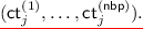
• $\mathsf {Test}(\mathsf {ct}[1], \ldots , \mathsf {ct}[\lambda ], \ldots , \mathsf {ct}[|\mathsf {sk}|] ) \rightarrow \{0,1\}$. The testing algorithm takes as input a sequence of $|\mathsf {sk}|$ ciphertexts $(\mathsf {ct}[1], \ldots , \mathsf {ct}[\lambda ], \ldots )$. We will assume the algorithm also knows the LWE modulus q. It parses the first $\lambda$ ciphertexts as $\mathsf {ct}[k] = \left( \left\{ \varvec{\mathrm {B}}^{(i)}_{0, 1}\right\} _i, \left\{ \mathsf {ct}[k]^{(i)}_j\right\} _{i, j} \right)$ for $k \le \lambda$. Next, it computes the following

  $$ \mathsf {sum} = \sum _{i = 1}^{\mathsf {nbp}} \varvec{\mathrm {B}}^{(i)}_{0, 1} \cdot \prod _{j = 1}^{L} \mathsf {ct}[\mathsf {inp}(j)]^{(i)}_j. $$

  If each component of $\mathsf {sum}$ lies in $\left( -q/4, q/4 \right)$, then the algorithm outputs 1 to indicate a cycle. Otherwise it outputs 0. We would like to remind the reader that the starting state $\mathsf {st}_0$ of each branching program $\mathsf {BP}^{(i)}$ is 1 (assumed w.l.o.g. in Sect. 2.2), therefore the testing algorithm only requires the matrices $\varvec{\mathrm {B}}^{(i)}_{0, 1}$ to start oblivious evaluation of each branching program.

Fig. 2.

Routine $\mathsf {SubEncrypt}$

4.2 Proof of Correctness

In this section, we will prove correctness of our bit-encryption cycle tester. Concretely, we show that the $\mathsf {Test}$ algorithm distinguishes between a sequence of $|\mathsf {sk}|$ ciphertexts where $k^{th}$ ciphertext encrypts $k^{th}$ bit of the secret key, and a sequence of encryptions of zeros with non-negligible probability. First, we show that if $\mathsf {Test}$ algorithm is given encryptions of secret key bits, then it outputs 1 with all-but-negligible probability. Next, we show that if $\mathsf {Test}$ algorithm is run on encryptions of zeros, then it outputs 0 with all-but-negligible probability. Using these two facts, correctness of our cycle tester follows.

Testing Encryptions of Key Bits. Let $\varvec{\mathrm {ct}} = (\mathsf {ct}[1], \ldots , \mathsf {ct}[\lambda ], \ldots )$ be the sequence of $|\mathsf {sk}|$ ciphertexts where $k^{th}$ ciphertext encrypts bit $\mathsf {sk}_k$, and it can be parsed as $\mathsf {ct}[k] = \left( \left\{ \varvec{\mathrm {B}}^{(i)}_{0, 1}\right\} _i, \left\{ \mathsf {ct}[k]^{(i)}_j\right\} _{i, j} \right)$. Recall that the first $\lambda$ bits of secret key $\mathsf {sk}$ correspond to the PRF key s. Therefore, $\mathsf {ct}[k]$ is an encryption of the bit $s_k$ for $k \le \lambda$. Also, $i^{th}$ branching program $\mathsf {BP}^{(i)}$ computes the function $\mathrm {PRF}_\lambda (\cdot , i)$. This could be equivalently stated as

$$ \forall \ i \le \mathsf {nbp}, \qquad \sigma ^{(i)}_{L, b_L}\left( \cdots \left( \sigma ^{(i)}_{1, b_1} (1) \right) \cdots \right) = {\left\{ \begin{array}{ll} \mathsf {rej}^{(i)}&{} \text { if } \mathrm {PRF}(s, i) = 0, \\ \mathsf {acc}^{(i)}&{} \text { if } \mathrm {PRF}(s, i) = 1 \end{array}\right. } $$

where $b_j = s_{\mathsf {inp}(j)}$ for $j \le L$. Let $\mathsf {st}^{(i)}_j$ denote the state of the $i^{th}$ branching program after j steps. The initial state $\mathsf {st}^{(i)}_{0}$ is 1 for all programs, and $j^{th}$ state can be computed as $\mathsf {st}^{(i)}_j= \sigma ^{(i)}_{j, s_{\mathsf {inp}(j)}} (\mathsf {st}^{(i)}_{j - 1})$.

Note that every ciphertext $\mathsf {ct}[k]$ consists of L sub-ciphertexts $\mathsf {ct}[k]_j$ for each level $j \le L$, and each sub-ciphertext consists of $\mathsf {nbp}$ short matrices, each for a separate branching program. For constructing each sub-ciphertext, exactly one short secret matrix $\varvec{\mathrm {S}}_j$ is chosen, and it is shared across all $\mathsf {nbp}$ branching programs for generating LWE-type samples. It is crucial for testability that $\varvec{\mathrm {S}}_j$’s stay same for all branching programs.

First, we will introduce some notations for this proof.

• $\varvec{\mathrm {S}}[k]_j$: matrix chosen at level j for computing $\mathsf {ct}[k]^{(i)}_j$

• $\varvec{\mathrm {E}}[k]^{(i)}_{j}$: error matrix chosen at level j, program i for computing $\mathsf {ct}[k]^{(i)}_j$

• $\mathsf {inp}_j= \mathsf {inp}(j)$: the input bit read at level j of the branching program

• $\varvec{\mathrm {S}}_j= \varvec{\mathrm {S}}[\mathsf {inp}_j]_j$, $\varvec{\mathrm {E}}^{(i)}_j= \varvec{\mathrm {E}}[\mathsf {inp}_j]^{(i)}_{j}$, $\mathsf {CT}^{(i)}_j= \mathsf {ct}[\mathsf {inp}_j]^{(i)}_j$

• $\mathbf {\Gamma }_{j^{*}}= \prod _{j = 1}^{j^{*}} \varvec{\mathrm {S}}_j$

• $\varvec{\mathrm {\Delta }}^{(i)}_{j^{*}}= \varvec{\mathrm {B}}^{(i)}_{0, 1} \cdot \left( \prod _{j = 1}^{j^{*}} \mathsf {CT}^{(i)}_j \right)$,    $\widetilde{\varvec{\mathrm {\Delta }}}^{(i)}_{j^{*}}= \mathbf {\Gamma }_{j^{*}}\cdot \varvec{\mathrm {B}}^{(i)}_{j^{*}, \mathsf {st}^{(i)}_{j^{*}}}$,    $\varvec{\mathrm {Err}}^{(i)}_{j^{*}}= \varvec{\mathrm {\Delta }}^{(i)}_{j^{*}}- \widetilde{\varvec{\mathrm {\Delta }}}^{(i)}_{j^{*}}$.

The $\mathsf {Test}$ algorithm checks that $\left\| {\sum _{i = 1}^{\mathsf {nbp}} \varvec{\mathrm {\Delta }}^{(i)}_{L}}\right\| _\infty < q/4$. Also, note that

$$ \sum _{i = 1}^{\mathsf {nbp}} \widetilde{\varvec{\mathrm {\Delta }}}^{(i)}_{L} = \sum _{i = 1}^{\mathsf {nbp}} \mathbf {\Gamma }_{L} \cdot \varvec{\mathrm {B}}^{(i)}_{L, \mathsf {st}^{(i)}_{L}} = \mathbf {\Gamma }_{L} \cdot \sum _{i = 1}^{\mathsf {nbp}} \varvec{\mathrm {B}}^{(i)}_{L, \mathsf {st}^{(i)}_{L}} = \varvec{\mathrm {0}}. $$

Thus, it would be sufficient to show that, with high probability, $\varvec{\mathrm {Err}}^{(i)}_{L}= {\varvec{\mathrm {\Delta }}^{(i)}_{L} - \widetilde{\varvec{\mathrm {\Delta }}}^{(i)}_{L}}$ is bounded. We will show that for all $i\le \mathsf {nbp}$, $j^{*}\le L$, $\varvec{\mathrm {Err}}^{(i)}_{j^{*}}$ is bounded.

Lemma 2

$\forall \ i \in \left\{ 1, \ldots , \mathsf {nbp}\right\} , {j^{*}\in \left\{ 1, \ldots , L\right\} }{,} \quad \left\| {\varvec{\mathrm {Err}}^{(i)}_{j^{*}}}\right\| _\infty \le j^{*}\cdot \left( m \cdot \sigma \right) ^{j^{*}}$ with overwhelming probability.

Proof

The above lemma is proven by induction over $j^{*}$, and all arguments hold irrespective of the value of i. Therefore, for simplicity of notation, we will drop the dependence on i. We will slightly abuse the notation and use $\varvec{\mathrm {B}}^{(i)}_{j, \sigma ^{(i)}_{j, m}}$ to denote the following matrix.

$$ \varvec{\mathrm {B}}^{(i)}_{j, \sigma ^{(i)}_{j, m}} = \begin{bmatrix} \varvec{\mathrm {B}}^{(i)}_{j, \sigma ^{(i)}_{j, m}(1)} \\ \vdots \\ \varvec{\mathrm {B}}^{(i)}_{j, \sigma ^{(i)}_{j, m}(w)} \end{bmatrix}. $$

Before proceeding to our inductive proof, we would like to note the following fact.

Fact 1

For all $j \le L$, $\mathsf {CT}^{(i)}_j\leftarrow \mathsf {SamplePre}(\varvec{\mathrm {B}}^{(i)}_{j - 1}, T^{(i)}_{j - 1}, \sigma , \varvec{\mathrm {C}}^{(i)}_{j})$, where $\varvec{\mathrm {C}}^{(i)}_{j} = \left( \varvec{\mathrm {I}}_w \otimes \varvec{\mathrm {S}}_j \right) \cdot \varvec{\mathrm {B}}^{(i)}_{j, \sigma ^{(i)}_{j, m}} + \varvec{\mathrm {E}}^{(i)}_j$ and $m = s_{\mathsf {inp}_j}$.

Base case $(j^{*}= 1){ .}$ We know that $\varvec{\mathrm {\Delta }}_{1} = \varvec{\mathrm {B}}_{0, 1} \cdot \left( \mathsf {CT}_{1} \right)$. Therefore, using Fact 1, we can say that $\varvec{\mathrm {\Delta }}_{1} = \varvec{\mathrm {S}}_{1} \cdot \varvec{\mathrm {B}}_{1, \mathsf {st}_{1}} + \varvec{\mathrm {E}}_{1, 1} = \widetilde{\varvec{\mathrm {\Delta }}}_{1} + \varvec{\mathrm {E}}_{1, 1}$. Note that $\varvec{\mathrm {E}}_{1, 1}$ is an $n \times m$ submatrix consisting of first n rows of $\varvec{\mathrm {E}}_{1}$. Thus, we could write the following

$$ \left\| {\varvec{\mathrm {Err}}_{1}}\right\| _\infty = \left\| {\varvec{\mathrm {\Delta }}_{1} - \widetilde{\varvec{\mathrm {\Delta }}}_{1}}\right\| _\infty = \left\| {\varvec{\mathrm {E}}_{1, 1}}\right\| _\infty \le m \cdot \sigma . $$

This completes the proof of base case. For the induction step, we assume that the above lemma holds for $j^{*}- 1$, and show that it holds for $j^{*}$ as well.

Induction Step. We know that $\varvec{\mathrm {\Delta }}_{j^{*}} = \varvec{\mathrm {\Delta }}_{j^{*}- 1} \cdot \left( \mathsf {CT}_{j^{*}} \right)$. Also, $\varvec{\mathrm {\Delta }}_{j^{*}- 1} = \widetilde{\varvec{\mathrm {\Delta }}}_{j^{*}- 1} + \varvec{\mathrm {Err}}_{j^{*}- 1}$. So, we could write the following

$$\begin{aligned} \varvec{\mathrm {\Delta }}_{j^{*}}&= \widetilde{\varvec{\mathrm {\Delta }}}_{j^{*}- 1} \cdot {\mathsf {CT}_{j^{*}}} + \varvec{\mathrm {Err}}_{j^{*}- 1} \cdot {\mathsf {CT}_{j^{*}}} \\&= \mathbf {\Gamma }_{j^{*}-1} \cdot \left( \varvec{\mathrm {B}}_{j^{*}- 1, \mathsf {st}_{j^{*}- 1}} \cdot \mathsf {CT}_{j^{*}} \right) + \varvec{\mathrm {Err}}_{j^{*}- 1} \cdot \mathsf {CT}_{j^{*}} \\&= \mathbf {\Gamma }_{j^{*}-1} \cdot \left( \varvec{\mathrm {S}}_{j^{*}} \cdot \varvec{\mathrm {B}}_{j^{*}, \mathsf {st}_{j^{*}}} + \varvec{\mathrm {E}}_{j^{*}, \mathsf {st}_{j^{*}- 1}} \right) + \varvec{\mathrm {Err}}_{j^{*}- 1} \cdot \mathsf {CT}_{j^{*}} \\&= \widetilde{\varvec{\mathrm {\Delta }}}^{(i)}_{j^{*}} + \mathbf {\Gamma }_{j^{*}-1} \cdot \varvec{\mathrm {E}}_{j^{*}, \mathsf {st}_{j^{*}- 1}} + \varvec{\mathrm {Err}}_{j^{*}- 1} \cdot \mathsf {CT}_{j^{*}} \end{aligned}$$

Here, $\varvec{\mathrm {E}}_{j^{*}, \mathsf {st}_{j^{*}- 1}}$ is an $n \times m$ submatrix of $\varvec{\mathrm {E}}_{j^{*}}$. Finally, we can bound $\varvec{\mathrm {Err}}_{j^{*}}$ as follows

$$\begin{aligned} \left\| {\varvec{\mathrm {Err}}_{j^{*}}}\right\| _\infty&= \left\| {\varvec{\mathrm {\Delta }}_{j^{*}} - \widetilde{\varvec{\mathrm {\Delta }}}_{j^{*}}}\right\| _\infty = \left\| {\mathbf {\Gamma }_{j^{*}-1} \cdot \varvec{\mathrm {E}}_{j^{*}, \mathsf {st}_{j^{*}- 1}} + \varvec{\mathrm {Err}}_{j^{*}- 1} \cdot \mathsf {CT}_{j^{*}}}\right\| _\infty \\&\le \left\| {\mathbf {\Gamma }_{j^{*}-1} \cdot \varvec{\mathrm {E}}_{j^{*}, \mathsf {st}_{j^{*}- 1}}}\right\| _\infty + \left\| {\varvec{\mathrm {Err}}_{j^{*}- 1} \cdot \mathsf {CT}_{j^{*}}}\right\| _\infty \\&\le \left( n \cdot \sigma \right) ^{j^{*}- 1} \cdot m \cdot \sigma + (j^{*}- 1) \cdot (m \cdot \sigma )^{j^{*}- 1} \cdot m \cdot \sigma \le j^{*}\cdot (m \cdot \sigma )^{j^{*}} \end{aligned}$$

This completes the proof.

Using Lemma 2, we can claim that for all $i \le \mathsf {nbp}$, $\left\| {\varvec{\mathrm {\Delta }}^{(i)}_{L} - \widetilde{\varvec{\mathrm {\Delta }}}^{(i)}_{L}}\right\| _\infty \le L \cdot \left( m \cdot \sigma \right) ^{L}$. Therefore,

$$\begin{aligned} \left\| {\mathsf {sum}}\right\| _\infty&= \left\| {\sum _{i = 1}^{\mathsf {nbp}} \varvec{\mathrm {\Delta }}^{(i)}_{L}}\right\| _\infty = \left\| {\sum _{i = 1}^{\mathsf {nbp}} \varvec{\mathrm {\Delta }}^{(i)}_{L} - \sum _{i = 1}^{\mathsf {nbp}} \widetilde{\varvec{\mathrm {\Delta }}}^{(i)}_{L}}\right\| _\infty \le \mathsf {nbp}\cdot L \cdot \left( m \cdot \sigma \right) ^{L} < q/4 \end{aligned}$$

Therefore, for our setting of parameters, if ciphertexts encrypt the secret key bit-by-bit, then $\mathsf {Test}$ algorithm outputs 1 with high probability.

Testing Encryptions of Zeros

Lemma 3

If $\mathrm {PRF}$ is a family of secure pseudorandom functions and challenge ciphertexts are encryptions of zeros, then $\mathsf {Test}$ outputs 0 with all-but-negligible probability.

Proof

Since the ciphertexts are encryptions of zeros, each branching program $\mathsf {BP}^{(i)}$ computes the value $t_i' = \mathrm {PRF}_\lambda (0, i)$. Also, with high probability, $t_i'$ and $t_i$ can not be equal for all $i \le \lambda$ as otherwise $\mathrm {PRF}_\lambda$ will not be a secure pseudorandom function. Therefore, with high probability,

$$ \widetilde{\mathsf {sum}} = \sum _{i = 1}^{\mathsf {nbp}} \widetilde{\varvec{\mathrm {\Delta }}}^{(i)}_{L} = \left( \prod _{j = 1}^{L} \varvec{\mathrm {S}}_j \right) \cdot \sum _{i = 1}^{\mathsf {nbp}} \varvec{\mathrm {B}}^{(i)}_{L, \mathsf {st}^{(i)}_{L}} \ne \varvec{\mathrm {0}}. $$

Now, $\sum _{i = 1}^{\mathsf {nbp}} \varvec{\mathrm {B}}^{(i)}_{L, \mathsf {st}^{(i)}_{L}}$ will be a uniformly random matrix in $\mathbb {Z}_q^{n \times m}$ as $t' \ne t$ and $\varvec{\mathrm {B}}^{(i)}_{L, \mathsf {st}^{(i)}_{L}}$ are randomly chosen for $i \le \mathsf {nbp}$. Let $\varvec{\mathrm {S}}$ denote the product $\prod _{j = 1}^{L} \varvec{\mathrm {S}}_j$ and $\varvec{\mathrm {B}}$ denote the sum $\sum _{i = 1}^{\mathsf {nbp}} \varvec{\mathrm {B}}^{(i)}_{L, \mathsf {st}^{(i)}_{L}}$. We can write $\widetilde{\mathsf {sum}}$ as $\widetilde{\mathsf {sum}} = \varvec{\mathrm {S}} \cdot \varvec{\mathrm {B}}$, where $\varvec{\mathrm {B}}$ is a random $n \times m$ matrix. Thus, $\widetilde{\mathsf {sum}}$ is a random $n \times m$ matrix as $\varvec{\mathrm {S}}$, product of L full rank matrices, is also full rank. So, with high probability, at least one entry in matrix $\mathsf {sum}$ will have absolute value $> q/4$ which implies that $\mathsf {Test}$ outputs 0.

4.3 IND-CPA Proof

We will now show that the construction described above is ${\mathsf{IND}}{\text {-}}{\mathsf{CPA}}$ secure. The adversary queries for ciphertexts, and each ciphertext consists of $L\cdot \mathsf {nbp}$ sub-sub-ciphertexts. In our proof, we will gradually switch the sub-sub-ciphertexts to random low-norm (Gaussian) matrices, starting with the top-level sub-ciphertext and moving down. Once all sub-ciphertexts are switched to Gaussian matrices, the adversary has no information about the challenge message.

Our proof proceeds via a sequence of hybrid games. First, we switch the PRF evaluation to a truly random $\mathsf {nbp}$ bit string. Next, we switch the top level matrices to truly random matrices. This is possible since $\mathsf {nbp}$ is much larger than n, m, and as a result, we can use Leftover Hash Lemma. Once all top level matrices are truly random, we can make the top-level sub-sub-ciphertexts to be random low norm (Gaussian) matrices. This follows from the LWE security, together with the Property 3 of lattice trapdoors. Once the top level sub-sub-ciphertexts are Gaussian, we do not require the trapdoors at level $L-1$. As a result, we can choose uniformly random matrices at level $L-1$. This will allow us to switch the sub-sub-ciphertexts at level $L-1$ to Gaussian matrices. Proceeding this way, we can switch all sub-sub-ciphertexts to Gaussian matrices.

We will first define the sequence of hybrid games, and then show that they are computationally indistinguishable. The first hybrid corresponds to the original security game. In the subsequent hybrids, we only show the steps that are modified.

Sequence of Hybrid Games

$\mathsf {Game} ~0$: This corresponds to the original security game.

• Setup Phase

  • 1. The challenger first chooses the LWE parameters n, m, q, $\sigma$, $\chi$ and $\mathsf {nbp}$. Recall $L = {\ell }{\text {-}}\mathsf{bp}(\lambda )$ and $w = \mathsf{w}{\text {-}}\mathsf{bp}(\lambda )$.

  • 2. Next, it chooses a uniformly random string $s \leftarrow \{0,1\}^\lambda$ and sets $t_i = \mathrm {PRF}(s, i)$ for $i\le \mathsf {nbp}$.

  • 3. For $i = 1$ to $\mathsf {nbp}$ and $j = 0$ to $L - 1$, it chooses $(\varvec{\mathrm {B}}^{(i)}_j, T^{(i)}_j) \leftarrow \mathsf {TrapGen}(1^{w\cdot n}, 1^m, q)$.

  • 4. It chooses $\mathsf {nbp}$ uniformly random matrices $\varvec{\mathrm {B}}^{(i)}_L$ of dimensions $w\cdot n \times m$, such that the following constraint is satisfied

    $$ \sum _{i\ :\ t_i = 0} \varvec{\mathrm {B}}^{(i)}_{L, \mathsf {rej}^{(i)}} + \sum _{i\ :\ t_i = 1} \varvec{\mathrm {B}}^{(i)}_{L, \mathsf {acc}^{(i)}} = \varvec{\mathrm {0}}. $$

  • 5. Finally, the challenger sets $\mathsf {sk}= \left( s, \left\{ \varvec{\mathrm {B}}^{(i)}_j, T^{(i)}_j\right\} _{i, j} \right)$.

• Pre-Challenge Query Phase

  • 1. The adversary requests polynomially many encryption queries. The challenger responds to each encryption query as follows.

    For $j=1$ to L, the challenger computes $\mathsf {ct}_j \leftarrow \mathsf {SubEncrypt}(\mathsf {sk}, m, j)$ and sends $\mathsf {ct}= \left( \left\{ \varvec{\mathrm {B}}^{(i)}_{0, 1}\right\} _i, (\mathsf {ct}_1, \ldots , \mathsf {ct}_L) \right)$.

• Challenge Phase. The challenger chooses a bit $b \leftarrow \{0,1\}$, and computes the challenge ciphertext identical to any pre-challenge query ciphertext for bit b.

• Post-Challenge Query Phase. This is identical to the pre-challenge query phase.

• Guess. The adversary finally sends the guess $b'$, and wins if $b=b'$.

$\mathsf {Game} ~1$: This hybrid experiment is similar to the previous one, except that the string $t = (t_1, \ldots , t_\mathsf {nbp})$ is a uniformly random $\mathsf {nbp}$ bit string. Also, in place of the PRF key in the secret key, we have an empty string $\perp$. Note that this does not affect the encryption algorithm since it works oblivious to the PRF key (the PRF key is not used during encryption).

• Setup Phase

  • 1. The challenger first chooses the LWE parameters n, m, q, $\sigma$, $\chi$ and $\mathsf {nbp}$. Recall $L = {\ell }{\text {-}}\mathsf{bp}(\lambda )$ and $w = \mathsf{w}{\text {-}}\mathsf{bp}(\lambda )$.

  • 2. .

  • 3. For $i = 1$ to $\mathsf {nbp}$ and $j = 0$ to $L - 1$, it chooses $(\varvec{\mathrm {B}}^{(i)}_j, T^{(i)}_j) \leftarrow \mathsf {TrapGen}(1^{w\cdot n}, 1^m, q)$.

  • 4. It chooses $\mathsf {nbp}$ uniformly random matrices $\varvec{\mathrm {B}}^{(i)}_L$ of dimensions $w\cdot n \times m$, such that the following constraint is satisfied

    $$ \sum _{i\ :\ t_i = 0} \varvec{\mathrm {B}}^{(i)}_{L, \mathsf {rej}^{(i)}} + \sum _{i\ :\ t_i = 1} \varvec{\mathrm {B}}^{(i)}_{L, \mathsf {acc}^{(i)}} = \varvec{\mathrm {0}}. $$

  • 5. Finally, the challenger sets $\mathsf {sk}= \left( \perp , \left\{ \varvec{\mathrm {B}}^{(i)}_j, T^{(i)}_j\right\} _{i, j} \right)$.

$\mathsf {Game} ~2$: In this hybrid experiment, the challenger chooses the top-level matrices $\varvec{\mathrm {B}}^{(i)}_L$ uniformly at random.

• Setup Phase

  • 1. The challenger first chooses the LWE parameters n, m, q, $\sigma$, $\chi$ and $\mathsf {nbp}$. Recall $L = {\ell }{\text {-}}\mathsf{bp}(\lambda )$ and $w = \mathsf{w}{\text {-}}\mathsf{bp}(\lambda )$.

  • 2. Next, it chooses $t \leftarrow \{0,1\}^\mathsf {nbp}$.

  • 3. For $i = 1$ to $\mathsf {nbp}$ and $j = 0$ to $L - 1$, it chooses $(\varvec{\mathrm {B}}^{(i)}_j, T^{(i)}_j) \leftarrow \mathsf {TrapGen}(1^{w\cdot n}, 1^m, q)$.

  • 4. .

  • 5. Finally, the challenger sets $\mathsf {sk}= \left( \perp , \left\{ \varvec{\mathrm {B}}^{(i)}_j, T^{(i)}_j\right\} _{i, j} \right)$.

Next, we have a sequence of 3L hybrid experiments $\mathsf {Game} ~2.\mathsf {level}.\left\{ 1, 2, 3\right\}$ for $\mathsf {level}= L$ to 1.

$\mathsf {Game} ~2.\mathsf {level}.1$: In hybrids $\mathsf {Game} ~2.\mathsf {level}.1$, the sub-ciphertexts corresponding to levels greater than $\mathsf {level}$ are Gaussian matrices. At level $\mathsf {level}$, the sub-ciphertext computation does not use $\mathsf {SubEncrypt}$ routine. Instead, it chooses a uniformly random matrix and computes the $\mathsf {SamplePre}$ of the uniformly random matrix. Also, for levels greater than $\mathsf {level}- 1$, matrices $\varvec{\mathrm {B}}^{(i)}_j$ are chosen uniformly at random instead of being sampled using $\mathsf {TrapGen}$.

• Pre-Challenge Query Phase

  • 1. The adversary requests polynomially many encryption queries. The challenger responds to each encryption query as follows.

  • 2. For $j = 1$ to $\mathsf {level}- 1$, the challenger computes $\mathsf {ct}_j \leftarrow \mathsf {SubEncrypt}(\mathsf {sk}, m, j)$.

  • 3.

  • 4. For $i = 1$ to $\mathsf {nbp}$ and $j = \mathsf {level}+ 1$ to L, the challenger chooses $\mathsf {ct}^{(i)}_j\leftarrow \chi ^{m \times m}$. It sets $\mathsf {ct}_j = (\mathsf {ct}^{(1)}_j, \ldots , \mathsf {ct}^{(\mathsf {nbp})}_j)$.

  • 5. Finally, it sets $\mathsf {ct}= \left( \left\{ \varvec{\mathrm {B}}^{(i)}_{0, 1}\right\} _i, (\mathsf {ct}_1, \ldots , \mathsf {ct}_L) \right)$ and sends $\mathsf {ct}$ to the adversary.

$\mathsf {Game} ~2.\mathsf {level}.2$: In hybrids $\mathsf {Game} ~2.\mathsf {level}.2$, the sub-ciphertexts corresponding to levels greater than $\mathsf {level}- 1$ are Gaussian matrices.

• Pre-Challenge Query Phase

  • 1. The adversary requests polynomially many encryption queries. The challenger responds to each encryption query as follows.

  • 2. For $j = 1$ to $\mathsf {level}- 1$, the challenger computes $\mathsf {ct}_j \leftarrow \mathsf {SubEncrypt}(\mathsf {sk}, m, j)$.

  • 3.

  • 4. Finally, it sets $\mathsf {ct}= \left( \left\{ \varvec{\mathrm {B}}^{(i)}_{0, 1}\right\} _i, (\mathsf {ct}_1, \ldots , \mathsf {ct}_L) \right)$ and sends $\mathsf {ct}$ to the adversary.

$\mathsf {Game} ~2.\mathsf {level}.3$: In hybrids $\mathsf {Game} ~2.\mathsf {level}.3$, matrices $\varvec{\mathrm {B}}^{(i)}_j$ are chosen uniformly at random instead of being sampled using $\mathsf {TrapGen}$ for levels greater than $\mathsf {level}- 2$.

• Setup Phase

  • 1. The challenger first chooses the LWE parameters n, m, q, $\sigma$, $\chi$ and $\mathsf {nbp}$. Recall $L = {\ell }{\text {-}}\mathsf{bp}(\lambda )$ and $w = \mathsf{w}{\text {-}}\mathsf{bp}(\lambda )$.

  • 2. Next, it chooses $t \leftarrow \{0,1\}^\mathsf {nbp}$.

  • 3. For $i = 1$ to $\mathsf {nbp}$ and $j = 0$ to $\mathsf {level}- 2$, it chooses $(\varvec{\mathrm {B}}^{(i)}_j, T^{(i)}_j) \leftarrow \mathsf {TrapGen}(1^{w\cdot n}, 1^m, q)$.

  • 4.

  • 5. Finally, the challenger sets $\mathsf {sk}= \left( \perp , \left\{ \varvec{\mathrm {B}}^{(i)}_j, T^{(i)}_j\right\} _{i, j} \right)$.

Indistinguishability of Hybrid Games. We now establish via a sequence of lemmas that no PPT adversary can distinguish between any two adjacent games with non-negligible advantage. To conclude, we show that the advantage of any PPT adversary in the last game is 0.

Let $\mathcal {A}$ be a PPT adversary that breaks the security of our construction in the IND-CPA security game (Definition 4). In $\mathsf {Game} ~i$, advantage of $\mathcal {A}$ is defined as $\mathsf {Adv}_\mathcal {A}^i = |\Pr [\mathcal {A}\text { wins}] - 1/2|$. We show via a sequence of claims that $\mathcal {A}$’s advantage is distinguishing between any two consecutive games must be negligible, otherwise there will be a poly-time attack on the security of some underlying primitive. Finally, in last game, we show that $\mathcal {A}$’s advantage in the last game is 0.

Lemma 4

If $\mathrm {PRF}$ is a family of secure pseudorandom functions, then for any PPT adversary $\mathcal {A}$, $|\mathsf {Adv}^0_\mathcal {A}- \mathsf {Adv}^1_\mathcal {A}| \le negl(\lambda )$ for some negligible function $negl(\cdot )$.

Proof

We describe a reduction algorithm $\mathcal {B}$ which plays the indistinguishability based game with $\mathrm {PRF}$ challenger. $\mathcal {B}$ runs the Setup Phase as in $\mathsf {Game}$ 0, except it does not choose a string $s \leftarrow \{0, 1\}^{\lambda }$. $\mathcal {B}$ makes $\mathsf {nbp}$ queries to the $\mathrm {PRF}$ challenger, where in the $i^{th}$ query it sends i to the $\mathrm {PRF}$ challenger and sets $t_i$ as the challenger’s response. $\mathcal {B}$ performs remaining steps as in $\mathsf {Game}$ 0, and sends 1 to the $\mathrm {PRF}$ challenger if $\mathcal {A}$ guesses the bit correctly, otherwise it sends 0 to the $\mathrm {PRF}$ challenger as its guess.

Note that when $\mathrm {PRF}$ challenger honestly evaluates the $\mathrm {PRF}$ on each query, then $\mathcal {B}$ exactly simulates the view of $\mathsf {Game}$ 0 for $\mathcal {A}$. Otherwise if $\mathrm {PRF}$ challenger behaves as a random function, then $\mathcal {B}$ exactly simulates the view of $\mathsf {Game}$ 1. Therefore, if $|\mathsf {Adv}^0_\mathcal {A}- \mathsf {Adv}^1_\mathcal {A}|$ is non-negligible, then $\mathrm {PRF}$ is not secure pseudorandom function family.

Lemma 5

For any adversary $\mathcal {A}$, $|\mathsf {Adv}^1_\mathcal {A}- \mathsf {Adv}^2_\mathcal {A}| \le negl(\lambda )$ for some negligible function $negl(\cdot )$.

Proof

The proof of this lemma follows from Corollary 1 which itself follows from the Leftover Hash Lemma Theorem 1. Note that the difference between $\mathsf {Game}$ 1 and 2 is the way top level matrices $\varvec{\mathrm {B}}^{(i)}_L$ are sampled during Setup Phase. In $\mathsf {Game}$ 1, matrix $\varvec{\mathrm {B}}^{(\mathsf {nbp})}_{L, \mathsf {st}^{(i)}_L}$ is chosen as

$$ \varvec{\mathrm {B}}^{(\mathsf {nbp})}_{L, \mathsf {st}^{(\mathsf {nbp})}_L} = -\, \left( \sum _{i \le \mathsf {nbp}- 1\ :\ t_i = 0} \varvec{\mathrm {B}}^{(i)}_{L, \mathsf {rej}^{(i)}} + \sum _{i \le \mathsf {nbp}- 1\ :\ t_i = 1} \varvec{\mathrm {B}}^{(i)}_{L, \mathsf {acc}^{(i)}} \right) , $$

where $\mathsf {st}^{(\mathsf {nbp})}_L$ is $\mathsf {acc}^{(\mathsf {nbp})}$ if $t_\mathsf {nbp}= 1$, and $\mathsf {rej}^{(\mathsf {nbp})}$ otherwise. It can be equivalently written as follows

$$ \varvec{\mathrm {B}}^{(\mathsf {nbp})}_{L, \mathsf {st}_L^{(\mathsf {nbp})}} = - \varvec{\mathrm {A}} \cdot \varvec{\mathrm {R}}, \qquad \varvec{\mathrm {A}} = \begin{bmatrix} \varvec{\mathrm {B}}^{(1)}_{L, \mathsf {rej}^{(1)}} \left| \right| \varvec{\mathrm {B}}^{(1)}_{L, \mathsf {acc}^{(1)}} \left| \right| \dots {\left| \right| } \varvec{\mathrm {B}}^{(\mathsf {nbp}- 1)}_{L, \mathsf {rej}^{(\mathsf {nbp}- 1)}} \left| \right| \varvec{\mathrm {B}}^{(\mathsf {nbp}- 1)}_{L, \mathsf {acc}^{(\mathsf {nbp}- 1)}} \end{bmatrix} $$

where $\varvec{\mathrm {R}} = \varvec{\mathrm {u}} \otimes \varvec{\mathrm {I}}_m \in \mathbb {Z}_q^{2 m (\mathsf {nbp}- 1) \times m}$, $\varvec{\mathrm {u}} = (u_1, \ldots , u_{2 \mathsf {nbp}- 2})^{\top }\in \{0, 1\}^{2 \mathsf {nbp}- 2}$ and for all $i \le \mathsf {nbp}- 1$, $u_{2 i} = t_i$ and $u_{2 i - 1} = 1 - t_i$. That is, matrix $\varvec{\mathrm {R}}$ consists of $2 \mathsf {nbp}- 2$ submatrices where if $t_i = 1$, then its $2 i^{th}$ submatrix is identity and $(2 i - 1)^{th}$ submatrix is zero, otherwise it is the opposite. Let $\mathcal {R}$ denote the distribution of matrix $\varvec{\mathrm {R}}$ as described above with t drawn uniformly from $\{0, 1\}^{\mathsf {nbp}}$. Note that $\varvec{\mathrm {H}}_\infty (\mathcal {R}) = \mathsf {nbp}- 1$ (min-entropy of $\mathcal {R}$), and $\mathsf {nbp}> m \cdot n \log _2 q + \omega (\log n)$. Therefore, it follows (from Corollary 1) that

Thus, $|\mathsf {Adv}^1_\mathcal {A}- \mathsf {Adv}^2_\mathcal {A}|$ is negligible in the security parameter for all PPT adversaries $\mathcal {A}$.

Lemma 6

If $(n, \mathsf {nbp}\cdot w \cdot m, q, \chi ){\text {-}}\mathsf {LWE}{\text {-}}\mathsf {ss}$ assumption holds (Assumption 2), then for any PPT adversary $\mathcal {A}$, $|\mathsf {Adv}^2_\mathcal {A}- \mathsf {Adv}^{2.L.1}_\mathcal {A}| \le negl(\lambda )$ for some negligible function $negl(\cdot )$.

Proof

The difference between $\mathsf {Game}$ 2 and 2.L.1 is the way top-level sub-ciphertexts ($\mathsf {ct}_L$) are created for all encryption queries (including challenge query). Recall that $\mathsf {ct}_L$ contains $\mathsf {nbp}$ short matrices $\mathsf {ct}^{(i)}_L$, and each $\mathsf {ct}^{(i)}_L$ is sampled as $\mathsf {ct}^{(i)}_L\leftarrow \mathsf {SamplePre}(\varvec{\mathrm {B}}^{(i)}_{L - 1}, T^{(i)}_{L - 1}, \sigma , \varvec{\mathrm {C}}^{(i)}_L)$. In $\mathsf {Game}$ 2, matrix $\varvec{\mathrm {C}}^{(i)}_L$ is computed as $\varvec{\mathrm {C}}^{(i)}_L = \left( \varvec{\mathrm {I}}_w \otimes \varvec{\mathrm {S}}_L \right) \cdot \varvec{\mathrm {D}}^{(i)}_L + \varvec{\mathrm {E}}^{(i)}_L$, where $\varvec{\mathrm {D}}^{(i)}_L$ is a permutation of $\varvec{\mathrm {B}}^{(i)}_L$ and $\varvec{\mathrm {E}}^{(i)}_L$ is chosen as $\varvec{\mathrm {E}}^{(i)}_L \leftarrow \chi ^{w\cdot n \times m}$. On the other hand, in $\mathsf {Game}$ 2.L.1, it is chosen as $\varvec{\mathrm {C}}^{(i)}_L \leftarrow \mathbb {Z}_q^{w\cdot n \times m}$.

For proving indistinguishability of $\mathsf {Game}$ 2 and 2.L.1, we need to sketch q intermediate hybrids, where q is the total number of queries made by $\mathcal {A}$.⁷ In $k^{th}$ hybrid, the challenger proceeds as $\mathsf {Game}$ 2.L.1 while answering first k queries, and proceeds as in $\mathsf {Game}$ 2 for answering remaining queries. Indistinguishability between any two consecutive intermediate hybrids follows directly from $\mathsf {LWE}{\text {-}}\mathsf {ss}$ assumption. Below we describe a reduction algorithm $\mathcal {B}$ which plays the $\mathsf {LWE}{\text {-}}\mathsf {ss}$ indistinguishability game.

First, $\mathcal {B}$ receives as $\mathsf {LWE}{\text {-}}\mathsf {ss}$ challenge two $n \times (\mathsf {nbp}\cdot w \cdot m)$ matrices $(\varvec{\mathrm {F}}, \varvec{\mathrm {G}})$. It parses $\varvec{\mathrm {F}}$ into $\mathsf {nbp}$ submatrices of dimensions $n \times (w \cdot m)$ as $[\varvec{\mathrm {F}}^{(1)} \left| \right| \dots \left| \right| \varvec{\mathrm {F}}^{(\mathsf {nbp})}] = \varvec{\mathrm {F}}$. Further, each matrix $\varvec{\mathrm {F}}^{(i)}$ is parsed into w matrices of dimensions $n \times m$ as $[\varvec{\mathrm {F}}^{(i)}_1 \left| \right| \dots \left| \right| \varvec{\mathrm {F}}^{(i)}_w] = \varvec{\mathrm {F}}^{(i)}$. Similarly, it parses $\varvec{\mathrm {G}}$ as well. Next, it runs the Setup phase as in $\mathsf {Game}$ 2, except instead of choosing matrices $\varvec{\mathrm {B}}^{(i)}_L$ uniformly at random, it sets them as $\varvec{\mathrm {B}}^{(i)}_{L, v} = \varvec{\mathrm {F}}^{(i)}_v$ for $i \le \mathsf {nbp}$ and $v \le w$.

$\mathcal {B}$ answers the first $i - 1$ queries as in $\mathsf {Game}$ 2.L.1. On receiving $k^{th}$ query $m_k$, it computes $L - 1$ sub-ciphertexts $\mathsf {ct}_j$ ($j \le L - 1$) honestly using sub-encrypt routine.⁸ For computing sub-ciphertext $\mathsf {ct}_L$, it first sets matrices $\varvec{\mathrm {C}}^{(i)}_L$ for $i \le \mathsf {nbp}$ as follows

$$ \varvec{\mathrm {C}}^{(i)}_L= \begin{bmatrix} \varvec{\mathrm {G}}^{(i)}_{\sigma ^{(i)}_{L, m_k}(1)} \\ \vdots \\ \varvec{\mathrm {G}}^{(i)}_{\sigma ^{(i)}_{L, m_k}(w)} \end{bmatrix}. $$

Next, it computes $\mathsf {ct}^{(i)}_L \leftarrow \mathsf {SamplePre}(\varvec{\mathrm {B}}^{(i)}_{L - 1}, T^{(i)}_{L - 1}, \sigma , \varvec{\mathrm {C}}^{(i)}_L)$ for $i \le \mathsf {nbp}$, and sets $\mathsf {ct}_L = (\mathsf {ct}^{(1)}_L, \ldots , \mathsf {ct}^{(\mathsf {nbp})}_L)$. $\mathcal {B}$ answers $k^{th}$ query as $\mathsf {ct}= \left( \mathsf {ct}_1, \ldots , \mathsf {ct}_L \right)$. Now, $\mathcal {B}$ answers remaining queries as in $\mathsf {Game}$ 2. Finally, $\mathcal {A}$ sends $b'$ as its guess to $\mathcal {B}$. If $b = b'$, then $\mathcal {B}$ sends 1 to $\mathsf {LWE}{\text {-}}\mathsf {ss}$ challenger to indicate that $\varvec{\mathrm {G}}$ consists of $\mathsf {LWE}$ samples, otherwise it sends 0.

Since, $\mathsf {LWE}{\text {-}}\mathsf {ss}$ chooses $\varvec{\mathrm {F}}$ uniformly at random, therefore $\mathcal {B}$ simulates the distribution of $\varvec{\mathrm {B}}^{(i)}_L$ for $i \le \mathsf {nbp}$ exactly. Next, if $\varvec{\mathrm {G}} = \varvec{\mathrm {S}} \cdot \varvec{\mathrm {F}} + \varvec{\mathrm {E}}$ for some matrices $\varvec{\mathrm {S}} \leftarrow \chi ^{n \times n}$ and $\varvec{\mathrm {E}} \leftarrow \chi ^{n \times (\mathsf {nbp}\cdot w \cdot m)}$, then $\mathcal {B}$ simulates the view of $\mathsf {Game}$ 2 for $\mathcal {A}$, otherwise it simulates the view of $\mathsf {Game}$ 2.L.1. Therefore, if $|\mathsf {Adv}^2_\mathcal {A}- \mathsf {Adv}^{2.L.1}_\mathcal {A}|$ is non-negligible, then $\mathsf {LWE}{\text {-}}\mathsf {ss}$ assumption does not hold.

Lemma 7

If the preimage well-distributedness property of lattice trapdoor sampler $(\mathsf {TrapGen}, \mathsf {SamplePre})$ holds (Definition 1), then for every adversary $\mathcal {A}$, for any level $\mathsf {level}\in [L]$, $|\mathsf {Adv}^{2.\mathsf {level}.1}_\mathcal {A}- \mathsf {Adv}^{2.\mathsf {level}.2}_\mathcal {A}| \le negl(\lambda )$ for some negligible function $negl(\cdot )$.

Proof

To prove indistinguishability of $\mathsf {Game}$ $2.\mathsf {level}.1$ and $2.\mathsf {level}.2$, we need to sketch q intermediate hybrids as in Lemma 6. In $k^{th}$ intermediate hybrid, the challenger proceeds as $\mathsf {Game}$ $2.\mathsf {level}.2$ while answering first k queries, and proceeds as in $\mathsf {Game}$ $2.\mathsf {level}.1$ for answering remaining queries. Indistinguishability between any two consecutive intermediate hybrids follows from preimage well-distributedness property of lattice trapdoor sampler.

Observe that in $(k - 1)^{th}$ intermediate hybrid, $\mathsf {ct}^{(i)}_{\mathsf {level}}$ is chosen as $\mathsf {ct}^{(i)}_{\mathsf {level}} \leftarrow \mathsf {SamplePre}(\varvec{\mathrm {B}}^{(i)}_{\mathsf {level}- 1}, T^{(i)}_{\mathsf {level}- 1}, \sigma , \varvec{\mathrm {C}}^{(i)}_{\mathsf {level}})$ for $i \le \mathsf {nbp}$, where $\varvec{\mathrm {C}}^{(i)}_{\mathsf {level}} \leftarrow \mathbb {Z}_q^{w\cdot n \times m}$. On the other hand, in $k^{th}$ intermediate hybrid, they are chosen as $\mathsf {ct}^{(i)}_{\mathsf {level}} \leftarrow \chi ^{m \times m}$ for $i \le \mathsf {nbp}$. By a simple hybrid argument, we can restate the preimage well-distributedness property for matrices instead of vectors such that for all $i \le \mathsf {nbp}$, the following holds

Thus, by a hybrid argument over i, we can switch the $\mathsf {nbp}$ short matrices in sub-ciphertext $\mathsf {ct}_{\mathsf {level}}$ from being sampled using $\mathsf {SamplePre}$ to Gaussian matrices. Therefore, intermediate hybrid $k - 1$ and k are statistically indistinguishable. Hence, using $\mathsf {nbp}$ intermediate hybrids between $\mathsf {Game}$ $2.\mathsf {level}.1$ and $2.\mathsf {level}.2$, we can switch level $\mathsf {level}$ sub-ciphertexts to low-norm Gaussian matrices for all queries such that if preimage well-distributedness property of lattice trapdoor sampler holds, then $\mathsf {Game}$ $2.\mathsf {level}.1$ and $2.\mathsf {level}.2$ are statistically indistinguishable for all $\mathsf {level}\le L$.

Lemma 8

If the matrix well-distributedness property of lattice trapdoor sampler $(\mathsf {TrapGen}, \mathsf {SamplePre})$ holds (Definition 1), then for every adversary $\mathcal {A}$, for any level $\mathsf {level}\in [L]$, $|\mathsf {Adv}^{2.\mathsf {level}.2}_\mathcal {A}- \mathsf {Adv}^{2.\mathsf {level}.3}_\mathcal {A}| \le negl(\lambda )$ for some negligible function $negl(\cdot )$.

Proof

The proof of this lemma follows directly from the matrix well-distributedness property of lattice trapdoor sampler. First, note that in both Games $2.\mathsf {level}.2$ and $2.\mathsf {level}.3$ sub-ciphertexts at level $\mathsf {level}$ (for all queries) consist of $\mathsf {nbp}$ random low-norm Gaussian matrices. Thus, the challenger does not need to know the trapdoor of matrices at level $(\mathsf {level}- 1)$, that is matrices $\varvec{\mathrm {B}}^{(i)}_{\mathsf {level}- 1}$ for all $i \le \mathsf {nbp}$ can be sampled without trapdoor. The matrix well-distributedness property states that for all $i \le \mathsf {nbp}$

Therefore, by a simple hybrid argument over i, we can move from $\mathsf {Game}$ $2.\mathsf {level}.2$ to $2.\mathsf {level}.3$ using matrix well-distributedness property of lattice trapdoor sampler with only negligible drop in the advantage.

Lemma 9

If $(n, \mathsf {nbp}\cdot w \cdot m, q, \chi ){\text {-}}\mathsf {LWE}{\text {-}}\mathsf {ss}$ assumption holds (Assumption 2), then for any PPT adversary $\mathcal {A}$, for any level $\mathsf {level}\in [L - 1]$, $|\mathsf {Adv}^{2.(\mathsf {level}+ 1).3}_\mathcal {A}- \mathsf {Adv}^{2.\mathsf {level}.1}_\mathcal {A}| \le negl(\lambda )$ for some negligible function $negl(\cdot )$.

Proof

The proof of this lemma is similar to that of Lemma 6.

Lemma 10

For any PPT adversary $\mathcal {A}$, $\mathsf {Adv}^{2.1.3}_\mathcal {A}= 0$.

Proof

The proof of this lemma follows from the fact that in $\mathsf {Game}$ 2.1.3, each ciphertext contains $\mathsf {nbp}L$ random low-norm Gaussian matrices irrespective of the message bit being encrypted. Therefore, the distribution of ciphertexts when 0 is encrypted is identical to the distribution of ciphertexts when 1 is encrypted, thus they do not contain any information about the encrypted message bit. Hence, the advantage of any adversary is this game is exactly 0.

References

Acar, T., Belenkiy, M., Bellare, M., Cash, D.: Cryptographic agility and its relation to circular encryption. In: Gilbert, H. (ed.) EUROCRYPT 2010. LNCS, vol. 6110, pp. 403–422. Springer, Heidelberg (2010). doi:10.1007/978-3-642-13190-5_21
Adão, P., Bana, G., Herzog, J., Scedrov, A.: Soundness and completeness of formal encryption: the cases of key cycles and partial information leakage. J. Comput. Secur. 17, 737–797 (2009)
Alamati, N., Peikert, C.: Three’s compromised too: circular insecurity for any cycle length from (ring-)LWE. In: Robshaw, M., Katz, J. (eds.) CRYPTO 2016. LNCS, vol. 9815, pp. 659–680. Springer, Heidelberg (2016). doi:10.1007/978-3-662-53008-5_23
Alperin-Sheriff, J., Peikert, C.: Circular and KDM security for identity-based encryption. In: Fischlin, M., Buchmann, J., Manulis, M. (eds.) PKC 2012. LNCS, vol. 7293, pp. 334–352. Springer, Heidelberg (2012). doi:10.1007/978-3-642-30057-8_20
Applebaum, B.: Key-dependent message security: generic amplification and completeness. In: Paterson, K.G. (ed.) EUROCRYPT 2011. LNCS, vol. 6632, pp. 527–546. Springer, Heidelberg (2011). doi:10.1007/978-3-642-20465-4_29
Applebaum, B., Cash, D., Peikert, C., Sahai, A.: Fast cryptographic primitives and circular-secure encryption based on hard learning problems. In: Halevi, S. (ed.) CRYPTO 2009. LNCS, vol. 5677, pp. 595–618. Springer, Heidelberg (2009). doi:10.1007/978-3-642-03356-8_35
Banerjee, A., Peikert, C., Rosen, A.: Pseudorandom functions and lattices. In: Pointcheval, D., Johansson, T. (eds.) EUROCRYPT 2012. LNCS, vol. 7237, pp. 719–737. Springer, Heidelberg (2012). doi:10.1007/978-3-642-29011-4_42
Barak, B., Haitner, I., Hofheinz, D., Ishai, Y.: Bounded key-dependent message security. In: Gilbert, H. (ed.) EUROCRYPT 2010. LNCS, vol. 6110, pp. 423–444. Springer, Heidelberg (2010). doi:10.1007/978-3-642-13190-5_22
Barrington, D.A.: Bounded-width polynomial-size branching programs recognize exactly those languages in \(NC^{1}\). In: STOC 1986 (1986)
Bishop, A., Hohenberger, S., Waters, B.: New circular security counterexamples from decision linear and learning with errors. In: Iwata, T., Cheon, J.H. (eds.) ASIACRYPT 2015. LNCS, vol. 9453, pp. 776–800. Springer, Heidelberg (2015). doi:10.1007/978-3-662-48800-3_32
Boneh, D., Halevi, S., Hamburg, M., Ostrovsky, R.: Circular-secure encryption from decision Diffie-Hellman. In: Wagner, D. (ed.) CRYPTO 2008. LNCS, vol. 5157, pp. 108–125. Springer, Heidelberg (2008). doi:10.1007/978-3-540-85174-5_7
Borodin, A., Dolev, D., Fich, F.E., Paul, W.J.: Bounds for width two branching programs. SIAM J. Comput. 15(2), 549–560 (1986)
Brakerski, Z., Goldwasser, S.: Circular and leakage resilient public-key encryption under subgroup indistinguishability. In: Rabin, T. (ed.) CRYPTO 2010. LNCS, vol. 6223, pp. 1–20. Springer, Heidelberg (2010). doi:10.1007/978-3-642-14623-7_1
Brakerski, Z., Goldwasser, S., Kalai, Y.T.: Black-box circular-secure encryption beyond affine functions. In: Ishai, Y. (ed.) TCC 2011. LNCS, vol. 6597, pp. 201–218. Springer, Heidelberg (2011). doi:10.1007/978-3-642-19571-6_13
Brakerski, Z., Langlois, A., Peikert, C., Regev, O., Stehlé, D.: Classical hardness of learning with errors. In: STOC 2013 (2013)
Camenisch, J., Lysyanskaya, A.: An efficient system for non-transferable anonymous credentials with optional anonymity revocation. In: Pfitzmann, B. (ed.) EUROCRYPT 2001. LNCS, vol. 2045, pp. 93–118. Springer, Heidelberg (2001). doi:10.1007/3-540-44987-6_7
Cash, D., Green, M., Hohenberger, S.: New definitions and separations for circular security. In: Fischlin, M., Buchmann, J., Manulis, M. (eds.) PKC 2012. LNCS, vol. 7293, pp. 540–557. Springer, Heidelberg (2012). doi:10.1007/978-3-642-30057-8_32
Cheon, J.H., Han, K., Lee, C., Ryu, H., Stehlé, D.: Cryptanalysis of the multilinear map over the integers. In: Oswald, E., Fischlin, M. (eds.) EUROCRYPT 2015. LNCS, vol. 9056, pp. 3–12. Springer, Heidelberg (2015). doi:10.1007/978-3-662-46800-5_1
Coron, J.-S., Gentry, C., Halevi, S., Lepoint, T., Maji, H.K., Miles, E., Raykova, M., Sahai, A., Tibouchi, M.: Zeroizing without low-level zeroes: new MMAP attacks and their limitations. In: Gennaro, R., Robshaw, M. (eds.) CRYPTO 2015. LNCS, vol. 9215, pp. 247–266. Springer, Heidelberg (2015). doi:10.1007/978-3-662-47989-6_12
Dodis, Y., Ostrovsky, R., Reyzin, L., Smith, A.D.: Fuzzy extractors: how to generate strong keys from biometrics and other noisy data. SIAM J. Comput. 38, 97–139 (2008)
Dodis, Y., Reyzin, L., Smith, A.: Fuzzy extractors: how to generate strong keys from biometrics and other noisy data. In: Cachin, C., Camenisch, J.L. (eds.) EUROCRYPT 2004. LNCS, vol. 3027, pp. 523–540. Springer, Heidelberg (2004). doi:10.1007/978-3-540-24676-3_31
Gentry, C.: Fully homomorphic encryption using ideal lattices. In: STOC (2009)
Gentry, C., Gorbunov, S., Halevi, S.: Graph-induced multilinear maps from lattices. In: Dodis, Y., Nielsen, J.B. (eds.) TCC 2015. LNCS, vol. 9015, pp. 498–527. Springer, Heidelberg (2015). doi:10.1007/978-3-662-46497-7_20
Gentry, C., Peikert, C., Vaikuntanathan, V.: Trapdoors for hard lattices and new cryptographic constructions. In: STOC, pp. 197–206 (2008)
Koppula, V., Ramchen, K., Waters, B.: Separations in circular security for arbitrary length key cycles. In: Dodis, Y., Nielsen, J.B. (eds.) TCC 2015. LNCS, vol. 9015, pp. 378–400. Springer, Heidelberg (2015). doi:10.1007/978-3-662-46497-7_15
Koppula, V., Waters, B.: Circular security separations for arbitrary length cycles from LWE. In: Robshaw, M., Katz, J. (eds.) CRYPTO 2016. LNCS, vol. 9815, pp. 681–700. Springer, Heidelberg (2016). doi:10.1007/978-3-662-53008-5_24
Laud, P.: Encryption cycles and two views of cryptography. In: NORDSEC 2002 (2002)
Marcedone, A., Orlandi, C.: Obfuscation \(\Rightarrow \) (IND-CPA security \(\nRightarrow \) circular security). In: Abdalla, M., Prisco, R. (eds.) SCN 2014. LNCS, vol. 8642, pp. 77–90. Springer, Cham (2014). doi:10.1007/978-3-319-10879-7_5
Marcedone, A., Pass, R., Shelat, A.: Bounded KDM security from iO and OWF. In: Zikas, V., Prisco, R. (eds.) SCN 2016. LNCS, vol. 9841, pp. 571–586. Springer, Cham (2016). doi:10.1007/978-3-319-44618-9_30
Micciancio, D., Peikert, C.: Trapdoors for lattices: simpler, tighter, faster, smaller. In: Pointcheval, D., Johansson, T. (eds.) EUROCRYPT 2012. LNCS, vol. 7237, pp. 700–718. Springer, Heidelberg (2012). doi:10.1007/978-3-642-29011-4_41
Micciancio, D., Regev, O.: Worst-case to average-case reductions based on Gaussian measures. SIAM J. Comput. 37(1), 267–302 (2007)
Peikert, C.: Public-key cryptosystems from the worst-case shortest vector problem: extended abstract. In: STOC 2009 (2009)
Peikert, C.: A decade of lattice cryptography. Found. Trends Theor. Comput. Sci. 10, 283–424 (2016)
Regev, O.: On lattices, learning with errors, random linear codes, and cryptography. In: STOC, 2005 (2005)
Rothblum, R.D.: On the circular security of bit-encryption. In: Sahai, A. (ed.) TCC 2013. LNCS, vol. 7785, pp. 579–598. Springer, Heidelberg (2013). doi:10.1007/978-3-642-36594-2_32
Author information
Authors and Affiliations
Corresponding author
Editor information
Editors and Affiliations
Rights and permissions
Copyright information
© 2017 International Association for Cryptologic Research
About this paper
Cite this paper
Goyal, R., Koppula, V., Waters, B. (2017). Separating Semantic and Circular Security for Symmetric-Key Bit Encryption from the Learning with Errors Assumption. In: Coron, JS., Nielsen, J. (eds) Advances in Cryptology – EUROCRYPT 2017. EUROCRYPT 2017. Lecture Notes in Computer Science(), vol 10211. Springer, Cham. https://doi.org/10.1007/978-3-319-56614-6_18
Download citation
DOI: https://doi.org/10.1007/978-3-319-56614-6_18
Published:
Publisher Name: Springer, Cham
Print ISBN: 978-3-319-56613-9
Online ISBN: 978-3-319-56614-6
eBook Packages: Computer ScienceComputer Science (R0)