Learning Structures in an Economic Time-Series for Forecasting Applications

Abstract

The chapter introduces a machine learning approach to knowledge acquisition from a time-series by incorporating three fundamental steps. The first step deals with segmentation of the time-series into time-blocks of non-uniform length with distinguishable characteristics from their neighbours . The second step groups structurally similar time-blocks into clusters by an extension of the DBSCAN algorithm to incorporate multilevel hierarchical clustering . The third step involves representation of the time-series by a special type of automaton with no fixed start or end states . The states in the proposed automaton represent (horizontal) partitions of the time-series, while the cluster centres obtained in the second step are used as input symbols to the states. The state-transitions here are attached with two labels: probability of the transition due the input symbol at the current state and the expected time required for the transition. Once an automaton is built, the knowledge acquisition (training) phase is over. During the test phase, the automaton is consulted to predict the most probable sequence of symbols at a given starting state and the approximate time required (within user-defined margin) to reach a user-defined target state with its probability of occurrence. Test phase prediction accuracy being high over 90%, the proposed prediction can be utilized for trading and investment in stock market.

Appendix 4.1: Source Codes of the Programs

% MATLAB Source Code of the Main Program and Other Functions for

% Learning Structures in forecasting of Economic Time-Series

% Developed by Jishnu Mukhoti

% Under the guidance of Amit Konar and Diptendu Bhattacharya

%% CODE FOR SEMENTATION

%% Segmentation of Scripts

%% The script is used to load and segment a time series into time blocks. clc; clear; close all;

%CHANGE THIS PART FOR DIFFERENT TIME SERIES load(‘taiex data set.txt’); clse = taiex_data_set; %Step 0 : Filtering the time series using a Gaussian Filter for smoothing. clse = gaussfilt([1:length(clse)]’,clse,2); zones = horizontal_zones(clse);

%Step 1 : Divide the range of the entire time series into equi width %partitions and find out the label (R,F,E) from each point to its next. seq = transition_sequence(clse);

%Step 2 : Find the frequency distribution of the transitions (i.e. a region %where the rise transition has occured more will have a higher value for %its probability density.) [sig1,sig2,sig3] = freq_distribution(seq);

%Step 3 : Segment the time series based on the probability distributions %brk is a binary vector (1 = segment boundary, 0 = no segment boundary) brk = segmentation(sig1,sig2,sig3);

%Plot the segments and the time series. plot_segments(brk,clse);

%Preparing the training set for the clustering algorithm num_blocks = histc(brk,1);

%Initializing the parameter set for training the clustering algorithm param_bank = zeros(num_blocks, 10); %start_and_end contains the starting and ending indices for each block start_and_end = zeros(num_blocks, 2); start_and_end(1,1) = 1; cnt = 2; for i = 2:length(brk)     if(brk(i) == 1)         start_and_end(cnt−1,2) = i−1;         start_and_end(cnt,1) = i;         cnt = cnt + 1;     end end start_and_end(cnt−1,2) = length(brk);

for i = 1:num_blocks     ser = clse(start_and_end(i,1):start_and_end(i,2));     %calculating division length     l = length(ser);     jmp = l/10;     inc = 0;     for j = 1:10         param_bank(i,j) = ser(1 + floor(inc));         inc = inc + jmp;     end end

%Mean normalizing the points to help in clustering param_bank = param_bank’; [param_bank_mn,mn,sd] = mean_normalize(param_bank); param_bank = param_bank’; param_bank_mn = param_bank_mn’; %%%%%%%%%%%%%%%%%%%%%%%%%%% %% TransitionSequence for Close

function [ seq ] = transition_sequence( clse ) %The function produces the sequences of rise and falls which will be used %in determining the segments of the time series. % 1 −> rise % 2 −> level % 3 −> fall

zones = horizontal_zones(clse); seq = zeros(1,1);

% for i = 2:length(clse) %     z_prev = zone_containing_point(zones,clse(i−1)); %     z_now = zone_containing_point(zones,clse(i)); %     for j = 1:(abs(z_now−z_prev)) %         if(z_now − z_prev > 0) %             seq = [seq, 1]; %         else %             seq = [seq, 3]; %         end %     end %     if(z_now − z_prev == 0) %         seq = [seq, 2]; %     end % end

for i = 2:length(clse)     z_prev = zone_containing_point(zones,clse(i−1));     z_now = zone_containing_point(zones,clse(i));     if(z_now − z_prev > 0)         seq = [seq, 1];     else          if(z_now − z_prev < 0)             seq = [seq, 3];         else             seq = [seq, 2];         end     end end

seq = seq (2:end); seq = seq’; end %%%%%%%%%%%%%%%%%%%%%% %% Zone Containing Points

function [ zone ] = zone_containing_point( zones, pt ) %A function to return the zone which contains a given point.

zone = 0;

for i = 1:(size(zones,1))     if(pt >= zones(i,1) && pt < zones(i,2))         zone = i;         break;     end end

end %%%%%%%%%%%%%%%%%%%%%%% %% Frequency Distribution

function [ sig1, sig2, sig3 ]  =  freq_distribution( seq ) %The function calculates three signals based on the given sequence seq, %which identifies the continuous frequency distribution of the occurences %of rise fall and level transitions.

sig1  =  zeros(length(seq),1); sig2  =  zeros(length(seq),1); sig3  =  zeros(length(seq),1);

for i = 3:(length(seq)−2)     window = [seq(i−2),seq(i−1),seq(i),seq(i+1),seq(i+2)];     w1 = histc(window,1);     w2 = histc(window,2);     w3 = histc(window,3);     f1 = w1/7;     f2 = w2/7;     f3 = w3/7;     sig1(i) = f1;     sig2(i) = f2;     sig3(i) = f3; end

% figure; % plot([1:length(seq)]’,sig1,’g*−’); % hold on; % plot([1:length(seq)]’,sig2,’k*−’); % plot([1:length(seq)]’,sig3,’r*−’);

End %%%%%%%%%%%%%%%%%%%%% %% GaussianFilter

function [ zfilt ] = gaussfilt( t,z,sigma) %Apply a Gaussian filter to a time series %   Inputs: t = independent variable, z = data at points t, and  %       sigma = standard deviation of Gaussian filter to be applied. %   Outputs: zfilt = filtered data. % %   written by James Conder. Aug 22, 2013 %   convolution for uniformly spaced time time vector (faster) Sep 4, 2014

n = length(z);  % number of data a = 1/(sqrt(2*pi)*sigma);   % height of Gaussian sigma2 = sigma*sigma;

% check for uniform spacing % if so, use convolution. if not use numerical integration uniform = false; dt = diff(t); dt = dt(1); ddiff = max(abs(diff(diff(t)))); if ddiff/dt < 1.e−4     uniform = true; end

if uniform     filter = dt*a*exp(−0.5*((t − mean(t)).^2)/(sigma2));     i = filter < dt*a*1.e−6;     filter(i) = [];     zfilt = conv(z,filter,’same’); else     %%% get distances between points for proper weighting     w = 0*t;     w(2:end−1) = 0.5*(t(3:end)−t(1:end−2));     w(1) = t(2)−t(1);     w(end) = t(end)−t(end−1);

    %%% check if sigma smaller than data spacing     iw = find(w > 2*sigma, 1);     if ~isempty(iw)         disp(‘WARNING: sigma smaller than half node spacing’)         disp(‘May lead to unstable result’)         iw = w > 2.5*sigma;         w(iw) = 2.5*sigma;         % this correction leaves some residual for spacing between 2−3sigma.         % otherwise ok.         % In general, using a Gaussian filter with sigma less than spacing is         % a bad idea anyway…     end

    %%% loop over points     zfilt = 0*z;    % initalize output vector     for i = 1:n         filter = a*exp(−0.5*((t − t(i)).^2)/(sigma2));         zfilt(i) = sum(w.*z.*filter);     end

    %%% clean−up edges − mirror data for correction     ss = 2.4*sigma;   % distance from edge that needs correcting

    % left edge     tedge = min(t);     iedge = find(t < tedge + ss);     nedge = length(iedge);     for i = 1:nedge;         dist = t(iedge(i)) − tedge;         include = find( t > t(iedge(i)) + dist);         filter = a*exp(−0.5*((t(include) − t(iedge(i))).^2)/(sigma2));         zfilt(iedge(i)) = zfilt(iedge(i)) + sum(w(include).*filter.*z(include));     end

    % right edge     tedge = max(t);     iedge = find(t > tedge − ss);     nedge = length(iedge);     for i = 1:nedge;         dist = tedge − t(iedge(i));         include = find( t < t(iedge(i)) − dist);         filter = a*exp(−0.5*((t(include) − t(iedge(i))).^2)/(sigma2));         zfilt(iedge(i)) = zfilt(iedge(i)) + sum(w(include).*filter.*z(include));     end end         % uniform vs non−uniform

end

%%%%%%%%%%%%%%%%%%%%%% %% Horizontal Zones

function [ zones ] = horizontal_zones( clse ) %Given the time series clse, the function calculates the width of the zones %for appropriate segmentation of the time series.

%variable to store the average difference between points diff = 0;

for i = 2:length(clse)     diff = diff + abs(clse(i) − clse(i−1)); end

w = diff/length(clse);

num_zones = floor((max(clse) − min(clse))/w); zones = zeros(num_zones,2);

cnt = min(clse); for i = 1:num_zones     zones(i,1) = cnt;     zones(i,2) = cnt + w;     cnt = cnt + w; end end %%%%%%%%%%%%%%%%%%%% %% Mean Normalization

function [ X_mn,mn,sd ] = mean_normalize( X ) %A function to mean normalize the data set given in X.

%col here represents the number of columns in X which is equal to the number %of features or the number of dimensions of a point. %row represents the number of rows or the number of col dimensional points. col = size(X,2);

mn = mean(X); sd = std(X); X_mn = zeros(size(X));

for i = 1:col     X_mn(:,i) = (X(:,i)−mn(i))/sd(i); end

end %%%%%%%%%%%%%%%%%%%%%% %% Plot Segments

function [ ] = plot_segments( brk, clse ) %The function plots the segments of the time series clse as given by the %segmentation function

figure; len = length(clse);

plot([1:len]’,clse,‘r−’); hold on;

yL = get(gca,‘Ylim’);

for i = 1:len     if(brk(i) == 1)         line([i,i],yL,‘Color’,’k’);     end end

end %%%%%%%%%%%%%%%%%%%%%%%%%% %% Segmentation

function [ brk ] = segmentation( sig1,sig2,sig3 ) %The function which returns the indices of the time series at which it has %to be segmented.

%determining the length of the three signals len = length(sig1); %the brk vector contains the indices at which the time series is to be %segmented. brk = zeros(len+1,1);

brk(1) = 1;

sg = [sig1(1), sig2(1), sig3(1)]; [mx, st] = max(sg);

for i = 2:len     sg = [sig1(i), sig2(i), sig3(i)];     [mx,ch] = max(sg);     if(ch == st)         continue;     else         if(ch ~= 1 && st == 1 && sig1(i) == mx)             continue;         end         if(ch ~= 2 && st == 2 && sig2(i) == mx)             continue;         end         if(ch ~= 3 && st == 3 && sig3(i) == mx)             continue;         end         brk(i) = 1;         st = ch;     end end %removing the segmentations which are within the 7 day period k = 0; for i = 1:(len+1)     if(brk(i) == 1 && k == 0)         k = 7;     else if(brk(i) == 1 && k ~= 0)             brk(i) = 0;         end     end     if(k > 0)         k = k − 1;     end end end %%%%%%%%%%%%%%%%%%%%%

%% CODE FOR CLUSTERING

%% Main Program %%Script to find the cluster centroids in the given time−segments using a %%non−parametric DBSCAN clustering approach. clc;  close all;

load(‘param_bank.mat’); dt = param_bank_mn; cent = repeated_cluster(dt);

n = size(cent,1); for i=1:n     figure;     plot([1:10],cent(i,:),‘k*−’); end

idx = assign_cluster(param_bank_mn,cent); %%%%%%%%%%%%%%%%%%%

%% Assign Cluster

function [ idx ] = assign_cluster( blocks, centroids ) %The function takes in a set of time blocks each block being a ten %dimensional point.

num_blocks = size(blocks,1); num_centroids = size(centroids,1); idx = zeros(num_blocks,1);

for i = 1:num_blocks     bl = blocks(i,:);     c = centroids(1,:);     min_dist = euclid_dist(bl,c);     idx(i) = 1;     for j = 2:num_centroids         c = centroids(j,:);         e = euclid_dist(bl,c);         if e < min_dist             min_dist = e;             idx(i) = j;         end     end

end

end %%%%%%%%%%%%%%%%%%%%%% %% Clustering

function [ processed_points ] = cluster( func, ad_list ) %A function to perform the non−parametric clustering using a depth−first %search or seed filling approach.

%initialising the cluster count to 1  cluster_cnt = 1;

%getting the number of points to create the hash table to store cluster %values of processed points. m = size(func,1); processed_points = zeros(m,1);

%setting the threshold max for the func vector which, when encountered %stops the processing. [mx_idx,mx] = find_max(func);

%Creating stack data structure stack = zeros(m,1);%an array of point indices top = 1;%top of stack %Stack data structure created

%loop ending criterion while(mx_idx ~= −1 && mx > 3)     %in one iteration of this while loop we are supposed to create and form     %one cluster from the data     %Pushing the index onto the stack     stack(top) = mx_idx;     top = top + 1;     %Continue while stack is not empty     while(top ~= 1)        %Pop a point from the stack        pt_idx = stack(top−1);        top = top − 1;        %Continue processing on this point if this point has not been seen        %before        if func(pt_idx) ~= −1            %Get the surrounding points for the current popped point            surr = ad_list(pt_idx,:);            counter = 1;            %For each point in the surroinding points, push it in the stack            %if it has not been processed.            while 1>=0                if surr(counter) == 0                    break;                end                if processed_points(surr(counter)) == 0                    stack(top) = surr(counter);                    top = top + 1;                end                counter = counter + 1;            end            %Process the point            processed_points(pt_idx) = cluster_cnt;            %Removing the point which has just been processed from the            %func            func(pt_idx) = −1;%Logical deletion        end     end     %Incrementing the cluster count by 1      cluster_cnt = cluster_cnt + 1;     %Finding the max point and its index     [mx_idx,mx] = find_max(func); end

end %%%%%%%%%%%%%%%%%%%%%%%%%% %% Distribution Function

function [ nearby_points, ad_list ] = distribution_function( X ) %A function to find the number of nearby points given a particular point in %the points matrix X. %Each row in X corresponds to an n dimensional point where n is the number %of columns.

num_points = size(X,1); nearby_points = zeros(num_points, 1); ad_list = zeros(num_points, num_points−1); ad_list_index = ones(num_points,1);

r1 = find_rad_of_influence(X); %fprintf(‘The radius chosen is : %d\n’,r1); % r = r/3;

for i = 1:num_points     p1 = X(i,:);     for j = 1:num_points         if(j ~= i)             p2 = X(j,:);             if(euclid_dist(p1,p2) < r1)                 nearby_points(i) = nearby_points(i) + 1;                 ad_list(i,ad_list_index(i)) = j;                 ad_list_index(i) = ad_list_index(i) + 1;             end         end     end end

avr = mean(nearby_points);

%Removing all those points whose surroindings are relatively sparse for i = 1:num_points     if(nearby_points(i) < avr)         nearby_points(i) = −1;     end end

end %%%%%%%%%%%%%%%%%%%%%%%% %% Euclidean distance

function [ d ] = euclid_dist( p1, p2 ) %A function to calculate the euclidean distance between two %multidimensional points p1 and p2. %p1 and p2 can be a 1*n matrix where n is the dimension of the point.

n = size(p1,2); d = 0; for i = 1:n     d = d + (p1(i) − p2(i))^2; end d = sqrt(d);

end %%%%%%%%%%%%%%%%%%%%%%%% %% Find Centroids

function [ c ] = find_centroids( processed_points,points ) %A function to detect the centroids from the clustered points

num_clusters = max(processed_points); dim = size(points,2);

c = zeros(num_clusters,dim);

for i = 1:num_clusters     cnt = 0;     for j = 1:length(processed_points)         if(processed_points(j) == i)             c(i,:) = c(i,:) + points(j,:);             cnt = cnt + 1;         end     end     c(i,:) = c(i,:)/cnt; end end %%%%%%%%%%%%%%%%%%%%% %% Find Maximum

function [ idx,max ] = find_max( func ) %A function to return the index at which the maximum value of func is %encountered.

max = 0; max_idx = 1; flag = 0;

for i = 1:length(func)     if(func(i) ~= −1)         flag = 1;         if(func(i) > max)             max = func(i);             max_idx = i;         end     end end

if (flag == 0)     idx = −1; else     idx = max_idx; end

end %%%%%%%%%%%%%%%%%%%%%%% %% Find Radius of influence

function [ r1,dist_vec ] = find_rad_of_influence( points ) %A function to determine the radius of influence given the set of mean %normalized points.

num_points = size(points,1); cnt = 1; dist_vec = zeros(num_points^2 − num_points,1);

for i = 1:num_points     for j = 1:num_points         if i ~= j             dist_vec(cnt) = euclid_dist(points(i,:),points(j,:));             cnt = cnt + 1;         end     end end

dist_vec = sort(dist_vec); len = length(dist_vec)/10; p = dist_vec(1:len); r1 = mean(p);

% sort(dist_vec); % mean_rad = 0; % cnt = 0; % for i = 1:length(dist_vec) %     if(dist_vec(i)>0 && dist_vec(i)<1) %         cnt = cnt + 1; %         mean_rad = mean_rad + dist_vec(i); %         if cnt == 10 %             break; %         end %     end % end %  % mean_rad = mean_rad/cnt; % r = mean_rad; %r = mean_rad/1.5; %fprintf(‘Value of cnt : %d\n’,cnt);

end %%%%%%%%%%%%%%%%%%%%%%%%%%%% %%Mukhoti Clustering

function [ processed_points,c,outliers ] = mukhoti_clustering( points ) %The brand new clustering algorithm invented by yours truly.

pt = points; [func, ad_list] = distribution_function(pt);

processed_points = cluster(func,ad_list); c = find_centroids(processed_points,points);

outliers = zeros(histc(func,−1),size(points,2)); cnt = 1; for i = 1:size(points,1);     if(func(i) == −1)         outliers(cnt,:) = points(i,:);         cnt = cnt + 1;     end end

%proc = assign_unclustered_points(c,processed_points,points); %plot_clusters(points,processed_points);

%the final step is to find the cluster centroids and assign all the %unassigned clusters to their centroids. % num_clusters = max(processed_points);

end %%%%%%%%%%%%%%%%%%%%%% %% Purge Centroids

function [ mod_centroids ] = purge_centroids( centroids, points ) %This function processes the centroids and removes the centroids which are %too close to each other.

r = find_rad_of_influence(points); null_ct = ones(1,size(centroids,2)); null_ct = −null_ct;

for i = 1:size(centroids,1)     c1 = centroids(i,:);     if sum(c1 − null_ct) ~= 0         for j = 1:size(centroids,1)             if j ~= i                 c2 = centroids(j,:);                 if euclid_dist(c1,c2) < (r*2)                     centroids(j,:) = null_ct;                 end             end         end     end end

mod_centroids = zeros(1,size(centroids,2));

for i = 1:size(centroids,1)     c1 = centroids(i,:);     if sum(c1 − null_ct) ~= 0         mod_centroids = [mod_centroids;c1];     end end

mod_centroids = mod_centroids(2:end,:);

end %%%%%%%%%%%%%%%%%%%%%% %% Repeated Clusters

function [ cent ] = repeated_cluster( points ) %Implementation of multi−layered clustering orig_numpt = size(points,1);

[idx,c,out] = mukhoti_clustering(points); cent = c;

num_out = size(out,1);

while num_out > (orig_numpt/10)     [idx,c,out] = mukhoti_clustering(out);     cent = [cent;c];     num_out = size(out,1); end

%Removing the redundant centroids cent = purge_centroids(cent,points); end %%%%%%%%%%%%%%%%%%%

%% CODE FOR AUTOMATON

%% Main Program

%%Main script to construct the dynamic stochastic automaton from the given %%input parameters.

clear; close all; clc;

load(‘clse.mat’); load(‘idx.mat’); load(‘start_and_end.mat’);

auto = automaton(clse,start_and_end,idx); %%%%%%%%%%%%%%%%%%%%%%%

%% Automaton

function [ automaton, test_automaton ] = automaton( clse, start_and_end,idx ) %Generates training and test phase dynamic stochastic automata zones = final_partitions(clse); zones %FOR TAIEX test = start_and_end(105:118,:); start_and_end = start_and_end(1:104,:); num_partitions = size(zones,1); fprintf(‘Number of partitions : %d\n’,num_partitions); num_segments = size(start_and_end,1); fprintf(‘Number of segments : %d\n’,num_segments); num_patterns = max(idx); fprintf(‘Number of patterns : %d\n’,num_patterns); automaton = zeros(num_partitions, num_partitions, num_patterns);

for i = 1:num_segments     st = start_and_end(i,1);     en = start_and_end(i,2);     st1 = clse(st);     en1 = clse(en);     pst = zone_containing_point(zones,st1);     pen = zone_containing_point(zones,en1);     if(pst == 0)         pst = pst + 1;     end     if(pen == 0)         pen = pen + 1;     end %     pst = pst + 1; %     pen = pen + 1;     pattern = idx(i);     automaton(pst,pen,pattern) = automaton(pst,pen,pattern) + 1; end

for i = 1:num_partitions %for all start states     for j = 1:num_patterns %for all input patterns         s = sum(automaton(i,:,j));         if (s ~= 0)              automaton(i,:,j) = automaton(i,:,j) ./ s;         end     end end

num_test_seg = size(test,1); fprintf(‘Number of test segments : %d\n’,num_test_seg); test_automaton = zeros(num_partitions,num_partitions,num_patterns);

for i = 1:num_test_seg     st = test(i,1);     en = test(i,2);     st1 = clse(st);     en1 = clse(en);     pst = zone_containing_point(zones,st1);     pen = zone_containing_point(zones,en1); %     pst = pst + 1; %     pen = pen + 1; %          if(pst == 0)         pst = pst + 1;     end     if(pen == 0)         pen = pen + 1;     end     pattern = idx(i+212);     test_automaton(pst,pen,pattern) = test_automaton(pst,pen,pattern) + 1; end for i = 1:num_partitions     for j = 1:num_patterns         s = sum(test_automaton(i,:,j));         if (s ~= 0)             test_automaton(i,:,j) = test_automaton(i,:,j) ./ s;         end     end end end %%%%%%%%%%%%%%%%%%% %% Final Partitions

function [ zones ] = final_partitions( clse ) %Dividing the time−series into 7 partitions

M = max(clse); m = min(clse);

w = (M−m)/7;

zones = zeros(7,2);

zones(1,1) = m; zones(1,2) = m + w; zones(2,1) = m + w; zones(2,2) = m + (2*w); zones(3,1) = m + (2*w); zones(3,2) = m + (3*w); zones(4,1) = m + (3*w); zones(4,2) = m + (4*w); zones(5,1) = m + (4*w); zones(5,2) = m + (5*w); zones(6,1) = m + (5*w); zones(6,2) = m + (6*w); zones(7,1) = m + (6*w); zones(7,2) = M;

end %%%%%%%%%%%%%%%%%%%%

%% Zone Containing Points

function [ zone ] = zone_containing_point( zones, pt ) %A function to return the zone which contains a given point.

zone = 0; for i = 1:(size(zones,1))     if(pt >= zones(i,1) && pt < zones(i,2))         zone = i;         break;     end end end %%%%%%%%%%%%%%%%%%

Steps to run the above program

• 1. Segmentation

  Input: TAIEX close price file

  Output: 239 × 10 matrix containing temporal segments (param_bank_mn)

  Script to run: segmentation_script

• 2. Clustering

  Input: Load the param_bank_mn.mat file.

  Output: Cluster centroids (cent) and cluster labels of each temporal segment

  (idx)

  Script to run: main_prog

• 3. Dynamic Stochastic Automaton

  Input: idx.mat, clse.mat, start_and_end.mat

  Output: dynamic stochastic automaton in the form of a 3d matrix (auto)

  Script to run: run_automaton

Exercises

• 1. Given the time-series, determine the segments of the series graphically using the proposed segmentation algorithm.

Justify the results of the above segmentation steep rise, fall and their frequency count.

[Hints: The segments are graphically obtained based on positivity, negativity and zero values in slope of the series. Small changes in sign of slope are ignored in Fig. 4.11b]

Fig. 4.11

a, b Figure for Q1

• 2. Given 3 sets of data with different density levels.

(a) By DBSCAN algorithm, cluster the data points into two clusters (Fig. 4.12).

Fig. 4.12

Figure for Q2

[Hints: Only high density × points will be clustered.]

(b) What would be the response of hierarchical DBSCAN algorithm to the given 20 data.

[Hints: All the three clusters would be separated in multiple steps.]

• 3. In stochastic automaton, given below, find the sequence with the highest probability of occurrences (Fig. 4.13).

  Fig. 4.13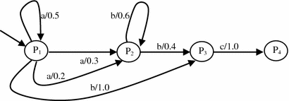

  

  Figure for Q3

[Hints: The sequences beginning at P₁ and terminating at P₄ are (Fig. 4.14):

Fig. 4.14

Hints for Q3

The probability of sequence bc = 1×1 = 1.0 is the highest.]

• 4. In the automaton provided in Fig. 4.15, suppose we have 4 patterns, to be introduced in the automaton for state transition. If today’s price falls in partition P₄, what would be the next appropriate time required for the state transition? Also what does prediction infer?

  Fig. 4.15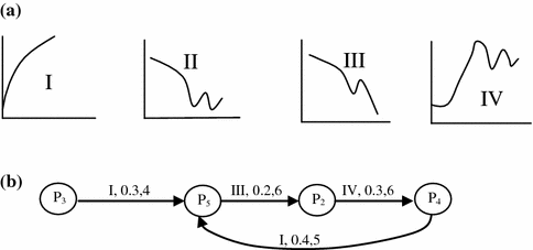

  

  a Clustered pattern used for prediction. b The automata representing transitions from one partition to the other with clustered patterns as input for state transition, the transition function includes input cluster, probability of transition and appropriate number of days required for transition in order

[Hints: Next state P₅, appropriate time required is 5 days. The prediction infers growth following cluster I.]

References

Barnea, O., Solow, A. R., & Stone, L. (2006). On fitting a model to a population time series with missing values. Israel Journal of Ecology and Evolution, 52, 1–10.
Chen, S. M., & Hwang, J. R. (2000). Temperature prediction using fuzzy time series. IEEE Transactions on Systems, Man, and Cybernetics, Part-B, 30(2), 263–275.
Wu, C. L., & Chau, K. W. (2013). Prediction of rainfall time series using modular soft computing methods. Elsevier, Engineering Applications of Artificial Intelligence, 26, 997–1007.
Jalil, A., & Idrees, M. (2013). Modeling the impact of education on the economic growth: Evidence from aggregated and disaggregated time series data of Pakistan. Elsevier Economic Modelling, 31, 383–388.
Song, Q., & Chissom, B. S. (1993). Fuzzy time series and its model. Elsevier, Fuzzy Sets Systems, 54(3), 269–277.
Song, Q., & Chissom, B. S. (1993). Forecasting enrollments with fuzzy time series—Part I. Elsevier, Fuzzy Sets Systems, 54(1), 1–9.
Mirikitani, D. T., & Nikolaev, N. (2010). Recursive Bayesian recurrent neural networks for time-series modeling. IEEE Transaction on Neural Networks, 2(2), 262–274.
Connor, J. T., Martin, R. D., & Atlas, L. E. (1994). Recurrent neural networks and robust time series prediction. IEEE Transaction on Neural Networks, 5(2), 240–254.
De Gooijer, J. G., & Hyndman, R. J. (2006). 25 years of time series forecasting. Elsevier, International Journal of Forecasting, 22, 443–473.
Lee, C. H. L., Liu, A., & Chen, W. S. (2006). Pattern discovery of fuzzy time series for financial prediction. IEEE Transactions on Knowledge and Data Engineering, 18(5), 613–625.
Bhattacharya, D., Konar, A., & Das, P. (2016). Secondary factor induced stock index time-series prediction using self-adaptive interval type-2 fuzzy sets. Elsevier, Neurocomputing, 171, 551–568.
Last, M., Klein, Y., & Kandel, A. (2001). Knowledge discovery in time series databases. IEEE Transactions on Systems, Man, and Cybernetics, Part B, 31(1), 160–169.
Dougherty, E. R., & Giardina, C. R. (1988). Mathematical methods for artificial intelligence and autonomous systems. USA: Prentice-Hall, The University of Michigan.
Ester, M., Kriegel, H. P., Sander, J., & Xu, X. (1996). A density-based algorithm for discovering clusters in large spatial databases with noise. In Proceedings of KDD-96 (pp. 226–231).
Konar, A. (1999). Artificial intelligence and soft computing: Behavioural and cognitive modeling of the human brain. Boca Raton, Florida: CRC Press.
TAIEX [Online]. Available http://www.twse.com.tw/en/products/indices/tsec/taiex.php
Bezdek, J. C., & Pal, N. R. (1998). Some new indexes of cluster validity. IEEE Transactions on Systems, Man, and Cybernetics, Part B, 28(3), 301–315.
Forgy, E. W. (1965). Cluster analysis of multivariate data: Efficiency versus interpretability of classification. Biometrics, 21(3), 768–769.
Bezdek, J. C. (1987). Pattern recognition with fuzzy objective function algorithms. New York and London: Plenum Press.
Edwards, R. D., Magee, J., & Bassetti, W. H. C. (2001). The dow theory. In Technical analysis of stock trends (8th ed., 2000, pp. 21–22). N.W. Corporate Blvd., Boca Raton, Florida: CRC Press LLC.
Keogh, E., Chu, S., Hart, D., & Pazzani, M. (2003). Segmenting time series: A survey and novel approach. Data mining in time series databases (2nd ed.). World Scientific.
Keogh, E., & Pazzani, M. (1999). Scaling up dynamic time warping to massive dataset. In Proceedings of third European conference principles of data mining and knowledge discovery (PKDD ’99) (pp. 1–11).
Kanth, K. V. R., Agrawal, D., & Singh, A. K. (1998). Dimensionality reduction for similarity searching in dynamic databases. In Proceedings of ACM SIGMOD ’98 (pp. 166–176).
Liu, X., Lin, Z., & Wang, H. (2008). Novel online methods for time series segmentation. IEEE Transactions of Knowledge and Data Engineering, 20(12), 1616–1626.
Appel, U., & Brandt, A. V. (1983). Adaptive sequential segmentation of piecewise stationary time series. Information Science, 29(1), 27–56.
Shatkay, H., & Zdonik, S. B. (1995). Approximate queries and representations for large data sequences. Technical report CS-95-03, Department of Computer Science, Brown University.
Keogh, E., & Smyth, P. (1997). A probabilistic approach to fast pattern matching in time series databases. In Proceedings of ACM SIGKDD’97 (pp. 20–24).
Bryant, G. F., & Duncan, S. R. (1994). A solution to the segmentation problem based on dynamic programming. In Proceedings of third IEEE conference of control applications (CCA ’94) (pp. 1391–1396).
Abonyi, J., Feil, B., Nemeth, S., & Arva, P. (2005). Modified Gath-Geva clustering for fuzzy segmentation of multivariate time-series. Elsevier, Fuzzy Sets and Systems, 149(1), 39–56.
Fuchs, E., Gruber, T., Nitschke, J., & Sick, B. (2010). Online segmentation of time series based on polynomial least-squares approximations. IEEE Transactions on Pattern Analysis, Machine Intelligence, 32(12), 2232–2245.
Chung, F. L., Fu, T. C., Ng, V., & Luk, R. W. P. (2004). An evolutionary approach to pattern-based time series segmentation. IEEE Transactions of Evolutionary Computation, 8(5), 471–489.
Xu, R., & Wunsch, D., II. (2005). Survey of clustering algorithms. IEEE Transactions on Neural Networks, 16(3), 645–678.
Mitchell, T. M. (1997). Machine learning. New York, USA: McGraw-Hill.
Liao, T. W. (2005). Clustering of time series data—a survey. Elsevier, Pattern Recognition, 38(11), 1857–1874.
Xiong, Z., Chen, R., Zhang, Y., & Zhang, X. (2012). Multi-density DBSCAN algorithm based on density levels partitioning. Journal of Information & Computational Science, 9(10), 2739–2749.
Lundberg, J. (2007). Lifting The Crown-Citation Z-score. Elsevier, Journal of Informatics, 1, 145–154.
http://computationalintelligence.net/tnnls/segmentation_performance.pdf
Author information
Authors and Affiliations
Corresponding author