
Abstract
In this chapter, we explain the fundamental principles of SAR data collection and image formation, i.e., inversion of the received data. Synthetic aperture radar uses microwaves for imaging the surface of the Earth from airplanes or satellites. Unlike photography which generates the picture by essentially recoding the intensity of the light reflected off the different parts of the target, SAR imaging exploits the phase information of the interrogating signals and as such can be categorized as a coherent imaging technology.
Access this chapter
Tax calculation will be finalised at checkout
Purchases are for personal use only
Notes
- 1.
In practice, u (1) is known at the receiving radar antenna, which is mounted on an airborne or spaceborne platform located above the imaged terrain (Earth’s surface), see Figure 2.1.
Fig. 2.1 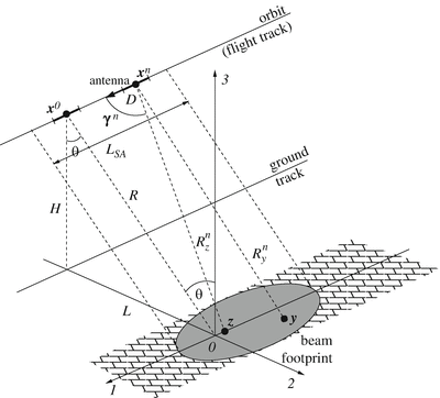
Schematic for the monostatic broadside stripmap SAR imaging. H is the orbit altitude, L is the distance (range) from the ground track to the target, R is the slant range, θ is the angle of incidence or the look angle, and D is the length of a linear antenna. (This figure is a modified version of [7, Figure 1]. Copyright ©2015 Society for Industrial and Applied Mathematics. Reprinted with permission. All rights reserved. Two different earlier versions have also appeared as [5, Figure 1] and [6, Figure 1]. Copyright ©2013, 2014 IOP Publishing. Reproduced with permission. All rights reserved.)
- 2.
In Section 2.6, we will see that a large value of Bτ is what enables the SAR resolution in range.
- 3.
We are assuming in (2.15’) that this distance is the same for both antennas, \(\boldsymbol{x}\) and \(\boldsymbol{x}^{{\prime}}\).
- 4.
- 5.
Grating lobes are responsible for the appearance of “ghost” images of bright targets shifted in azimuth with respect to their true location y 1 = z 1. Since the indicator function is only an approximation to the true antenna radiation pattern (see formulae (2.19) and (2.19’)), then in reality, the choice of the period X satisfying (2.49) will reduce the amplitude of grating lobes but not completely eliminate them.
- 6.
The role of the platform motion and the corresponding physical Doppler effect in SAR analysis is discussed in detail in Chapter 6
- 7.
- 8.
- 9.
The method of stationary phase provides only an approximate, rather than exact, value of the Fourier integral in (2.108). Therefore, the actual spectrum of the chirp (2.10), (2.11) extends beyond the interval ω ∈ [ω 0 − B∕2, ω 0 + B∕2]. Its more accurate computation would require the analysis of the case where the stationary point (2.110) is located at or near either of the endpoints of the integration interval t ∈ [−τ∕2, τ∕2], including the situation when it is outside of this interval, see, e.g., [112, Chapter III, Section 1] for detail. The exact spectrum of the chirp can be expressed via the erf( ⋅ ) functions of a complex argument, see, e.g., [5], although for obtaining practical estimates the resulting expressions still need to be approximated.

Bibliography
S.V. Tsynkov, On SAR imaging through the Earth’s ionosphere. SIAM J. Imaging Sci. 2 (1), 140–182 (2009)
E.M. Smith, S.V. Tsynkov, Dual carrier probing for spaceborne SAR imaging. SIAM J. Imaging Sci. 4 (2), 501–542 (2011)
M. Gilman, E. Smith, S. Tsynkov, Reduction of ionospheric distortions for spaceborne synthetic aperture radar with the help of image registration. Inverse Prob. 29 (5), 054005 (35 pp.) (2013)
M. Gilman, E. Smith, S. Tsynkov, Single-polarization SAR imaging in the presence of Faraday rotation. Inverse Prob. 30 (7), 075002 (27 pp.) (2014)
M. Gilman, S. Tsynkov, A mathematical model for SAR imaging beyond the first Born approximation. SIAM J. Imaging Sci. 8 (1), 186–225 (2015)
M. Cheney, B. Borden, Fundamentals of Radar Imaging. CBMS-NSF Regional Conference Series in Applied Mathematics, vol. 79 (SIAM, Philadelphia, 2009)
V.S. Ryaben’kii, S.V. Tsynkov, A Theoretical Introduction to Numerical Analysis (Chapman & Hall/CRC, Boca Raton, FL, 2007)
L.D. Landau, E.M. Lifshitz, Course of Theoretical Physics. Electrodynamics of Continuous Media, vol. 8 (Pergamon International Library of Science, Technology, Engineering and Social Studies. Pergamon Press, Oxford, 1984). Translated from the second Russian edition by J.B. Sykes, J.S. Bell, M.J. Kearsley, Second Russian edition revised by Lifshits and L.P. Pitaevskii
G. Franceschetti, R. Lanari, Synthetic Aperture Radar Processing. Electronic Engineering Systems Series (CRC Press, Boca Raton, FL, 1999)
L.J. Cutrona, Synthetic aperture radar, in Radar Handbook, 2nd edn., ed. by M. Skolnik, Chap. 21 (McGraw-Hill, New York, 1990)
I.G. Cumming, F.H. Wong, Digital Processing of Synthetic Aperture Radar Data. Algorithms and Implementation (Artech House, Boston, 2005)
M. Cheney, A mathematical tutorial on synthetic aperture radar. SIAM Rev. 4 3(2), 301–312 (electronic) (2001)
L.D. Landau, E.M. Lifshitz, Course of Theoretical Physics. The Classical Theory of Fields, vol. 2, 4th edn. (Pergamon Press, Oxford, 1975). Translated from the Russian by Morton Hamermesh
M. Born, E. Wolf, Principles of Optics: Electromagnetic Theory of Propagation, Interference and Diffraction of Light. With contributions by A.B. Bhatia, P.C. Clemmow, D. Gabor, A.R. Stokes, A.M. Taylor, P.A. Wayman, W.L. Wilcock, seventh (expanded) edition (Cambridge University Press, Cambridge, 1999)
A. Papoulis, Signal Analysis (McGraw-Hill, New York, 1977)
H.A. Zebker, J. Villasenor, Decorrelation in interferometric radar echoes. IEEE Trans. Geosci. Remote Sens. 30 (5), 950–959 (1992)
M.V. Fedoryuk, The Saddle-Point Method [Metod perevala] (Nauka, Moscow, 1977) [Russian]
Author information
Authors and Affiliations
Appendix 2.A Choosing the matched filter
Appendix 2.A Choosing the matched filter
Let the received field be given by the integral [cf. formula (2.14”)]
where \(\nu (\boldsymbol{z})\) incorporates both the ground reflectivity and the propagation attenuation, see (2.15’), and let the image be defined with the help of the function \(K = K(t,\boldsymbol{y})\) [cf. formula (2.24)]:
Substituting (2.98) into (2.99) and changing the order of integration, we arrive at a mapping \(\nu (\boldsymbol{z})\mapsto I_{\boldsymbol{x}}(\boldsymbol{y})\), which is known as the imaging operator:
The function \(K(t,\boldsymbol{y})\), which is at our disposal, can be chosen to achieve some desirable properties of the imaging operator (2.100).
One of those properties may be to maximize the return from isolated point scatterers. Namely, let \(\nu (\boldsymbol{z}) =\nu _{\boldsymbol{z}_{0}}\delta (\boldsymbol{z} -\boldsymbol{z}_{0})\), where \(\nu _{\boldsymbol{z}_{0}}\) is a constant factor and \(\boldsymbol{z}_{0}\) is given. Then, formula (2.100) yields:
Assume that the function \(K(t,\boldsymbol{y})\) is absolutely square integrable with respect to t uniformly in \(\boldsymbol{y}\), i.e., \(\forall \boldsymbol{y}:\ K(t,\boldsymbol{y}) \in L_{2}(-\infty,\infty )\), and the estimate
holds with one and the same constant E K for all \(\boldsymbol{y}\). Consider the image (2.101) at \(\boldsymbol{y} = \boldsymbol{z}_{0}\). We will seek \(K(t,\boldsymbol{y})\) that maximizes the return \(I_{\boldsymbol{x}}(\boldsymbol{z}_{0})\) relative to the input \(\nu _{\boldsymbol{z}_{0}}\), i.e., maximizes the ratio \(\frac{\vert I_{\boldsymbol{x}}(\boldsymbol{z}_{0})\vert } {\vert \nu _{\boldsymbol{z}_{0}}\vert }\), subject to constraint (2.102).
From the Cauchy-Schwarz inequality we get the following estimate:
where
For the chirp (2.10), (2.11), E P = τ. The equality in (2.103) is reached only for
Formula (2.104) defines the matched filter: the kernel in the integral operator (2.99) is a scaled delayed complex conjugate replica of the original signal. Moreover, it is easy to see that the resulting maximum value of \(\frac{\vert I_{\boldsymbol{x}}(\boldsymbol{z}_{0})\vert } {\vert \nu _{\boldsymbol{z}_{0}}\vert }\) appears independent of \(\boldsymbol{z}_{0}\). If we take E K = τ, then formula (2.104) reduces to the expression (2.23) for the matched filter that we introduced in Section 2.3.1.
The consideration based solely on point scatterers is deficient though in that the real radar targets may have a different composition. As such, instead of maximizing the return from point scatterers we may require that the kernel of the imaging operator (2.100), i.e., the PSF
be close to the delta-function \(\delta (\boldsymbol{y} -\boldsymbol{ z})\). This requirement is more general than the previous one because in the case of a true equality: \(W_{\boldsymbol{x}}(\boldsymbol{y},\boldsymbol{z}) =\delta (\boldsymbol{y} -\boldsymbol{ z})\), the image \(I(\boldsymbol{y})\) on the left-hand side of (2.100) exactly reconstructs the unknown function \(\nu (\boldsymbol{z})\) regardless of its actual form.
Yet the question of how one shall understand the “closeness” between \(W_{\boldsymbol{x}}(\boldsymbol{y},z)\) and \(\delta (\boldsymbol{y} -\boldsymbol{ z})\) requires attention, because spaces of distributions are not equipped with norms. We will use the spectral interpretation, i.e., employ the Fourier transform. Namely, let \(\tilde{K}\) and \(\tilde{P}\) denote the Fourier transforms of K and P, respectively, in time:
Then, taking into account that the Fourier transform of a product is the convolution of Fourier transforms, for the PSF (2.105) we can write:
For the rest of this section, we will adopt a simplified one-dimensional setting, for which \(\boldsymbol{y} = R_{\boldsymbol{y}} \equiv y\) and \(\boldsymbol{z} = R_{\boldsymbol{z}} \equiv z\). Then, the following identity holds:
Matching the right-hand side of the previous equality against that of (2.106), we see that if
then the spectra of the two expressions differ only by the constant \(\frac{2} {c}\), which is not essential. Consequently, if (2.107) could be satisfied for all ω, then \(W_{\boldsymbol{x}}(y,z)\) will be proportional to δ(y − z), which is our goal.
However, choosing \(\tilde{K}(\omega,y)\) to satisfy (2.107) for all \(\omega \in \mathbb{R}\) is not possible if \(\tilde{P}(\omega )\) is zero (or very small by absolute value) for a range of frequencies. This appears to be the case for the chirped signals (2.10), (2.11) that are designed to have their spectrum confined to a band of width B around the central carrier frequency ω 0:
The integration in (2.108) has been performed using the method of stationary phase, and the factor
on the last line of (2.108) originates from the condition that the stationary point of the phase
must belong to the interval [−τ∕2, τ∕2] defined by the indicator function χ τ (t) of (2.11).Footnote 9 It is only in the frequency band \(\vert \omega -\omega _{0}\vert \leqslant B/2\) defined by (2.109) that \(\tilde{K}(\omega,y)\) can be chosen to satisfy (2.107):
where \(\tilde{\overline{P}}(\omega )\) denotes the Fourier transform of the complex conjugate of P(t), and the second equality in (2.111) is derived with the help of (2.108) and (2.109). Applying the inverse Fourier transform to (2.111), we obtain:
which coincides with the matched filter expression (2.104). Hence, for the chirped signals the matched filter formula (2.104) also satisfies (2.107) so that the spectrum of \(W_{\boldsymbol{x}}(y,z) = W_{\boldsymbol{x}}(y - z)\) coincides with that of δ(y − z) for \(\vert \omega -\omega _{0}\vert \leqslant B/2\). In this sense, \(W_{\boldsymbol{x}}(y - z)\) can be considered an approximation to δ(y − z).
Rights and permissions
Copyright information
© 2017 Springer International Publishing AG
About this chapter
Cite this chapter
Gilman, M., Smith, E., Tsynkov, S. (2017). Conventional SAR imaging. In: Transionospheric Synthetic Aperture Imaging. Applied and Numerical Harmonic Analysis. Birkhäuser, Cham. https://doi.org/10.1007/978-3-319-52127-5_2
Download citation
DOI: https://doi.org/10.1007/978-3-319-52127-5_2
Published:
Publisher Name: Birkhäuser, Cham
Print ISBN: 978-3-319-52125-1
Online ISBN: 978-3-319-52127-5
eBook Packages: Mathematics and StatisticsMathematics and Statistics (R0)