
Abstract
In this chapter, self-dual and binary double-circulant codes based on primes are discussed. Many double-circulant codes are self-dual. Binary self-dual codes form an important class of codes due to their powerful error-correcting capabilities and their rich mathematical structure. This structure enables the entire weight distribution of a code to be determined. With these interesting properties, this family of codes has been a subject of extensive research for many years. For these codes that are longer than around 150 bits, an accurate determination of the codeword weight distributions has been an unsolved challenge. We show that the code structure may be used in a new algorithm that requires less codewords to be enumerated than traditional methods. We describe the new algorithm in detail and present new, complete, weight distribution results for codes of length 152, 168, 192, 194 and 200. We describe a modular congruence method and show how it can be used to check weight distributions of codes and have corrected some mistakes in previously published results for codes of length 137 and 151. For evaluation of the minimum Hamming distance for very long codes, a new probabilistic method has been presented along with results for codes up to 450 bits long. It is conjectured that the (136, 68, 24) self-dual code is the longest extremal code, meeting the upper bound for minimum Hamming distance, and that no other, longer, extremal code exists.
You have full access to this open access chapter, Download chapter PDF
1 Introduction
Binary self-dual codes have an interesting structure and some are known to have the best possible minimum Hamming distance of any known codes. Closely related to the self-dual codes are the double-circulant codes. Many good binary self-dual codes can be constructed in double-circulant form. Double-circulant codes as a class of codes have been the subject of a great deal of attention, probably because they include codes, or the equivalent codes, of some of the most powerful and efficient codes known to date. An interesting family of binary, double-circulant codes, which includes self-dual and formally self-dual codes, is the family of codes based on primes. A classic paper for this family was published by Karlin [9] in which double-circulant codes based on primes congruent to \(\pm 1\) and \(\pm 3\) modulo 8 were considered. Self-dual codes are an important category of codes because there are bounds on their minimal distance [1]. The possibilities for their weight spectrum are constrained, and known ahead of the discovery, and analysis of the codes themselves. This has created a great deal of excitement among researchers in the rush to be the first in finding some of these codes. A paper summarising the state of knowledge of these codes was given by Dougherty et al. [1]. Advances in high-speed digital processors now make it feasible to implement near maximum likelihood, soft decision decoders for these codes and thus, make it possible to approach the predictions for frame error rate (FER) performance for the additive white Gaussian noise channel made by Claude Shannon back in 1959 [16].
This chapter considers the binary double-circulant codes based on primes, especially in analysis of their Hamming weight distributions. Section 9.2 introduces the notation used to describe double-circulant codes and gives a review of double-circulant codes based on primes congruent to \(\pm 1\) and \(\pm 3\) modulo 8. Section 9.4 describes the construction of double-circulant codes for these primes and Sect. 9.5 presents an improved algorithm to compute the minimum Hamming distance and also the number of codewords of a given Hamming weight for certain double-circulant codes. The algorithm presented in this section requires the enumeration of less codewords than that of the commonly used technique [4, 18] e.g. Sect. 9.6 considers the Hamming weight distribution of the double-circulant codes based on primes. A method to provide an independent verification to the number of codewords of a given Hamming weight in these double-circulant codes is also discussed in this section. In the last section of this chapter, Sect. 9.7, a probabilistic method−based on its automorphism group, to determine the minimum Hamming distance of these double-circulant codes is described.
Note that, as we consider Hamming space only in this chapter, we shall omit the word “Hamming” when we refer to Hamming weight and distance.
2 Background and Notation
A code \(\mathscr {C}\) is called self-dual if,
where \(\mathscr {C}^\perp \) is the dual of \(\mathscr {C}\) . There are two types of self-dual code: doubly even or Type-II for which the weight of every codeword is divisible by 4; singly even or Type-I for which the weight of every codeword is divisible by 2. Furthermore, the code length of a Type-II code is divisible by 8. On the other hand, formally self-dual (FSD) codes are codes that have
but satisfy \(A_{\mathscr {C}}(z) = A_{\mathscr {C}^\perp }(z)\), where \(A(\mathscr {C})\) denotes the weight distribution of the code \(\mathscr {C}\). A self-dual, or FSD, code is called extremal if its minimum distance is the highest possible given its parameters. The bound of the minimum distance of the extremal codes is [15]
where
for an extremal FSD code with length n and minimum distance d. For an FSD code, the minimum distance of the extremal case is upper bounded by [4]
As a consequence of this upper bound, extremal FSD codes are known to only exist for lengths \(n \le 30\) and \(n \not = 16\) and \(n \not = 26\) [7]. Databases of best-known, not necessary extremal, self-dual codes are given in [3, 15]. A table of binary self-dual double-circulant codes is also provided in [15].
As a class, double-circulant codes are (n, k) linear codes, where \(k=n/2\), whose generator matrix \(\varvec{G}\) consists of two circulant matrices.
Definition 9.1
( Circulant Matrix) A circulant matrix is a square matrix in which each row is a cyclic shift of the adjacent row. In addition, each column is also a cyclic shift of the adjacent column and the number of non-zeros per column is equal to those per row.
A circulant matrix is completely characterised by a polynomial formed by its first row
which is called the defining polynomial.
Note that the algebra of polynomials modulo \(x^m-1\) is isomorphic to that of circulants [13]. Let the polynomial r(x) have a maximum degree of m, and the corresponding circulant matrix \(\varvec{R}\) is an \(m \times m\) square matrix of the form
where the polynomial in each row can be represented by an m-dimensional vector, which contains the coefficients of the corresponding polynomial.
2.1 Description of Double-Circulant Codes
A double-circulant binary code is an \((n,\frac{n}{2})\) code in which the generator matrix is defined by two circulant matrices, each matrix being \(\frac{n}{2}\) by \(\frac{n}{2}\) bits. Circulant consists of cyclically shifted rows, modulo \(\frac{n}{2}\), of a generator polynomial. These generator polynomials are defined as \(r_1(x)\) and \(r_2(x)\). Each codeword consists of two parts: the information data, defined as u(x), convolved with \(r_1(x)\) modulo (\(1+x^\frac{n}{2}\)) adjoined with u(x) and convolved with \(r_2(x)\) modulo (\(1+x^\frac{n}{2}\)). The code is the same as a non-systematic, tail-biting convolutional code of rate one half. Each codeword is \([u(x)r_1(x),u(x)r_2(x)]\). If \(r_1(x)\) [or \(r_2(x)\)] has no common factors of (\(1+x^\frac{n}{2}\)), then the respective circulant matrix is non-singular and may be inverted. The inverted circulant matrix becomes an identity matrix, and each codeword is defined by u(x), u(x)r(x), where \(r(x)=\frac{r_1(x)}{r_2(x)}\text { modulo } (1+x^\frac{n}{2})\), [or \(r(x)=\frac{r_2(x)}{r_1(x)}\text { modulo }(1+x^\frac{n}{2})\), respectively]. The code is now the same as a systematic, tail-biting convolutional code of rate one half.
For double-circulant codes where one circulant matrix is non-singular and may be inverted, the codes can be put into two classes, namely pure, and bordered double-circulant codes, whose generator matrices \(\varvec{G}_p\) and \(\varvec{G}_b\) are shown in (9.5a)

and (9.5b),

respectively. Here, \(\varvec{I}_k\) is a k-dimensional identity matrix, and \(\alpha \in \{0,1\}\).
Definition 9.2
( Quadratic Residues) Let \(\alpha \) be a generator of the finite field \(\mathbb {F}_p\), where p be an odd prime, \(r \equiv \alpha ^2 \pmod p\) is called a quadratic residue modulo p and so is \(r^{i}\in \mathbb {F}_p\) for some integer i. Because the element \(\alpha \) has (multiplicative) order \(p-1\) over \(\mathbb {F}_p\), \(r = \alpha ^2\) has order \(\frac{1}{2}(p-1)\). A set of quadratic residues modulo p, Q and non-quadratic residues modulo p, N, are defined as
and
respectively.
As such \(R\cup Q \cup \{0\}=\mathbb {F}_p\). It can be seen from the definition of Q and N that, if \(r \in Q\), \(r = \alpha ^e\) for even e; and if \(n \in N\), \(n = \alpha ^e\) for odd e. Hence, if \(n\in N\) and \(r\in Q\), \(rn = \alpha ^{2i}\alpha ^{2j+1} = \alpha ^{2(i+j)+1}\in N\). Similarly, \(rr =\alpha ^{2i}\alpha ^{2j} = \alpha ^{2(i+j)} \in Q\) and \(nn = \alpha ^{2i + 1}\alpha ^{2j + 1} = \alpha ^{2(i+j+1)} \in Q\).
Furthermore,
-
\(2\in Q\) if \(p\equiv \pm 1 \pmod { 8}\), and \(2\in N\) if \(p\equiv \pm 3 \pmod { 8}\)
-
\(-1\in Q\) if \(p\equiv 1 \pmod { 8}\) or \(p\equiv -3 \pmod { 8}\), and \(-1\in N\) if \(p\equiv -1 \pmod { 8}\) and \(p\equiv 3 \pmod { 8}\)
3 Good Double-Circulant Codes
3.1 Circulants Based Upon Prime Numbers Congruent to \({\pm }\)3 Modulo 8
An important category is circulants whose length is equal to a prime number, p, which is congruent to \(\pm 3\) modulo 8. For many of these prime numbers, there is only a single cyclotomic coset, apart from zero. In these cases, \(1+x^p\) factorises into the product of two irreducible polynomials, \((1+x)(1+x+x^2+x^3+\cdots +x^{p-1})\). Apart from the polynomial, \((1+x+x^2+x^3+\cdots +x^{p-1})\), all of the other \(2^p-2\) non-zero polynomials of degree less than p are in one of two sets: The set of \(2^{p-1}\) even weight, polynomials with \(1+x\) as a factor, denoted as \(\mathbf {S_f}\), and the set of \(2^{p-1}\) odd weight polynomials which are relatively prime to \(1+x^p\), denoted as \(\mathbf {S_r}\). The multiplicative order of each set is \(2^{p-1}-1\), and each forms a ring of polynomials modulo \(1+x^p\). Any non-zero polynomial apart from \((1+x+x^2+x^3+\cdots +x^{p-1})\) is equal to \(\alpha (x)^i\) for some integer i if the polynomial is in \(\mathbf {S_f}\) or is equal to \(a(x)^i\) for some integer i if in \(\mathbf {S_r}\). An example for \(p=11\) is given in Appendix “Circulant Analysis \(p=11\)”. In this table, \(\alpha (x)=1+x+x^2+x^4\) and \(a(x)=1+x+x^3\). For these primes, as the circulant length is equal to p, the generator polynomial r(x) can either contain \(1+x\) as a factor, or not contain \(1+x\) as a factor, or be equal to \((1+x+x^2+x^3+\cdots +x^{p-1})\). For the last case, this is not a good choice for r(x) as the minimum codeword weight is 2, which occurs when \(u(x)=1+x\). In this case, \(r(x)u(x)=1+x^p=0 \text { modulo } 1+x^p\) and the codeword is \([1+x,\,0]\), a weight of 2.
When r(x) is in the ring \(\mathbf {S_f}\), u(x)r(x) must also be in \(\mathbf {S_f}\) and therefore, be of even weight, except when \(u(x)=(1+x+x^2+x^3+\cdots +x^{p-1})\).
In this case \(u(x)r(x)=0 \text { modulo } 1+x^p\) and the codeword is \([1+x+x^2+x^3+\cdots +x^{p-1}, 0]\) of weight p. When u(x) has even weight, the resulting codewords are doubly even. When u(x) has odd weight, the resulting codewords consist of two parts, one with odd weight and the other with even weight. The net result is the codewords that always have odd weight. Thus, there are both even and odd weight codewords when u(x) is from \(\mathbf {S_f}\).
When r(x) is in the ring \(\mathbf {S_r}\), u(x)r(x) is always non-zero and is in \(\mathbf {S_f}\) (even weight) only when u(x) has even weight, and the resulting codewords are doubly even. When u(x) has odd weight, \(u(x)=a(x)^j\) and \(u(x)r(x)=a(x)^ja(x)^i=a(x)^{i+j}\) and hence is in the ring \(\mathbf {S_f}\) and has odd weight. The resulting codewords have even weight since they consist of two parts, each with odd weight. Thus, when r(x) is from \(\mathbf {S_r}\) all of the codewords have even weight. Furthermore, since \(r(x)=a(x)^i\), \(r(x)a(x)^{2^{(p-1)}-1-i}=a(x)^{2^{(p-1)}-1}=1\) and hence, the inverse of r(x), \(\frac{1}{g(x)}=a(x)^{2^{(p-1)}-1-i}\).
By constructing a table (or sampled table) of \(\mathbf {S_r}\), it is very straightforward to design non-singular double-circulant codes. The minimum codeword weight of the code \(d_{min}\) cannot exceed the weight of \(r(x)+1\). Hence, the weight of \(a(x)^i\) needs to be at least \(d_{min}-1\) to be considered as a candidate for r(x). The weight of the inverse of r(x), \(a(x)^{2^{(p-1)}-1-i}\) also needs to be at least \(d_{min}-1\). For odd weight \(u(x)=a(x)^j\) and \(u(x)r(x)=a(x)^j a(x)^i=a(x)^{(j+i)}\). Hence, the weight of u(x)r(x) can be found simply by looking up the weight of \(a(x)^{i+j}\) from the table. Self-dual codes are those with \(\frac{1}{r(x)}=r(x^{-1})\). With a single cyclotomic coset \(2^\frac{(p-1)}{2}=-1\), and it follows that \(a(x)^{2^\frac{(p-1)}{2}}=a(x^{-1})\). With \(r(x)=a(x)^i\), \(r(x^{-1})=a(x)^{{2^\frac{(p-1)}{2}}i}\).
In order that \( \frac{1}{r(x)}=r(x^{-1})\), it is necessary that
Equating the exponents, modulo \(2^{(p-1)}-1\), gives
where m is an integer. Solving for i:
Hence, the number of distinct self-dual codes is equal to \((2^\frac{(p-1)}{2}+1)\).
For the example, \(p=13\) as above,
and there are \(2^\frac{(p-1)}{2}+1=65\) self-dual codes for \(1 \le j \le 65\) and these are \(a(x)^{63}\), \(a(x)^{126}\), \(a(x)^{189},\ldots , a(x)^{4095}\).
As p is congruent to \(\pm 3\), the set \((u(x)r(x))^{2^t}\) maps to (u(x)r(x)) for \(t=1\,\rightarrow r\), where r is the size of the cyclotomic cosets of \(2^\frac{(p-1)}{2}+1\). In the case of \(p=13\) above, there are 4 cyclotomic cosets of 65, three of length 10 and one of length 2. This implies that there on 4 non-equivalent self-dual codes.
For p congruent to \(-3\) modulo 8, \((2^\frac{(p-1)}{2}+1)\) is not divisible by 3. This means that the pure double-circulant quadratic residue code is not self-dual. Since the quadratic residue code has multiplicative order 3, this means that for p congruent to \(-3\) modulo 8, the quadratic residue, pure double-circulant code is self-orthogonal, and \(r(x)=r(x^{-1})\).
For p congruent to 3, \((2^\frac{(p-1)}{2}+1)\) is divisible by 3 and the pure double-circulant quadratic residue code is self-dual. In this case, a(x) has multiplicative order of \(2^{(p-1)}-1\), and \(a(x)^{\frac{(2^{(p-1)}-1)}{3}}\) must have exponents equal to the quadratic residues (or non-residues). The inverse polynomial is \(a(x)^{\frac{2(2^{(p-1)}-1)}{3}}\) with exponents equal to the non-residues (or residues, respectively), and defines a self-dual circulant code. As an example, for \(p=11\) as listed in Appendix “Circulant Analysis \(p=11\)”, \(2^{(p-1)}-1=1023\) and \(a(x)^{341} = x+x^3 +x^4 +x^5+x^9 \), the quadratic non-residues of 11 are 1, 4, 5, 9 and 3. \(a(x)^{682}= x^2+x^6 +x^7 +x^8+x^{10} \) corresponding to the quadratic residues: 2, 8, 10, 7 and 6 as can be seen from Appendix “Circulant Analysis \(p=11\)”. Section 9.4.3 discusses in more detail pure double-circulant codes for these primes.
3.2 Circulants Based Upon Prime Numbers Congruent to ±1 Modulo 8: Cyclic Codes
MacWilliams and Sloane [13] discuss the Automorphism group of the extended cyclic quadratic residue (eQR) codes and show that this includes the projective special linear group \(PSL_2(p)\) . They describe a procedure in which a double-circulant code may be constructed from a codeword of the eQR code. It is fairly straightforward. The projective special linear group \(PSL_2(p)\) for a prime p is defined by the permutation \(y\rightarrow \frac{ay+b}{cy+d}\) mod p, where the integers a, b, c, d are such that two cyclic groups of order \(\frac{p+1}{2}\) are obtained. A codeword of the \((p+1,\frac{p+1}{2})\) eQR code is obtained and the non-zero coordinates of the codeword placed in each cyclic group. This splits the codeword into two cyclic parts each of which defines a circulant polynomial.
The procedure is best illustrated with an example. Let \(\alpha \in \mathbb {F}_{p^2}\) be a primitive \((p^2-1)^{\text {ti}}\) root of unity; then, \(\beta =\alpha ^{2p-2}\) is a primitive \(\frac{1}{2}(p+1)^{\text {TA}}\) root of unity since \(p^2-1=\frac{1}{2}(2p-2)(p-1)\). Let \(\lambda =1/(1+\beta )\) and \(a=\lambda ^2-\lambda \); then, the permutation \(\pi _1\) on a coordinate y is defined as
where \(\pi _1 \in \text {PSL}_2(p)\) (see Sect. 9.4.3 for the definition of \(\text {PSL}_2(p))\). As an example, consider the prime \(p=23\). The permutation \(\pi _1: y\rightarrow \frac{y+1}{5y}\) mod p produces the two cyclic groups
and
There are 3 cyclotomic cosets for \(p=23\) as follows:
The idempotent given by \(C_1\) may be used to define a generator polynomial, r(x), which defines the (23, 12, 7) cyclic quadratic residue code:
Codewords of the (23, 12, 7) cyclic code are given by u(x)r(x) modulo \(1+x^{23}\) and with \(u(x)=1\) the non-zero coordinates of the codeword obtained are
the cyclotomic coset \(C_1\).
The extended code has an additional parity check using coordinate 23 to produce the corresponding codeword of the extended (24, 12, 8) code with the non-zero coordinates:
Mapping these coordinates to the cyclic groups with 1 in the position, where each coordinate is in the respective cyclic group and 0 otherwise, produces
and
which define the two circulant polynomials, \(r_1(x)\) and \(r_2(x)\), for the (24, 12, 8) pure double-circulant code
The inverse of \(r_1(x)\;\text {modulo }(1+x^{12})\) is \(\psi (x)\), where
and this may be used to produce an equivalent (24, 12, 8) pure double-circulant code which has the identity matrix as the first circulant
After evaluating terms, the two circulant polynomials are found to be
and it can be seen that the first circulant will produce the identity matrix of dimension 12. Jenson [8] lists the circulant codes for primes \(p<200\) that can be constructed in this way. There are two cases, \(p=89\) and \(p=167\), where a systematic double-circulant construction is not possible. A non-systematic double-circulant code is possible for all cases but the existence of a systematic code depends upon one of the circulant matrices being non-singular. Apart from \(p=89\) and \(p=167\) (for \(p < 200\)) a systematic circulant code can always be constructed in each case.
Table 9.1 lists the best circulant codes as a function of length. Most of these codes are well known and have been previously published but not necessarily as circulant codes. Moreover, the \(d_{min}\) of some of the longer codes have only been bounded and have not been explicitly stated in the literature. Nearly, all of the best codes are codes based upon the two types of quadratic residue circulant codes. For codes based upon \(p= \pm 3\quad mod \, 8\), it is an open question whether a better circulant code exists than that given by the quadratic residues. For \(p= \pm 1\quad mod\, 8\), there are counter examples. For example, the (72, 36, 14) code in Table 9.1 is better than the (72, 36, 12) circulant code which is based upon the extended cyclic quadratic residue code of length 71. The circulant generator polynomial g(x) for all of the codes of Table 9.1 is given in Table 9.2.
In Table 9.1, where the best (2p, p) code is given as b(x), the \((2p+2,p+1)\) circulant code can still be constructed from \(\beta (x)\) but this code has the same \(d_{min}\) as the pure, double-circulant, shorter code. For example, for the prime 109, b(x) produces a double-circulant (218, 109, 30) code. The polynomial \(\beta (x)\) produces a double-circulant (218, 109, 29) code, which bordered becomes a (220, 110, 30) code. It should be noted that \(\beta (x)\) need not have the overall parity bit border added. In this case, a \((2p+1,p+1)\) code is produced but with the same \(d_{min}\) as the \(\beta (x)\) code. In the latter example, a (219, 110, 29) code is produced.
4 Code Construction
Two binary linear codes, \(\mathscr {A}\) and \(\mathscr {B}\), are equivalent if there exists a permutation \(\pi \) on the coordinates of the codewords which maps the codewords of \(\mathscr {A}\) onto codewords of \(\mathscr {B}\). We shall write this as \(\mathscr {B} = \pi (\mathscr {A})\). If \(\pi \) transforms \(\mathscr {C}\) into itself, then we say that \(\pi \) fixes the code, and the set of all permutations of this kind forms the automorphism group of \(\mathscr {C}\), denoted as \(\text {Aut}(\mathscr {C})\). MacWilliams and Sloane [13] gives some necessary but not sufficient conditions on the equivalence of double-circulant codes, which are restated for convenience in the lemma below.
Lemma 9.1
(cf. [13, Problem 7, Chap. 16]) Let \(\mathscr {A}\) and \(\mathscr {B}\) be double-circulant codes with generator matrices \([\varvec{I}_k|\varvec{A}]\) and \([\varvec{I}_k|\varvec{B}]\), respectively. Let the polynomials a(x) and b(x) be the defining polynomials of \(\varvec{A}\) and \(\varvec{B}\). The codes \(\mathscr {A}\) and \(\mathscr {B}\) are equivalent if any of the following conditions holds:
-
(i)
\(\varvec{B}=\varvec{A}^T\), or
-
(ii)
b(x) is the reciprocal of a(x), or
-
(iii)
\(a(x)b(x)=1 \pmod { x^m-1}\), or
-
(iv)
\(b(x)=a(x^u)\), where m and u are relatively prime.
Proof
-
(i)
We can clearly see that \(b(x) = \sum _{i=0}^{m-1}a_ix^{m-i}\). It follows that \(b(x) = \pi (a(x))\), where \(\pi : i \rightarrow m-i\text { (mod }m)\) and hence, \(\mathscr {A}\) and \(\mathscr {B}\) are equivalent.
-
(ii)
Given a polynomial a(x), its reciprocal polynomial can be written as \(\bar{a}(x) = \sum _{i=0}^{m-1} a_i x^{m-i-1}\). It follows that \(\bar{a}(x) = \pi (a(x))\), where \(\pi : i \rightarrow m-i-1\text { (mod }m)\).
-
(iii)
Consider the code \(\mathscr {A}\), since b(x) has degree less than m, it can be one of the possible data patterns and in this case, the codeword of \(\mathscr {A}\) has the form |b(x) |1|. Clearly, this is a permuted codeword of \(\mathscr {B}\).
-
(iv)
If \((u,m) = 1\), then \(\pi : i \rightarrow iu \text { (mod }m)\) is a permutation on \(\{0,1,\ldots ,m-1\}\). So \(b(x) = a(x^u)\) is in the code \(\pi (\mathscr {A})\).
Consider an (n, k, d) pure double-circulant code, we can see that for a given user message, represented by a polynomial u(x) of degree at most \(k-1\), a codeword of the double-circulant code has the form \(\left( u(x) | u(x)r(x) \pmod { x^m-1}\right) \). The defining polynomial r(x) characterises the resulting double-circulant code. Before the choice of r(x) is discussed, consider the following lemmas and corollary.
Lemma 9.2
Let a(x) be a polynomial over \(\mathbb {F}_2\) of degree at most \(m-1\), i.e. \(a(x) = \sum _{i=0}^{m-1} a_i x^i\) where \(a_i\in \{0,1\}\). The weight of the polynomial \((1+x)a(x) \pmod { x^m-1}\), denoted by \(\mathrm {wt}_H((1+x)a(x))\) is even.
Proof
Let \(w = \mathrm {wt}_H(a(x)) = \mathrm {wt}_H(xa(x))\) and \(S=\{ i : a_{i+1\text { mod }m} = a_i \ne 0,~0 \le i \le m-1 \}\):
which is even.
Lemma 9.3
An \(m \times m\) circulant matrix \(\varvec{R}\) with defining polynomial r(x) is non-singular if and only if r(x) is relatively prime to \(x^m - 1\).
Proof
If r(x) is not relatively prime to \(x^m-1\), i.e. GCD \((r(x), x^m-1) = t(x)\) for some polynomial \(t(x) \ne 1\), then from the extended Euclidean algorithm, it follows that, for some unique polynomials a(x) and b(x), \(r(x)a(x) + (x^m-1)b(x) = 0\), and therefore \(\varvec{R}\) is singular.
If r(x) is relatively prime to \(x^m-1\), i.e. GCD \((r(x), x^m-1) = 1\), then from the extended Euclidean algorithm, it follows that, for some unique polynomials a(x) and b(x), \(r(x)a(x) + (x^m-1)b(x) = 1\), which is equivalent to \(r(x)a(x) = 1 \pmod { x^m-1}\). Hence \(\varvec{R}\) is non-singular, being invertible with a matrix inverse whose defining polynomial is a(x).
Corollary 9.1
From Lemma 9.3,
-
(i)
if \(\varvec{R}\) is non-singular, \(\varvec{R}^{-1}\) is an \(m \times m\) circulant matrix with defining polynomial \(r(x)^{-1}\), and
-
(ii)
the weight of r(x) or \(r(x)^{-1}\) is odd.
Proof
The proof for the first case is obvious from the proof of Lemma 9.3. For the second case, if the weight of r(x) is even then r(x) is divisible by \(1+x\). Since \(1+x\) is a factor of \(x^m-1\) then r(x) is not relatively prime to \(x^m-1\) and the weight of r(x) is necessarily odd. The inverse of \(r(x)^{-1}\) is r(x) and for this to exist \(r(x)^{-1}\) must be relatively prime to \(x^m-1\) and the weight of \(r(x)^{-1}\) is necessarily odd.
Lemma 9.4
Let p be an odd prime, and then
-
(i)
\(p \mid 2^{p-1} - 1\), and
-
(ii)
the integer q for \(pq = 2^{p-1} - 1\) is odd.
Proof
From Fermat’s little theorem, we know that for any integer a and a prime p, \(a^{p-1} \equiv 1 \pmod p\). This is equivalent to \(a^{p-1} - 1 = pq\) for some integer q. Let \(a = 2\), we have
which is clearly odd since neither denominator nor numerator contains 2 as a factor.
Lemma 9.5
Let p be a prime and \(j(x) = \sum _{i=0}^{p-1} x^i\); then
Proof
We can write \((1+x)^{2^{p-1}-1}\) as
From Lemma 9.4, we know that the integer \(q = (2^{p-1} - 1)/p\) and is odd. We can then write \(\sum _{i=0}^{2^{p-1}-1} x^i\) in terms of j(x) as follows:
Since \((1+x^p) \pmod { x^p-1} = 0\) for a binary polynomial, \(J(x)=0\) and we have
Because \(x^{ip} \pmod { x^p-1} = 1\),
For the rest of this chapter, we consider the bordered case only and for convenience, unless otherwise stated, we shall assume that the term double-circulant code refers to (9.5b). Furthermore, we call the double-circulant codes based on primes congruent to \(\pm 1\) modulo 8, the \([p+1, \frac{1}{2}(p+1), d]\) extended quadratic residue (QR) codes since these exist only for \(p\equiv \pm 1 \pmod 8\).
Following Gaborone [2], we call those double-circulant codes based on primes congruent to \(\pm 3\) modulo 8 the \([2(p+1), p+1, d]\) quadratic double-circulant (QDC) codes, i.e. \(p\equiv \pm 3 \pmod 8\).
4.1 Double-Circulant Codes from Extended Quadratic Residue Codes
The following is a summary of the extended QR codes as double-circulant codes [8, 9, 13].
Binary QR codes are cyclic codes of length p over \(\mathbb {F}_2\). For a given p, there exist four QR codes:
-
1.
\(\mathscr {\bar{L}}_p\), \(\mathscr {\bar{N}}_p\) which are equivalent and have dimension \(\frac{1}{2}(p-1)\), and
-
2.
\(\mathscr {L}_p,\mathscr {N}_p\) which are equivalent and have dimension \(\frac{1}{2}(p+1)\).
The \((p+1, \frac{1}{2}(p+1), d)\) extended quadratic residue code, denoted by \(\mathscr {\hat{L}}_p\) (resp. \(\mathscr {\hat{N}}_p\)), is obtained by annexing an overall parity check to \(\mathscr {L}_p\) (resp. \(\mathscr {N}_p\)). If \(p\equiv -1 \pmod 8\), \(\mathscr {\hat{L}}_p\) (resp. \(\mathscr {\hat{N}}_p\)) is Type-II; otherwise it is FSD.
It is well known thatFootnote 1 \(\text {Aut}(\mathscr {\hat{L}}_p)\) contains the projective special linear group denoted by \(\text {PSL}_2(p)\) [13]. If r is a generator of the cyclic group Q, then \(\sigma : i \rightarrow \pmod p\) is a member of \(\text {PSL}_2(p)\). Given \(n\in N\), the cycles of \(\sigma \) can be written as
where \(t=\frac{1}{2}(p-3)\). Due to this property, \(\varvec{G}\), the generator matrix of \(\mathscr {\hat{L}}_p\) can be arranged into circulants as shown in (9.14),

where \(\varvec{L}\) and \(\varvec{R}\) are \(\frac{1}{2}(p-1) \times \frac{1}{2}(p-1)\) circulant matrices. The rows \(\beta ,\beta r,\ldots ,\beta r^t\) in the above generator matrix contain \(\bar{e}_{\beta }(x),\bar{e}_{\beta r}(x),\ldots ,\bar{e}_{\beta r^t}(x)\), where \(\bar{e}_{i}(x) = x^i e(x)\) whose coordinates are arranged in the order of (9.13). Note that (9.14) can be transformed to (9.5b) as follows:
where \(\varvec{J}\) is an all-ones vector and \(\mathbf {w}(\varvec{A})=[\mathrm {wt}_H(\varvec{A}_0) \pmod 2, \mathrm {wt}_H(\varvec{A}_1) \pmod 2,\ldots ]\), \(\varvec{A}_i\) being the ith row vector of matrix \(\varvec{A}\). The multiplication in (9.15) assumes that \(\varvec{L}^{-1}\) exists and following Corollary 9.1, \(\mathrm {wt}_H(l^{-1}(x))=\mathrm {wt}_H(l(x))\) is odd. Therefore, (9.15) becomes

In relation to (9.14), consider extended QR codes for the classes of primes:
-
1.
\(p = 8m + 1\), the idempotent \(e(x) = \sum _{n\in N} x^n\) and \(\beta \in N\). Following [13, Theorem 24, Chap. 16], we know that \(\bar{e}_{\beta r^i}(x)\) where \(\beta r^i \in N\), for \(0 \le i \le t\), contains \(2m + 1\) quadratic residues modulo p (including 0) and \(2m - 1\) non-quadratic residues modulo p. As a consequence, \(\mathrm {wt}_H(r(x))\) is even, implying \(\mathbf {w}(\varvec{R}^T) = \varvec{0}\) and r(x) is not invertible (cf. Corollary 9.1); and \(\mathrm {wt}_H(l(x))\) is odd and l(x) may be invertible over polynomial modulo \(x^{\frac{1}{2}(p-1)}-1\) (cf. Corollary 9.1). Furthermore, referring to (9.5b), we have \(\alpha = \frac{1}{2}(p+1) = 4m + 1 = 1\text { mod }2\).
-
2.
\(p = 8m - 1\), the idempotent \(e(x) = 1 + \sum _{n\in N} x^n\) and \(\beta \in Q\). Following [13, Theorem 24, Chap. 16], if we have a set S containing 0 and \(4m - 1\) non-quadratic residues modulo p, the set \(\beta + S\) contains \(2m + 1\) quadratic residues modulo p (including 0) and \(2m - 1\) non-quadratic residues modulo p. It follows that \(\bar{e}_{\beta r^i}(x)\), where \(\beta r^i \in Q\), for \(0 \le i \le t\), contains 2m quadratic residues modulo p (excluding 0), implying that \(\varvec{R}\) is singular (cf. Corollary 9.1); and \(2m-1\) non-quadratic residues modulo p, implying \(\varvec{L}^{-1}\) may exist (cf. Corollary 9.1). Furthermore, \(\mathbf {w}(\varvec{R}^T) = \varvec{0}\) and referring to (9.5b), we have \(\alpha = \frac{1}{2}(p+1) = 4m = 0\text { mod }2\).
For many \(\mathscr {\hat{L}}_p\), \(\varvec{L}\) is invertible and Karlin [9] has shown that \(p = 73,97,127,137, 241\) are the known cases where the canonical form (9.5b) cannot be obtained.
Consider the case for \(p=73\), with \(\beta = 5\in N\), we have l(x), the defining polynomial of the left circulant, given by
The polynomial l(x) contains some irreducible factors of \(x^{\frac{1}{2}(p-1)}-1 = x^{36}-1\), i.e. GCD \((l(x),x^{36}-1) = 1+x^2+x^4\), and hence, it is not invertible. In addition to form (9.5b), \(\varvec{G}\) can also be transformed to (9.5a), and Jenson [8] has shown that, for \(7 \le p \le 199\), except for \(p = 89, 167\), the canonical form (9.5a) exists.
4.2 Pure Double-Circulant Codes for Primes ±3 Modulo 8
Recall that \(\mathbf {S_r}\) is a multiplicative group of order \(2^{p-1}-1\) containing all polynomials of odd weight (excluding the all-ones polynomial) of degree at most \(p-1\), where p is a prime. We assume that a(x) is a generator of \(\mathbf {S_r}\). For \(p\equiv \pm 3 \pmod 8\), we have the following lemma.
Lemma 9.6
For \(p \equiv \pm 3 \pmod 8\), let the polynomials \(q(x) = \sum _{i\in Q} x^i\) and \(n(x) = \sum _{i\in N} x^i\). Self-dual pure double-circulant codes with \(r(x) = q(x)\) or \(r(x) = n(x)\) exist if and only if \(p \equiv 3 \pmod 8\).
Proof
For self-dual codes the condition \(q(x)^T = n(x)\) must be satisfied where \(q(x)^T = q(x^{-1}) = \sum _{i \in Q} x^{-i}\). Let \(r(x) = q(x)\), for the case when \(p \equiv \pm 3 \pmod 8\), \(2 \in N\) we have \(q(x)^2 = \sum _{i\in Q} x^{2i} = n(x)\). We know that \(1 + q(x) + n(x) = j(x)\), therefore, \(q(x)^3 = q(x)^2q(x) = n(x)q(x) = (1+q(x)+j(x))q(x) = q(x) + n(x) + j(x) = 1\). Then, \(\frac{q(x)^2}{q(x)^3}=q(x)^2\) and \(q(x)^2 = n(x) = q(x)^{-1}=q(x^{-1})\). On the other hand, \(-1 \in N\) if \(p \equiv 3 \pmod 8\) and thus \(q(x)^T = n(x)\). If \(p\equiv -3 \pmod 8\), \(-1 \in Q\), we have \(q(x)^T = q(x)\). For \(r(x) = n(x)\), the same arguments follow.
Let \(\mathscr {P}_p\) denote a (2p, p, d) pure double-circulant code for \(p\equiv \pm 3 \pmod 8\). The properties of \(\mathscr {P}_p\) can be summarised as follows:
-
1.
For \(p \equiv 3 \pmod 8\), since \(q(x)^3 = 1\) and \(a^{2^{p-1}-1} = 1\), we have \(q(x) = a(x)^{(2^{p-1}-1)/3}\) and \(q(x)^T = a(x)^{(2^p - 2)/3}\). There are two full-rank generator matrices with mutually disjoint information sets associated with \(\mathscr {P}_p\) for these primes. Let \(\varvec{G}_1\) be a reduced echelon generator matrix of \(\mathscr {P}_p\), which has the form of (9.5a) with \(\varvec{R} = \varvec{B}\), where \(\varvec{B}\) is a circulant matrix with defining polynomial \(b(x)=q(x)\). The other full-rank generator matrix \(\varvec{G}_2\) can be obtained as follows:
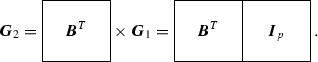 (9.17)
The self-duality of this pure double-circulant code is obvious from \(\varvec{G}_2\).
-
2.
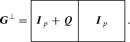
For \(p \equiv -3 \pmod 8\), \((p-1)/2\) is even and hence, neither q(x) nor n(x) is invertible, which means that if this polynomial was chosen as the defining polynomial for \(\mathscr {P}_p\), there exists only one full-rank generator matrix. However, either \(1+q(x)\) (resp. \(1+n(x)\)) is invertible and the inverse is \(1+n(x)\) (resp. \(1+q(x)\)), i.e.
$$\begin{aligned} (1+q(x))(1+n(x))&= 1 + q(x) + n(x) + q(x)n(x)\\&= 1 + q(x) + n(x) + q(x)(1 + j(x) + q(x))\\&= 1 + q(x) + n(x) + q(x) + q(x)j(x) + q(x)^2, \end{aligned}$$and since \(q(x)j(x) = 0\) and \(q(x)^2 = n(x)\) under polynomial modulo \(x^p-1\), it follows that
$$\begin{aligned} (1+q(x))(1+n(x))&= 1 \pmod { x^p-1}. \end{aligned}$$Let \(\varvec{G}_1\) be the first reduced echelon generator matrix, which has the form of (9.5a) where \(\varvec{R}=\varvec{I}_p+\varvec{Q}\). The other full-rank generator matrix with disjoint information sets \(\varvec{G}_2\) can be obtained as follows:
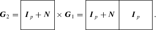 (9.18)
Since \(-1\in Q\) for this prime, \((\varvec{I}_p + \varvec{Q})^T = \varvec{I}_p + \varvec{Q}\) implying that the (2p, p, d) pure double-circulant code is FSD, i.e. the generator matrix of \(\mathscr {P}^\perp _p\) is given by


A bordered double-circulant construction based on these primes—commonly known as the quadratic double-circulant construction—also exists, see Sect. 9.4.3 below.
4.3 Quadratic Double-Circulant Codes
Let p be a prime that is congruent to \(\pm 3\) modulo 8. A \((2(p+1),p+1,d)\) binary quadratic double-circulant code, denoted by \(\mathscr {B}_p\), can be constructed using the defining polynomial
where \(q(x) = \sum _{i\in Q}x^i\). Following [13], the generator matrix \(\varvec{G}\) of \(\mathscr {B}_p\) is

which is, if the last row of \(\varvec{G}\) is rearranged as the first row, the columns indexed by \(l_{\infty }\) and \(r_{\infty }\) are rearranged as the last and the first columns, respectively, equivalent to (9.5b) with \(\alpha =0\) and \(k=p+1\). Let \(j(x)=1+x+x^2+\cdots +x^{p-1}\), and the following are some properties of \(\mathscr {B}_p\) [9]:
-
1.
for \(p\equiv 3 \pmod 8\), \(b(x)^3 = (1+q(x))^2(1+q(x)) = (1+n(x))(1+q(x)) = 1 + j(x)\), since \(q(x)^2 = n(x)\) (\(2\in N\) for this prime) and \(q(x)j(x) = n(x)j(x) = j(x)\) (\(\mathrm {wt}_H(q(x))=\mathrm {wt}_H(n(x))\) is odd). Also, \((b(x)+j(x))^3 = (1+q(x)+j(x))^2(1+q(x)+j(x)) = n(x)^2(1+q(x)+j(x)) = q(x) \,{+}\, n(x) \,{+}\, j(x) \,{=}\, 1\) because \(n(x)^2 = q(x)\). Since \(-1\in N\) and we have \(b(x)^T = 1 + \sum _{i\in Q}x^{-i} = 1 + n(x)\) and thus, \(b(x)b(x)^T = (1+q(x))(1+n(x)) = 1 + j(x)\).
There are two generator full-rank matrices with disjoint information sets for \(\mathscr {B}_p\). This is because, although b(x) has no inverse, \(b(x) + j(x)\) does, and the inverse is \((b(x)+j(x))^2\).
Let \(\varvec{G}_1\) has the form of (9.5b) where \(\varvec{R} = \varvec{B}\), and the other full-rank generator matrix \(\varvec{G}_2\) can be obtained as follows:
$$\begin{aligned} \varvec{G}_2&= \begin{array}{|c|ccc|}\hline 1 &{} 1 &{} \ldots &{} 1\\ \hline 0 &{} &{} &{} \\ \vdots &{} &{} \varvec{B}^T &{} \\ 0 &{} &{} &{} \\ \hline \end{array} \times \varvec{G}_1 = \begin{array}{|c|ccc|c|ccc|}\hline 0 &{} 1 &{} \ldots &{} 1 &{} 1 &{} 0 &{} \ldots &{} 0\\ \hline 1 &{} &{} &{} &{} 0 &{} &{} &{}\\ \vdots &{} &{} \varvec{B}^T &{} &{} \vdots &{} &{} \varvec{I}_p &{}\\ 1 &{} &{} &{} &{} 0 &{} &{} &{}\\ \hline \end{array}\,. \end{aligned}$$(9.21)It is obvious that \(\varvec{G}_2\) is identical to the generator matrix of \(\mathscr {B}^\perp _p\) and hence, it is self-dual.
-
2.
for \(p\equiv -3 \pmod 8\), \(b(x)^3 = n(x)q(x) = (1+j(x)+q(x))q(x) = 1 + j(x)\) since \(q(x)^2 = n(x)\) (\(2\in N\) for this prime) and \(q(x)j(x) = n(x)j(x) = 0\) (\(\mathrm {wt}_H(q(x))=\mathrm {wt}_H(n(x))\) is even). Also, \((b(x) + j(x))^3 = (q(x) + j(x))^2(1 + n(x)) = q(x)^2 + q(x)^2n(x) + j(x)^2 + j(x)^2n(x) = n(x) + q(x) + j(x) = 1\) because \(n(x)^2 = q(x)\). Since \(-1\in Q\) and we have \(b(x)^T = \sum _{i \in Q} x^{-i} = b(x)\) and it follows that \(\mathscr {B}_p\) is FSD, i.e. the generator matrix of \(\mathscr {B}^\perp _p\) is given by
$$\begin{aligned} \varvec{G}^\perp = \begin{array}{|c|ccc|c|ccc|}\hline 0 &{} 1 &{} \ldots &{} 1 &{} 1 &{} 0 &{} \ldots &{} 0\\ \hline 1 &{} &{} &{} &{} 0 &{} &{} &{}\\ \vdots &{} &{} \varvec{B} &{} &{} \vdots &{} &{} \varvec{I}_p &{}\\ 1 &{} &{} &{} &{} 0 &{} &{} &{}\\ \hline \end{array}\, \end{aligned}$$Since \((b(x)+j(x))^{-1} = (b(x)+j(x))^2\), there exist full-rank two generator matrices of disjoint information sets for \(\mathscr {B}_p\). Let \(\varvec{G}_1\) has the form of (9.5b) where \(\varvec{R} = \varvec{B}\), and the other full-rank generator matrix \(\varvec{G}_2\) can be obtained as follows:
$$\begin{aligned} \varvec{G}_2&= \begin{array}{|c|ccc|}\hline 1 &{} 1 &{} \ldots &{} 1\\ \hline 0 &{} &{} &{} \\ \vdots &{} &{} \varvec{B}^2 &{} \\ 0 &{} &{} &{} \\ \hline \end{array} \times \varvec{G}_1 = \begin{array}{|c|ccc|c|ccc|}\hline 0 &{} 1 &{} \ldots &{} 1 &{} 1 &{} 0 &{} \ldots &{} 0\\ \hline 1 &{} &{} &{} &{} 0 &{} &{} &{}\\ \vdots &{} &{} \varvec{B}^2 &{} &{} \vdots &{} &{} \varvec{I}_p &{}\\ 1 &{} &{} &{} &{} 0 &{} &{} &{}\\ \hline \end{array}\, \end{aligned}$$(9.22)
Codes of the form \(\mathscr {B}_p\) form an interesting family of double-circulant codes. In terms of self-dual codes, the family contains the longest extremal Type-II code known, \(n=136\). Probably, it is the longest extremal code that exists, see Sect. 9.7. Moreover, \(\mathscr {B}_p\) is the binary image of the extended QR code over \(\mathbb {F}_4\) [10].
The \((p+1, \frac{1}{2}(p+1), d)\) double-circulant codes for \(p\equiv \pm 1 \pmod 8\) are fixed by \(\text {PSL}_2(p)\), see Sect. 9.4.1. This linear group \(\text {PSL}_2(p)\) is generated by the set of all permutations to the coordinates \(\left( \scriptstyle \infty \displaystyle ,0,1,\ldots ,p-1\right) \) of the form
where \(a,b,c,d \in \mathbb {F}_p\), \(ad - bc = 1\), \(y\in \mathbb {F}_p\cup \{\scriptstyle \infty \displaystyle \}\), and it is assumed that \(\pm \frac{1}{0} = \infty \) and \(\pm \frac{1}{\infty } = 0\) in the arithmetic operations.
We know from [13] that this form of permutation is generated by the following transformations:
where \(\alpha \) is a primitive element of \(\mathbb {F}_p\). In fact, V is redundant since it can be obtained from S and T, i.e.
forFootnote 2 \(\mu = \alpha ^{-1} \in \mathbb {F}_p\).
The linear group \(\text {PSL}_2(p)\) fixes not only the \((p+1, \frac{1}{2}(p+1), d)\) binary double-circulant codes, for \(p\equiv \pm 1 \pmod 8\), but also the \((2(p+1), p+1, d)\) binary quadratic double-circulant codes, as shown as follows. Consider the coordinates \(\left( \scriptstyle \infty \displaystyle ,0,1,\ldots ,p-1\right) \) of a circulant, the transformation S leaves the coordinate \({\scriptstyle \infty \displaystyle }\) invariant and introduces a cyclic shift to the rest of the coordinates and hence S fixes a circulant. Let \(\varvec{R}_i\) and \(\varvec{L}_i\) denote the ith row of the right and left circulants of (9.20), respectively (we assume that the index starts with 0), and let \(\varvec{J}\) and \(\varvec{J}^\prime \) denote the last row of the right and left circulant of (9.20), respectively.
Consider the primes \(p = 8m + 3\), \(\varvec{R}_0 = \left( 0 \mid 1+\sum _{i \in Q}x^i\right) \). Let \(e_i\) and \(f_j\), for some integers i and j, be even and odd integers, respectively. If \(i\in Q\), \(-1/i = -1 \times \alpha ^{p-1}/\alpha ^{e_1} = \alpha ^{f_1}\times \alpha ^{e_2 - e_1} \in N\) since \(-1\in N\) for these primes. Therefore, the transformation T interchanges residues to non-residues and vice versa. In addition, we also know that T interchanges coordinates \(\infty \) and 0. Applying transformation T to \(\varvec{R}_0\), \(T(\varvec{R}_0)\), results in
Similarly, for the first row of \(\varvec{L}\), which has 1 at coordinates \(\infty \) and 0 only, i.e. \(\varvec{L}_0 = (1 \mid 1)\)
Let \(s\in Q\) and let the set \(\hat{Q} = Q \cup \{0\}\), \(\varvec{R}_s = \left( 0 \mid \sum _{i \in \hat{Q}} x^{s + i}\right) \) and \(T\left( \sum _{i \in \hat{Q}} x^{s + i}\right) = \sum _{i\in \hat{Q}} x^{-1/(s+i)}\). Following MacWilliams and Sloane [13, Theorem 24, Chap. 16], we know that the exponents of \(\sum _{i \in \hat{Q}} x^{s + i}\) contain \(2m+1\) residues and \(2m+1\) non-residues. Note that \(s+i\) produces no 0.Footnote 3 It follows that \(-1/(s + i)\) contains \(2m + 1\) non-residues and \(2m + 1\) residues. Now consider \(\varvec{R}_{-1/s} = \left( 0 \mid \sum _{i \in \hat{Q}} x^{i - 1/s}\right) \), \(i - 1/s\) containsFootnote 4 0 \(i,s\in Q\), 2m residues and \(2m + 1\) non-residues. We can write \(-1/(s+i)\) as
Let \(I \subset \hat{Q}\) be a set of all residues such that for all \(i \in I\), \(i - 1/s \in N\). If \(-1/(s+i) \in ~N\), \(z \in \hat{Q}\) and we can see that z must belong to I such that \(z - 1/s \in N\). This means these non-residues cancel each other in \(T(\varvec{R}_s) + \varvec{R}_{-1/s}\). On the other hand, if \(-1/(s+i) \in Q\), \(z \in N\) and it is obvious that \(z - 1/s \ne i - 1/s\) for all \(i\in \hat{Q}\), implying that all \(2m + 1\) residues in \(T(\varvec{R}_s)\) are disjoint from all \(2m + 1\) residues (including 0) in \(\varvec{R}_{-1/s}\). Therefore, \(T(\varvec{R}_s) + \varvec{R}_{-1/s} = \left( 0 \mid \sum _{i \in \hat{Q}} x^i\right) \), i.e.
Similarly, \(T(\varvec{L}_s) = \left( 0 \mid 1 + x^{-1/s}\right) \) and \(\varvec{L}_{-1/s} = \left( 1 \mid x^{-1/s}\right) \), which means
Let \(t \in N\), \(\varvec{R}_t = \left( 0 \mid \sum _{i\in \hat{Q}} x^{t + i}\right) \) and \(T\left( \sum _{i \in \hat{Q}} x^{t+i}\right) = \sum _{i \in \hat{Q}} x^{-1/(t + i)}\). We know that \(t + i\) contains 0, 2m residues and \(2m + 1\) non-residues [13, Theorem 24, Chap. 16], and correspondingly \(-1/(t+i)\) contains \(\infty \), 2m non-residues and \(2m + 1\) residues. As before, now consider \(\varvec{R}_{-1/t} = \left( 0 \mid \sum _{i \in \hat{Q}} x^{i - 1/t} \right) \). There are \(2m + 1\) residues (excluding 0) and \(2m + 1\) non-residues in \(i - 1/t\), and let \(I^\prime \subset \hat{Q}\) be a set of all residues such that, for all \(i \in I^\prime \), \(i - 1/t \in Q\). As before, we can write \(-1/(t + i)\) as \(z - 1/t\), where \(z = (i/t)/(t+i)\). If \(-1/(t+i) \in Q\), \(z \in I^\prime \) and hence, the \(2m + 1\) residues from \(-1/(t+i)\) are identical to those from \(i - 1/t\). If \(-1/(t+i) \in N\), \(z \in N\) and hence, all of the 2m non-residues of \(-1/(t+i)\) are disjoint from all \(2m+1\) non-residues of \(i - 1/t\). Therefore, \(T(\varvec{R}_t) + R_{-1/t} = \left( 1 \mid \sum _{i \in N} x^i\right) \), i.e.
Similarly, \(T(\varvec{L}_t) = \left( 0 \mid 1 + x^{-1/t}\right) \) and \(\varvec{L}_{-1/t} = \left( 1 \mid x^{-1/t}\right) \), which means
For primes \(p = 8m - 3\), \(\varvec{R}_0 = \left( 0 \mid \sum _{i \in Q} x^i \right) \) and since \(-1 \in Q\), \(-1/i \in Q\) for \(i \in Q\). Thus,
Similarly, for \(\varvec{L}_0\), which contains 1 at coordinates 0 and \(\infty \),
Consider \(\varvec{R}_s = \left( 0 \mid \sum _{i \in Q} x^{s + i} \right) \), for \(s \in Q\), \(T\left( \sum _{i \in Q} x^{s + i}\right) = \sum _{i \in Q} x^{-1/(s+i)}\). There are 0 (when \(i = -s\in Q\)), \(2m-2\) residues and \(2m - 1\) non-residues in the set \(s + i\) [13, Theorem 24, Chap. 16]. Correspondingly, \(-1/(s+i) = z - 1/s\), where \(z = (i/s)/(s+i)\), contains \(\infty \), \(2m-2\) residues and \(2m-1\) non-residues. Now consider \(\varvec{R}_{-1/s} = \left( 0 \mid \sum _{i \in Q} x^{i - 1/s} \right) \), the set \(i - 1/s\) contains 0 (when \(i = 1/s \in Q\)), \(2m-2\) residues and \(2m-1\) non-residues. Let \(I \subset Q\) be a set of all residues such that for all \(i\in I\), \(i - 1/s \in Q\). If \(-1/(s + i) \in Q\) then \(z - 1/s \in Q\) which means \(z \in Q\) and z must belong to I. This means all \(2m-2\) residues of \(-1/(s+i)\) and those of \(i - 1/s\) are identical. On the contrary, if \(-1/(s + i) \in N\), \(z \in N\) and this means \(z - 1/s \ne i - 1/s\) for all \(i \in Q\), and therefore all non-residues in \(-1/(s+i)\) and \(i - 1/s\) are mutually disjoint. Thus, \(T(\varvec{R}_s) + \varvec{R}_{-1/s} = \left( 1 \mid 1 + \sum _{i \in N} x^i \right) \), i.e.
Similarly, \(T(\varvec{L}_s) = \left( 0 \mid 1 + x^{-1/s} \right) \), and we can write
For \(t \in N\), we have \(\varvec{R}_t = \left( 0 \mid \sum _{i \in Q} x^{t + i} \right) \) and \(T(\sum _{i\in Q} x^{t + i}) = \sum _{i \in Q} x^{-1/(t+i)}\). Following [13, Theorem 24, Chap. 16], there are \(2m-1\) residues and \(2m-1\) non-residues in the set \(t+i\) and the same distributions are contained in the set \(-1/(t+i)\). Considering \(\varvec{R}_{-1/t} = \left( 0 \mid \sum _{i\in Q} x^{i-1/t}\right) \), there are \(2m-1\) residues and \(2m-1\) non-residues in \(i - 1/t\). Rewriting \(-1/(t+i) = z - 1/t\), for \(z = (i/t)/(t+i)\), and letting \(I^\prime \subset Q\) be a set of all residues such that for all \(i \in I^\prime \), \(i - 1/t \in N\), we know that if \(-1/(t+i) \in N\) then \(z - 1/t\in N\) which means that \(z\in Q\) and z must belong to \(I^\prime \). Hence, the non-residues in \(i - 1/t\) and \(-1/(t+i)\) are identical. If \(-1/(t+i) \in Q\), however, \(z \in N\) and for all \(i \in Q\), \(i - 1/t \ne z - 1/t\), implying that the residues in \(-1/(t+i)\) and \(i - 1/t\) are mutually disjoint. Thus, \(T(\varvec{R}_t) + \varvec{R}_{-1/t} = \left( 0 \mid \sum _{i\in Q}x^i\right) \), i.e.
Similarly, \(T(\varvec{L}_t) = \left( 0 \mid 1 + x^{-1/t} \right) \), and we can write
The effect T to the circulants is summarised as follows:

where \(s\in Q\) and \(t\in N\). This shows that, for \(p\equiv \pm 3 \pmod 8\), the transformation T is a linear combination of at most three rows of the circulant and hence it fixes the circulant. This establishes the following theorem on \(\text {Aut}(\mathscr {B}_p)\) [2, 13].
Theorem 9.1
The automorphism group of the \((2(p+1),p+1,d)\) binary quadratic double-circulant codes contains \(\text {PSL}_2(p)\) applied simultaneously to both circulants.
The knowledge of \(\text {Aut}(\mathscr {B}_p)\) can be exploited to deduce the modular congruence weight distributions of \(\mathscr {B}_p\) as shown in Sect. 9.6.
5 Evaluation of the Number of Codewords of Given Weight and the Minimum Distance: A More Efficient Approach
In Chap. 5 algorithms to compute the minimum distance of a binary linear code and to count the number of codewords of a given weight are described. Assuming the code rate of the code is a half and its generator matrix contains two mutually disjoint information sets, each of rank k (the code dimension), these algorithms require enumeration of
codewords in order to count the number of codewords of weight w. For FSD double-circulant codes with \(p\equiv -3 \pmod 8\) and self-dual double-circulant codes a more efficient approach exists. This approach applies to both pure and bordered double-circulant cases.
Lemma 9.7
Let \(T_m(x)\) be a set of binary polynomials with degree at most m. Let \(u_i(x),v_i(x) \in T_{k-1}(x)\) for \(i=1,2\), and \(e(x),f(x) \in T_{k-2}(x)\). The numbers of weight w codewords of the form \(c_1(x) = (u_1(x)|v_1(x))\) and \(c_2(x) = (v_2(x)|u_2(x))\) are equal, where
-
(i)
for self-dual pure double-circulant codes, \(u_2(x) = u_1(x)^T\) and \(v_2(x) = v_1(x)^T\);
-
(ii)
for self-dual bordered double-circulant codes, \(u_1(x) = (\varepsilon | e(x))\), \(v_1(x) = (\gamma | f(x))\), \(u_2(x) = (\varepsilon | e(x)^T)\) and \(v_2(x) = (\gamma | f(x)^T)\), where \(\gamma = \mathrm {wt}_H(e(x)) \pmod 2\);
-
(iii)
for FSD pure double-circulant codes (\(p\equiv -3 \pmod 8\)), \(u_2(x) = u_1(x)^2\) and \(v_2(x) = v_1(x)^2\);
-
(iv)
for FSD bordered double-circulant codes (\(p\equiv -3 \pmod 8\)), \(u_1(x) {=} (\varepsilon |e(x))\), \(v_1(x) = (\gamma |f(x))\), \(u_2(x) = (\varepsilon |e(x)^2)\), \(v_2(x) = (\gamma |f(x)^2)\), where \(\gamma = \mathrm {wt}_H(e(x)) \pmod 2\).
Proof
-
(i)
Let \(\varvec{G}_1 = [\varvec{I}_k | \varvec{R}]\) and \(\varvec{G}_2 = [\varvec{R}^T | \varvec{I}_k]\) be the two full-rank generator matrices with mutually disjoint information sets of a self-dual pure double-circulant code. Assume that r(x) and \(r(x)^T\) are the defining polynomials of \(\varvec{G}_1\) and \(\varvec{G}_2\), respectively. Given \(u_1(x)\) as an input, we have a codeword \(c_1(x) = (u_1(x) | v_1(x))\), where \(v_1(x) = u_1(x)r(x)\), from \(\varvec{G}_1\). Another codeword \(c_2(x)\) can be obtained from \(\varvec{G}_2\) using \(u_1(x)^T\) as an input, \(c_2(x) = (v_1(x)^T | u_1(x)^T)\), where \(v_1(x)^T = u_1(x)^Tr(x)^T = (u_1(x)r(x))^T\). Since the weight of a polynomial and that of its transpose are equal, for a given polynomial of degree at most \(k-1\), there exist two distinct codewords of the same weight.
-
(ii)
Let \(\varvec{G}_1\), given by (9.5b), and \(\varvec{G}_2\) be two full-rank generator matrices with pairwise disjoint information sets, of bordered self-dual double-circulant codes. It is assumed that the form of \(\varvec{G}_2\) is identical to that given by (9.21) with \(\varvec{R}^T=\varvec{B}^T\). Let \(f(x) = e(x)r(x)\), consider the following cases:
-
a.
\(\varepsilon = 0\) and \(\mathrm {wt}_H(e(x))\) is odd, we have a codeword \(c_1(x) = \left( 0 \mid e(x) \mid 1 \mid \right. \left. f(x)\right) \) from \(\varvec{G}_1\). Applying \(\left( 0 \mid e(x)^T \right) \) as an information vector to \(\varvec{G}_2\), we have another codeword \(c_2(x) = \left( 1 \mid e(x)^Tr(x)^T \mid 0 \mid e(x)^T \right) = \left( 1 \mid f(x)^T \right. \) \(\left. \mid 0 \mid e(x)^T\right) \).
-
b.
\(\varepsilon \,{=}\, 1\) and \(\mathrm {wt}_H(e(x))\) is odd, \(\varvec{G}_1\) produces \(c_1(x) \,{=}\, \left( \! 1 \mid e(x) \mid 1 \mid \right. \left. f(x) \,{+}\, j(x)\! \right) \). Applying \(\left( 1 \mid e(x)^T\right) \) as an information vector to \(\varvec{G}_2\), we have a codeword \(c_2(x) \,{=}\, \left( 1 \mid e(x)^Tr(x)^T \,{+}\, j(x) \mid 1 \mid e(x)^T \right) \,{=}\, \left( 1 \mid f(x)^T \,{+} \right. \) \(\left. j(x) \mid 1 \mid e(x)^T\right) \).
-
c.
\(\varepsilon = 0\) and \(\mathrm {wt}_H(e(x))\) is even, \(\varvec{G}_1\) produces a codeword \(c_1(x) = \left( 0 \mid e(x) \mid 0 \mid \right. \) \(\left. f(x) \right) \). Applying \(\left( 0 \mid e(x)^T\right) \) as an information vector to \(\varvec{G}_2\), we have another codeword \(c_2(x) = \left( 0 \mid e(x)^Tr(x)^T \mid 0 \mid e(x)^T \right) = \left( 0 \mid f(x)^T \mid 0 \mid e(x)^T\right) \).
-
d.
\(\varepsilon = 1\) and \(\mathrm {wt}_H(e(x))\) is even, \(\varvec{G}_1\) produces \(c_1(x) = \left( 1 \mid e(x) \mid 0 \mid f(x)+\right. \) \(\left. j(x) \right) \). Applying \(\left( 1 \mid e(x)^T\right) \) as an information vector to \(\varvec{G}_2\), we have a codeword \(c_2(x) = \left( 0 \mid e(x)^Tr(x)^T + j(x) \mid 1 \mid e(x)^T \right) = \left( 0 \mid f(x)^T + j(x) \right. \) \(\left. \mid 1 \mid e(x)^T\right) \).
It is clear that in all cases, \(\mathrm {wt}_H(c_1(x)) = \mathrm {wt}_H(c_2(x))\) since \(\mathrm {wt}_H(v(x)) = \mathrm {wt}_H(v(x)^T)\) and \(\mathrm {wt}_H(v(x)+j(x)) = \mathrm {wt}_H(v(x)^T+j(x))\) for some polynomial v(x). This means that given an information vector, there always exist two distinct codewords of the same weight.
-
a.
-
(iii)
Let \(\varvec{G}_1\), given by (9.5a) with \(\varvec{R}=\varvec{I}_p + \varvec{Q}\), and \(\varvec{G}_2\), given by (9.18), be two full-rank generator matrices with pairwise disjoint information sets, of pure FSD double-circulant codes for \(p\equiv -3 \pmod 8\).
Given \(u_1(x)\) as input, we have a codeword \(c_1(x) = (u_1(x) | v_1(x))\), where \(v_1(x) = u_1(x)(1+q(x))\), from \(\varvec{G}_1\) and another codeword \(c_2(x) = (v_2(x) | u_2(x))\), where \(u_2(x) = u_1(x)^2\) and \(v_2(x) = u_1(x)^2(1+n(x)) = u_1(x)^2(1\) \(+q(x))^2 = v_1(x)^2\), from \(\varvec{G}_2\). Since the weight of a polynomial and that of its square are the same over \(\mathbb {F}_2\), the proof follows.
-
(iv)
Let \(\varvec{G}_1\), given by (9.5b) with \(\varvec{B}=\varvec{R}\), and \(\varvec{G}_2\), given by (9.22), be two full-rank generator matrices with pairwise disjoint information sets, of bordered FSD double-circulant codes for \(p\equiv -3 \pmod 8\). Let \(f(x) = e(x)b(x)\), consider the following cases:
-
a.
\(\varepsilon = 0\) and \(\mathrm {wt}_H(e(x))\) is odd, we have a codeword \(c_1(x) {=} \left( 0 \mid e(x) \mid 1 \mid f(x)\right) \) from \(\varvec{G}_1\). Applying \(\left( 0 \mid e(x)^2 \right) \) as an information vector to \(\varvec{G}_2\), we have another codeword \(c_2(x) = \left( 1 \mid e(x)^2n(x) \mid 0 \mid e(x)^2 \right) \). Since \(e(x)^2n(x) = e(x)^2b(x)^2 = f(x)^2\), the codeword \(c_2 = \left( 1 \mid f(x)^2 \mid 0 \mid e(x)^2 \right) \).
-
b.
\(\varepsilon = 1\) and \(\mathrm {wt}_H(e(x))\) is odd, \(\varvec{G}_1\) produces \(c_1(x) = \left( 1 \mid e(x) \mid 1 \mid f(x)\right. \) \(\left. + j(x) \right) \). Applying \(\left( 1 \mid e(x)^2\right) \) as an information vector to \(\varvec{G}_2\), we have a codeword \(c_2(x) = \left( 1 \mid e(x)^2n(x) + j(x) \mid 1 \mid e(x)^2 \right) = \left( 1 \mid f(x)^2 + j(x) \right. \) \(\mid \left. 1 \mid e(x)^2\right) \).
-
c.
\(\varepsilon = 0\) and \(\mathrm {wt}_H(e(x))\) is even, \(\varvec{G}_1\) produces a codeword \(c_1(x) = \left( 0 \mid e(x) \mid 0\right. \) \(\left. \mid f(x) \right) \). Applying \(\left( 0 \mid e(x)^2\right) \) as an information vector to \(\varvec{G}_2\), we have another codeword \(c_2(x) = \left( 0 \mid e(x)^2n(x) \mid 0 \mid e(x)^2 \right) = \left( 0 \mid f(x)^2 \mid 0 \right. \) \(\mid \left. e(x)^2\right) \).
-
d.
\(\varepsilon = 1\) and \(\mathrm {wt}_H(e(x))\) is even, \(\varvec{G}_1\) produces \(c_1(x) = \left( 1 \mid e(x) \mid 0 \mid f(x)\right. \) \(\left. + j(x) \right) \). Applying \(\left( 1 \mid e(x)^2\right) \) as an information vector to \(\varvec{G}_2\), we have a codeword \(c_2(x) = \left( 0 \mid e(x)^2n(x) + j(x) \mid 1 \mid e(x)^2 \right) = \left( 0 \mid f(x)^2 + j(x)\right. \) \(\left. \mid 1 \mid e(x)^2\right) \).
It is clear that in all cases, \(\mathrm {wt}_H(c_1(x)) = \mathrm {wt}_H(c_2(x))\) since \(\mathrm {wt}_H(v(x)) = \mathrm {wt}_H(v(x)^2)\) and \(\mathrm {wt}_H(v(x)+j(x)) = \mathrm {wt}_H(v(x)^2+j(x))\) for some polynomial v(x). This means that given an information vector, there always exist two distinct codewords of the same weight.
-
a.
From Lemma 9.7, it follows that, in order to count the number of codewords of weight w, we only require
codewords to be enumerated and if \(A_w\) denotes the number of codewords of weight w,
where \(a_i\) is the number of weight w codewords which have i non-zeros in the first k coordinates.
Similarly, the commonly used method to compute the minimum distance of half-rate codes with two full-rank generator matrices of mutually disjoint information sets, for example, see van Dijk et al. [18], assuming that d is the minimum distance of the code, requires as many as
codewords to be enumerated. Following Lemma 9.7, only S / 2 codewords are required for \(\mathscr {P}_p\) and \(\mathscr {B}_p\) for \(p\equiv -3 \pmod 8\), and self-dual double-circulant codes. Note that the bound \(d/2 - 1\) may be improved for singly even and doubly even codes, but we consider the general case here.
6 Weight Distributions
The automorphism group of both \((p+1,\frac{1}{2}(p+1),d)\) extended QR and \((2(p+1),p+1,d)\) quadratic double-circulant codes contains the projective special linear group, \(\text {PSL}_2(p)\). Let \(\mathscr {H}\) be a subgroup of the automorphism group of a linear code, and the number of codewords of weight i, denoted by \(A_i\), can be categorised into two classes:
-
1.
a class of weight i codewords which are invariant under some element of \(\mathscr {H}\); and
-
2.
a class of weight i codewords which forms an orbit of size \(|\mathscr {H}|\), the order of \(\mathscr {H}\). In the other words, if \(\varvec{c}\) is a codeword of this class, applying all elements of \(\mathscr {H}\) to \(\varvec{c}\), \(|\mathscr {H}|\) distinct codewords are obtained.
Thus, we can write \(A_i\) in terms of congruence as follows:
where \(A_i(\mathscr {H})\) is the number of codewords of weight i fixed by some element of \(\mathscr {H}\). This was originally shown by Mykkeltveit et al. [14], where it was applied to extended QR codes for primes 97 and 103.
6.1 The Number of Codewords of a Given Weight in Quadratic Double-Circulant Codes
For \(\mathscr {B}_p\), we shall choose \(\mathscr {H}=\text {PSL}_2(p)\), which has order \(|\mathscr {H}|=\frac{1}{2}p(p^2-1)\). Let the matrix \(\bigl [{\begin{matrix}a &{} b\\ c &{} d\end{matrix}}\bigr ]\) represent an element of \(\text {PSL}_2(p)\), see (9.23). Since \(|\mathscr {H}|\) can be factorised as \(|\mathscr {H}|=\prod _{j}q_j^{e_j}\), where \(q_j\) is a prime and \(e_j\) is some integer, \(A_i(\mathscr {H}) \pmod { |\mathscr {H}|}\) can be obtained by applying the Chinese remainder theorem to \(A_i(S_{q_j}) \pmod { q_j^{e_j}}\) for all \(q_j\) that divides \(|\mathscr {H}|\), where \(S_{q_j}\) is the Sylow-\(q_j\)-subgroup of \(\mathscr {H}\). In order to compute \(A_i(S_{q_j})\), a subcode of \(\mathscr {B}_p\) which is invariant under \(S_{q_j}\) needs to be obtained in the first place. This invariant subcode, in general, has a considerably smaller dimension than \(\mathscr {B}_p\), and hence, its weight distribution can be easily obtained.
For each odd prime \(q_j\), \(S_{q_j}\) is a cyclic group which can be generated by some \(\bigl [{\begin{matrix}a&{}b\\ c&{}d\end{matrix}}\bigr ]\in \text {PSL}_2(p)\) of order \(q_j\). Because \(S_{q_j}\) is cyclic, it is straightforward to obtain the invariant subcode, from which we can compute \(A_i(S_{q_j})\).
On the other hand, the case of \(q_j=2\) is more complicated. For \(q_j=2\), \(S_{2}\) is a dihedral group of order \(2^{m+1}\), where \(m+1\) is the maximum power of 2 that divides \(|\mathscr {H}|\) [14]. For \(p=8m \pm 3\), we know that
which shows that the highest power of 2 that divides \(|\mathscr {H}|\) is \(2^2\) (\(m=1\)). Following [14], there are \(2^m + 1\) subgroups of order 2 in \(S_2\), namely
where \(P,T\in \text {PSL}_2(p)\), \(P^2\ = T^2 = 1\) and \(TPT^{-1} = P^{-1}\).
Let \(T = \bigl [{\begin{matrix}0&{}p-1\\ 1&{}0\end{matrix}}\bigr ]\), which has order 2. It can be shown that any order 2 permutation, \(P = \bigl [{\begin{matrix}a&{}b\\ c&{}d\end{matrix}}\bigr ]\), if a constraint \(b=c\) is imposed, we have \(a=-d\). All these subgroups, however, are conjugates in \(\text {PSL}_2(p)\) [14] and therefore, the subcodes fixed by \(G^0_2\), \(G^1_2\) and \(H_2\) have identical weight distributions and considering any of them, say \(G^0_2\), is sufficient.
Apart from \(2^m + 1\) subgroups of order 2, \(S_2\) also contains a cyclic subgroup of order 4, \(2^{m-1}\) non-cyclic subgroups of order 4, and subgroups of order \(2^j\) for \(j \ge 3\).
Following [14], only the subgroups of order 2 and the non-cyclic subgroups of order 4 make contributions towards \(A_i(S_2)\). For \(p\equiv \pm 3 \pmod 8\), there is only one non-cyclic subgroup of order 4, denoted by \(G_4\), which contains, apart from an identity, three permutations of order 2 [14], i.e. a Klein 4 group,
Having obtained \(A_i(G^0_2)\) and \(A_i(G_4)\), following the argument in [14], the number of codewords of weight i that are fixed by some element of \(S_2\) is given by
In summary, in order to deduce the modular congruence of the number of weight i codewords in \(\mathscr {B}_p\), it is sufficient to do the following steps:
-
1.
compute the number of weight i codewords in the subcodes fixed by \(G^0_2\), \(G_4\) and \(S_q\), for all odd primes q that divide \(|\mathscr {H}|\);
-
2.
apply (9.28) to \(A_i(G^0_2)\) and \(A_i(G_4)\) to obtain \(A_i(S_2)\); and then
-
3.
apply the Chinese remainder theorem to \(A_i(S_2)\) and all \(A_i(S_q)\) to obtain \(A_i(\mathscr {H}) \pmod { |\mathscr {H}|}\).
Given \(\mathscr {B}_p\) and an element of \(\text {PSL}_2(p)\), how can we find the subcode consisting of the codewords fixed by this element? Assume that \(Z = \bigl [{\begin{matrix}a&{}b\\ c&{}d\end{matrix}}\bigr ] \in \text {PSL}_2(p)\) of prime order. Let \(c_{l_i}\) (resp. \(c_{r_i}\)) and \(c_{l_{i^\prime }}\) (resp. \(c_{r_{i^\prime }}\)) denote the ith coordinate and \(\pi _Z(i)\)th coordinate (ith coordinate with the respect to permutation \(\pi _Z\)), in the left (resp. right) circulant form, respectively. The invariant subcode can be obtained by solving a set of linear equations consisting of the parity-check matrix of \(\mathscr {B}_p\) (denoted by \(\varvec{H}\)), \(c_{l_i} + c_{l_{i^\prime }} = 0\) (denoted by \({\varvec{\pi }}_Z(L)\)) and \(c_{r_i} + c_{r_{i^\prime }} = 0\) (denoted by \({\varvec{\pi }}_Z(R)\)) for all \(i\in \mathbb {F}_p~\cup ~\{\scriptstyle \infty \displaystyle \}\), i.e.
The solution to \(\varvec{H}_{sub}\) is a matrix of rank \(r > (p+1)\), which is the parity-check matrix of the \((2(p+1), 2(p+1)-r, d^\prime )\) invariant subcode. For subgroup \(G_4\), which consists of permutations P, T and PT, we need to solve the following matrix
to obtain the invariant subcode. Note that the parity-check matrix of \(\mathscr {B}_p\) is assumed to have the following form:

One useful application of the modular congruence of the number of codewords of weight w is to verify, independently, the number of codewords of a given weight w that were computed exhaustively.
Computing the number of codewords of a given weight in small codes using a single-threaded algorithm is tractable, but for longer codes, it is necessary to use multiple computers working in parallel to produce a result within a reasonable time. Even so it can take several weeks, using hundreds of computers, to evaluate a long code. In order to do the splitting, the codeword enumeration task is distributed among all of the computers and each computer just needs to evaluate a predetermined number of codewords, finding the partial weight distributions. In the end, the results are combined to give the total number of codewords of a given weight. There is always the possibility of software bugs or mistakes to be made, particularly in any parallel computing scheme. The splitting may not be done correctly or double-counting or miscounting introduced as a result, apart from possible errors in combining the partial results. Fortunately, the modular congruence approach can also provide detection of computing errors by revealing inconsistencies in the summed results. The importance of this facet of modular congruence will be demonstrated in determining the weight distributions of extended QR codes in Sect. 9.6.2. In the following examples we work through the application of the modular congruence technique in evaluating the weight distributions of the quadratic double-circulant codes of primes 37 and 83.
Example 9.1
For prime 37, there exists an FSD (76, 38, 12) quadratic double-circulant code, \(\mathscr {B}_{37}\). The weight enumerator of an FSD code is given by Gleason’s theorem [15]
for integers \(K_i\). The number of codewords of any weight w is given by the coefficient of \(z^w\) of A(z). In order to compute A(z) of \(\mathscr {B}_{37}\), we need only to compute \(A_{2i}\) for \(6\le i \le 9\). Using the technique described in Sect. 9.5, the number of codewords of desired weights is obtained and then substituted into (9.30). The resulting weight enumerator function giving the whole weight distribution of the (76, 38, 12) code, \(\mathscr {B}_{37}\) is
Let \(\mathscr {H} = \text {PSL}_2(37)\), and we know that \(|\mathscr {H}|= 2^2\times 3^2\times 19\times 37=25308\). Consider the odd primes as factors q. For \(q = 3\), \(\bigl [{\begin{matrix}0&{}1\\ 36&{}1\end{matrix}}\bigr ]\) generates the following permutation of order 3:
The corresponding invariant subcode has a generator matrix \(G^{(S_3)}\) of dimension 14, which is given by

and its weight enumerator function is
For \(q = 19\), \(\bigl [{\begin{matrix}0&{}1\\ 36&{}3\end{matrix}}\bigr ]\) generates the following permutation of order 19:
The resulting generator matrix of the invariant subcode \(\varvec{G}^{(S_{19})}\), which has dimension 2, is
and its weight enumerator function is
For the last odd prime, \(q=37\), a permutation of order 37
is generated by \(\bigl [{\begin{matrix}0&{}1\\ 36&{}35\end{matrix}}\bigr ]\) and it turns out that the corresponding invariant subcode, and hence, the weight enumerator function, are identical to those of \(q=19\).
For \(q=2\), subcodes fixed by some element of \(G^0_2\) and \(G_4\) are required. We have \(P=\bigl [{\begin{matrix}3&{}8\\ 8&{}34\end{matrix}}\bigr ]\) and \(T=\bigl [{\begin{matrix}0&{}36\\ 1&{}0\end{matrix}}\bigr ]\), and the resulting order 2 permutations generated by P, T and PT are
and
respectively. It follows that the corresponding generator matrices and weight enumerator functions of the invariant subcodes are

which has dimension 20, with
and

which has dimension 12, with
respectively. Consider the number of codewords of weight 12, from (9.31)−(9.35), we know that \(A_{12}(G^0_2)=21\) and \(A_{12}(G_4)=3\); applying (9.28),
and thus, we have the following set of simultaneous congruences:
Following the Chinese remainder theorem, a solution to the above congruences, denoted by \(A_{12}(\mathscr {H})\), is congruent modulo \({{\mathrm{LCM}}}\{2^2,3^2,19,37\}\), where \({{\mathrm{LCM}}}\{2^2,3^2,19, 37\}\) is the least common multiple of the moduli \(2^2\), \(3^2\), 19 and 37, which is equal to \(2^2\times 3^2\times 19\times 37=25308\) in this case. Since these moduli are pairwise coprime, by the extended Euclidean algorithm, we can write
A solution to the congruences above is given by
Referring to the weight enumerator function, (9.31), we can immediately see that \(n_{12}=0\), indicating that \(A_{12}\) has been accurately evaluated. Repeating the above procedures for weights larger than 12, we have Table 9.3 which shows that the weight distributions of \(\mathscr {B}_{37}\) are indeed accurate. In fact, since the complete weight distributions can be obtained once the first few terms required by Gleason’s theorem are known, verification of these few terms is sufficient.
Example 9.2
Gulliver et al. [6] have shown that the (168, 84, 24) doubly even self-dual quadratic double-circulant code \(\mathscr {B}_{83}\) is not extremal since it has minimum distance less than or equal to 28. The weight enumerator of a Type-II code of length n is given by Gleason’s theorem, which is expressed as [15]
where \(K_i\) are some integers. As shown by (9.36), only the first few terms of \(A_i\) are required in order to completely determine the weight distribution of a Type-II code. For \(\mathscr {B}_{83}\), only the first eight terms of \(A_i\) are required. Using the parallel version of the efficient codeword enumeration method described in Chap. 5, Sect. 9.5, we determined that all of these eight terms are 0 apart from \(A_0=1\), \(A_{24}=571704\) and \(A_{28}=17008194\).
We need to verify independently whether or not \(A_{24}\) and \(A_{28}\) have been correctly evaluated. As in the previous example, the modular congruence method can be used for this purpose. For \(p = 83\), we have \(|\mathscr {H}|=2^2\times 3\times 7\times 41\times 83=285852\). We will consider the odd prime cases in the first place.
For prime \(q=3\), a cyclic group of order 3, \(S_3\) can be generated by \(\bigl [{\begin{matrix} 0&{}1\\ 82&{}1\end{matrix}}\bigr ]\in \text {PSL}_2(83)\), and we found that the subcode invariant under \(S_3\) has dimension 28 and has 63 and 0 codewords of weights 24 and 28, respectively.
For prime \(q=7\), we have \(\bigl [{\begin{matrix} 0&{}1\\ 82&{}10\end{matrix}}\bigr ]\) which generates \(S_7\). The subcode fixed by \(S_7\) has dimension 12 and no codewords of weight 24 or 28 are contained in this subcode.
Similarly, for prime \(q=41\), the subcode fixed by \(S_{41}\), which is generated by \(\bigl [{\begin{matrix} 0&{}1\\ 82&{}4\end{matrix}}\bigr ]\) and has dimension 4, contains no codewords of weight 24 or 28.
Finally, for prime \(q=83\), the invariant subcode of dimension 2 contains the all-zeros, the all-ones, \(\{\underbrace{0,0,\ldots ,0,0}_{84},\underbrace{1,1,\ldots ,1,1}_{84}\}\) and \(\{\underbrace{1,1,\ldots ,1,1}_{84},\underbrace{0,0,\ldots ,0,0}_{84}\}\) codewords only. The cyclic group \(S_{83}\) is generated by \(\bigl [{\begin{matrix} 0&{}1\\ 82&{}81\end{matrix}}\bigr ]\).
For the case of \(q=2\), we have \(P=\bigl [{\begin{matrix}1 &{} 9\\ 9 &{} 82\end{matrix}}\bigr ]\) and \(T=\bigl [{\begin{matrix}0 &{}82\\ 1 &{} 0\end{matrix}}\bigr ]\). The subcode fixed by \(S_2\), which has dimension 42, contains 196 and 1050 codewords of weights 24 and 28, respectively. Meanwhile, the subcode fixed by \(G_4\), which has dimension 22, contains 4 and 6 codewords of weights 24 and 28, respectively.
Thus, using (9.28), the numbers of codewords of weights 24 and 28 fixed by \(S_2\) are
and by applying the Chinese remainder theorem to all \(A_i(S_q)\) for \(i=24,28\), we arrive at
and
From (9.2) we have now verified \(A_{24}\) and \(A_{28}\), since they have equality for non-negative integers \(n_{24}\) and \(n_{28}\) (\(n_{24}=2\) and \(n_{28}=59\)). Using Gleason’s theorem, i.e. (9.36), the weight enumerator function of the (168, 84, 24) code \(\mathscr {B}_{83}\) is obtained and it is given by
For the complete weight distributions and their congruences of the \((2(p+1), p+1, d)\) quadratic double-circulant codes, for \(11 \le p \le 83\), except \(p=37\) as it has already been given in Example 9.1, refer to Appendix “Weight Distributions of Quadratic Double-Circulant Codes and their Modulo Congruence”.
6.2 The Number of Codewords of a Given Weight in Extended Quadratic Residue Codes
We have modified the modular congruence approach of Mykkeltveit et al. [14], which was originally introduced for extended QR codes \(\mathscr {\hat{L}}_p\), so that it is applicable to the quadratic double-circulant codes. Whilst \(\mathscr {B}_p\) contains one non-cyclic subgroup of order 4, \(\mathscr {\hat{L}}_p\) contains two distinct non-cyclic subgroups of this order, namely \(G^0_4\) and \(G^1_4\). As a consequence, (9.28) becomes
where \(2^{m+1}\) is the highest power of 2 that divides \(|\mathscr {H}|\). Unlike \(\mathscr {B}_p\), where there are two circulants in which each one is fixed by \(\text {PSL}_2(p)\), a linear group \(\text {PSL}_2(p)\) acts on the entire coordinates of \(\mathscr {\hat{L}}_p\). In order to obtain the invariant subcode, we only need a set of linear equations containing the parity-check matrix of \(\mathscr {\hat{L}}_p\), which is arranged in \((0,1,\ldots ,p-2,p-1)(\infty )\) order, and \(c_i + c_{i^\prime } = 0\) for all \(i\in \mathbb {F}_p\cup \{\infty \}\). Note that \(c_i\) and \(c_{i^\prime }\) are defined in the same manner as in Sect. 9.6.1.
We demonstrate the importance of this modular congruence approach by proving that the published results for the weight distributions of \(\mathscr {\hat{L}}_{151}\) and \(\mathscr {\hat{L}}_{137}\) are incorrect. However, first let us derive the weight distribution of \(\mathscr {\hat{L}}_{167}\).
Example 9.3
There exists an extended QR code \(\mathscr {\hat{L}}_{167}\) which has identical parameters (\(n=168\), \(k=84\) and \(d=24\)) as the code \(\mathscr {B}_{83}\). Since \(\mathscr {\hat{L}}_{167}\) can be put into double-circulant form and it is Type-II self-dual, the algorithm in Sect. 9.5 can be used to compute the number of codewords of weights 24 and 28, denoted by \(A^\prime _{24}\) and \(A^\prime _{28}\) for convenience, from which we can use Gleason’s theorem (9.36) to derive the weight enumerator function of the code, \(A^\prime (z)\). By codeword enumeration using multiple computers we found that
In order to verify the accuracy of \(A^\prime _{24}\) and \(A^\prime _{28}\), the modular congruence method is used. In this case, we have \(\text {Aut}(\mathscr {\hat{L}}_{167}) \supseteq \mathscr {H} = \text {PSL}_2(167)\). We also know that \(|\text {PSL}_2(167)| = 2^3\times 3\times 7\times 83\times 167 = 2328648\). Let \(P= \bigl [{\begin{matrix} 12&{}32\\ 32&{}155\end{matrix}}\bigr ]\) and \(T= \bigl [{\begin{matrix} 0&{}166\\ 1&{}0\end{matrix}}\bigr ]\).
Let the permutations of orders 3, 7, 83 and 167 be generated by \(\bigl [{\begin{matrix} 0&{}1\\ 166&{}1\end{matrix}}\bigr ]\), \(\bigl [{\begin{matrix} 0&{}1\\ 166&{}19\end{matrix}}\bigr ]\), \(\bigl [{\begin{matrix} 0&{}1\\ 166&{}4\end{matrix}}\bigr ]\) and \(\bigl [{\begin{matrix} 0&{}1\\ 166&{}165\end{matrix}}\bigr ]\), respectively. The numbers of codewords of weights 24 and 28 in the various invariant subcodes of dimension k are

For \(\mathscr {\hat{L}}_{167}\), equation (9.39) becomes
It follows that
and thus,
and
from the Chinese remainder theorem.
From (9.37a) and (9.42a), we can see that \(\mathscr {B}_{83}\) and \(\mathscr {\hat{L}}_{167}\) are indeed inequivalent. This is because for integers \(n_{24},n^\prime _{24} \ge 0\), \(A_{24} \ne A^\prime _{24}\).
Comparing Eq. (9.40) with (9.42a) and (9.42b) establishes that \(A^\prime _{24} = 776216\) \((n^\prime _{24} = 0)\) and \(A^\prime _{28} = 18130188\) \((n^\prime _{28} = 7)\). The weight enumerator of \(\mathscr {\hat{L}}_{167}\) is derived from (9.36) and it is given in (9.43). In comparison to (9.38), it may be seen that \(\mathscr {\hat{L}}_{167}\) is a slightly inferior code than \(\mathscr {B}_{83}\) having more codewords of weights 24, 28 and 32.
Example 9.4
Gaborit et al. [4] gave \(A_{2i}\), for \(22 \le 2i \le 32\), of \(\mathscr {\hat{L}}_{137}\) and we will check the consistency of the published results. For \(p=137\), we have \(|\text {PSL}_2(137)|=2^3\times 3\times 17\times 23\times 137=1285608\) and we need to compute \(A_{2i}(S_q)\), where \(22 \le 2i \le 32\), for all primes q dividing \(|\text {PSL}_2(137)|\). Let \(P = \bigl [{\begin{matrix}137&{}51\\ 51&{}1\end{matrix}}\bigr ]\) and \(T = \bigl [{\begin{matrix} 0&{}136\\ 1&{}0\end{matrix}}\bigr ]\).
Let \(\bigl [{\begin{matrix} 0&{}1\\ 136&{}1\end{matrix}}\bigr ]\), \(\bigl [{\begin{matrix}0&{}1\\ 136&{}6\end{matrix}}\bigr ]\) and \(\bigl [{\begin{matrix} 0&{}1\\ 136&{}11\end{matrix}}\bigr ]\) be generators of permutation of orders 3, 17 and 23, respectively. It is not necessary to find a generator of permutation of order 137 as it fixes the all-zeros and all-ones codewords only. Subcodes that are invariant under \(G^0_2\), \(G^0_4\), \(G^1_4\), \(S_3\), \(S_{17}\) and \(S_{23}\) are obtained and the number of weight i, for \(22 \le 2i \le 32\), codewords in these subcodes is then computed. The results are shown as follows, where k denotes the dimension of the corresponding subcode,

We have
for \(\mathscr {\hat{L}}_{137}\), which is identical to that for \(\mathscr {\hat{L}}_{167}\) since they both have \(2^3\) as the highest power of 2 that divides \(|\mathscr {H}|\). Using this formulation, we obtain
and combining all the results using the Chinese remainder theorem, we arrive at
for some non-negative integers \(n_i\). Comparing these to the results in [4], we can immediately see that \(n_{22} = 0\), \(n_{24} = 1\), \(n_{26} = 16\), \(n_{28} = 381\), and both \(A_{30}\) and \(A_{32}\) were incorrectly reported. By codeword enumeration using multiple computers in parallel, we have determined that
hence, referring to (9.44) it is found that \(n_{30} = 5171\) and \(n_{32} = 60566\).
Example 9.5
Gaborit et al. [4] also published the weight distribution of \(\mathscr {\hat{L}}_{151}\) and we will show that this has also been incorrectly reported. For \(\mathscr {\hat{L}}_{151}\), \(|\text {PSL}_2(151)|=2^3\times 3\times 5^2\times 19\times 151=1721400\) and we have \(P=\bigl [{\begin{matrix}104&{}31\\ 31&{}47\end{matrix}}\bigr ]\) and \(T=\bigl [{\begin{matrix}0&{}150\\ 1&{}0\end{matrix}}\bigr ]\).
Let \(\bigl [{\begin{matrix}0&{}1\\ 150&{}1\end{matrix}}\bigr ]\), \(\bigl [{\begin{matrix}0&{}1\\ 150&{}27\end{matrix}}\bigr ]\) and \(\bigl [{\begin{matrix}0&{}1\\ 150&{}8\end{matrix}}\bigr ]\) be generators of permutation of orders 3, 5 and 19, respectively. The numbers of weight i codewords for \(i=20\) and 24, in the various fixed subcodes of dimension k, are

and \(A_i(S_2)\) is again the same as that for primes 167 and 137, see (9.41). Using this equation, we have \(A_{20}(S_2) = A_{24}(S_2) = 2 \pmod 8\). Following the Chinese remainder theorem, we obtain
It follows that \(A_{20}\) is correctly reported in [4], but \(A_{24}\) is incorrectly reported as 717230. Using the method in Sect. 9.5 implemented on multiple computers, we have determined that
hence \(n_{20}=0\) and \(n_{24} = 0\) in (9.45). Since \(A_{20}\) and \(A_{24}\) are required to derive the complete weight distribution of \(\mathscr {\hat{L}}_{151}\) according to Gleason’s theorem for Type-II codes (9.36), the weight distribution of \(\mathscr {\hat{L}}_{151}\) given in [4] is not correct. The correct weight distribution of this code, given in terms of the weight enumerator function, is
7 Minimum Distance Evaluation: A Probabilistic Approach
An interesting observation is that the minimum weight codewords of \(\mathscr {\hat{L}}_p\), for \(p\equiv \pm 1 \pmod 8\), and \(\mathscr {B}_p\), for \(p\equiv \pm 3 \pmod 8\) are always contained in one or more of their fixed subcodes. At least, this is true for all known cases (\(n \le 200\)) and this is depicted in Table 9.4. We can see that the subcode fixed by \(H_2\) appears in all the known cases. In Table 9.4, the column \(d_{U}\) denotes the minimum distance upper bound of extremal doubly even self-dual codes of a given length and the last column indicates the various subgroups whose fixed subcodes contain the minimum weight codewords. The highest n, for which the minimum distance of extended QR codes is known, is 168 [5] and we provide further results for \(n=192,194,\text { and }200\). We obtained the minimum distance of these extended QR codes using the parallel version of the minimum distance algorithm for cyclic codes (QR codes are cyclic) described in Chap. 5, Sect. 5.4. Note that the fact that the code is singly even (\(n=194\)) or doubly even (\(n=192,200\)) is also taken into account in order to reduce the number of codewords that need to be enumerated, see Chap. 5, Sects. 5.2.3 and 5.4. This code property is also taken into account for computing the minimum distance of \(\mathscr {B}_p\) using the method described in Sect. 9.5.
Based on the above observation, a probabilistic approach to minimum distance evaluation is developed. Given \(\mathscr {\hat{L}}_p\) or \(\mathscr {B}_p\), the minimum distance of the code is upper bounded by
where d(Z) is the minimum distance of the subcode fixed by \(Z\in \text {PSL}_2(p)\) and q runs through all odd primes that divide \(|\text {PSL}_2(p)|\). Note that for \(\mathscr {B}_p\), \(G^0_4 = G^1_4\) hence, only one is required. Using (9.47), we give an upper bound of the minimum distance of \(\mathscr {\hat{L}}_p\) and \(\mathscr {B}_p\) for all codes where \(n \le 450\) and this is tabulated in Table 9.5. The various fixed subgroups where the minimum weight codewords are found are given in the last column of this table. As shown in Tables 9.4 and 9.5, there is no extremal extended QR or quadratic double-circulant codes for \(136 < n \le 450\) and we plot the minimum distance (or its upper bound for \(n > 200\)) against the extremal bound in Fig. 9.1. From this figure, it is obvious that, as the block length increases, the gap between the extremal bound and the minimum distance widens and it seems that longer block lengths will follow the same trend. Thus, we conjecture that \(n=136\) is the longest doubly even extremal self-dual double-circulant code. It is worth noting that, for extended QR codes, the results obtained using this probabilistic method are the same as those published by Leon [11].

Minimum distance and the extremal bound for distance of doubly even self-dual codes
8 Conclusions
Bordered double-circulant codes based on primes can be classified into two classes: \((p+1,(p+1)/2,d)\) extended QR codes, for primes \(\pm 1 \pmod 8\), and \((2(p+1), p+1, d)\) quadratic double-circulant codes, for primes \(\pm 3 \pmod 8\).
Whilst quadratic double-circulant codes always exist, given a prime \(p\equiv \pm 3 \pmod 8\), bordered double-circulant codes may not exist given a prime \(p\equiv \pm 1 \pmod 8\).
There always exist (2p, p, d) pure double-circulant codes for any prime \(p\equiv \pm 3 \pmod 8\).
For primes \(p\equiv -1,3 \pmod 8\), the double-circulant codes are self-dual and for other primes, the double-circulant codes are formally self-dual.
By exploiting the code structure of formally self-dual, double-circulant codes for \(p\equiv -3 \pmod 8\) and also the self-dual double-circulant codes for both pure and bordered cases, we have shown that, compared to the standard method of evaluation, the number of codewords required to evaluate the minimum distance or to count the number of codewords of a given weight can be reduced by a factor of 2.
The automorphism group of the \((p+1,(p+1)/2,d)\) extended QR code contains the projective special linear group \(\text {PSL}_2(p)\) acting on the coordinates \((\infty )(0,1,\ldots , p-2,p-1)\).
The automorphism group of the \((2(p+1),p+1,d)\) quadratic double-circulant code contains \(\text {PSL}_2(p)\), acting on coordinates \((\infty )(0,1,\ldots ,p-2,p-1)\), applied simultaneously to left and right circulants.
The number of codewords of weight i of prime-based double-circulant codes, denoted by \(A_i\), can be written as \(A_i = n_i\times |\text {PSL}_2(p)| + A_i(\text {PSL}_2(p)) \equiv A_i(\text {PSL}_2(p)) \pmod { |\text {PSL}_2(p)|}\) where \(A_i(\text {PSL}_2(p))\) denotes the number of codewords of weight i that are fixed by some element of \(\text {PSL}_2(p)\). This result was due to Mykkeltveit et al. [14] and was originally introduced for extended QR codes. We have shown in this chapter that, with some modifications, this modulo congruence method can also be applied to quadratic double-circulant codes.
The modulo congruence technique is found to be very useful in verifying the number of codewords of a given weight obtained exhaustively by computation. We have shown the usefulness of this method by providing corrections to mistakes in previously published results of the weight distributions of extended QR codes for primes 137 and 151.
The weight distribution of the (168, 84, 24) extended QR code, which was previously unknown, has been evaluated and presented above. There also exists a quadratic double-circulant code with identical parameters (n, k and d) and the weight distribution of this code has also been presented above. The (168, 84, 24) quadratic double-circulant code is a better code than the (168, 84, 24) extended QR code since it has less low-weight codewords. The usefulness of the modulo congruence method in checking weight distribution results has been demonstrated in verifying the correctness of the weight distributions of these two codes.
The weight enumerator polynomial of an extended QR code of prime p, denoted by \(A_{\hat{\mathscr {L}}}(z)\), can be obtained using Gleason’s theorem once the first few terms are known. Since \(\text {PSL}_2(p)\) is doubly transitive [13], knowing \(A_{\hat{\mathscr {L}}}(z)\) implies \(A_{\mathscr {L}}(z)\), the weight enumerator polynomial of the corresponding cyclic QR code, is also known, i.e.
where \(A^\prime _{\hat{\mathscr {L}}}(z)\) is the first derivative of \(A_{\hat{\mathscr {L}}}(z)\) with the respect to z [19]. As a consequence, we have been able to evaluate the weight distributions of the QR codes for primes 151 and 167. These are tabulated in Appendix “Weight Distributions of Quadratic Residues Codes for Primes 151 and 167”, Tables 9.19 and 9.20, respectively.
A new probabilistic method to obtain the minimum distance of double-circulant codes based on primes has been described. This probabilistic approach is based on the observation that the minimum weight codewords are always contained in one or more subcodes fixed by some element of \(\text {PSL}_2(p)\). Using this approach, we conjecture that there are no extremal double-circulant self-dual codes longer than 136 and that this is the last extremal code to be found.
9 Summary
In this chapter, self-dual and binary double-circulant codes based on primes have been described in detail. These binary codes are some of the most powerful codes known and as such form an important class of codes due to their powerful error-correcting capabilities and their rich mathematical structure. This structure enables the entire weight distribution of a code to be determined. With these properties, this family of codes has been a subject of extensive research for many years. For these codes that are longer than around 150 bits, an accurate determination of the codeword weight distributions has been an unsolved challenge. We have shown that the code structure may be used in a new algorithm that requires less codewords to be enumerated than traditional methods. As a consequence we have presented new weight distribution results for codes of length 152, 168, 192, 194 and 200. We have shown how a modular congruence method can be used to check weight distributions and have corrected some mistakes in previously published results for codes of lengths 137 and 151. For evaluation of the minimum Hamming distance for very long codes a new probabilistic method has been presented along with results for codes up to 450 bits long. It is conjectured that the (136, 68, 24) self-dual code is the longest extremal code, meeting the upper bound for minimum Hamming distance, and no other, longer, extremal code exists.
Notes
- 1.
Since \(\mathscr {\hat{L}}_p\) and \(\mathscr {\hat{N}}_p\) are equivalent, considering either one is sufficient.
- 2.
\(TS^{\alpha }TS^{\mu }TS^{\alpha }(y) = TS^{\alpha }TS^{\mu }T(y + \alpha ) = TS^{\alpha }TS^{\mu }(-y^{-1} {+} \alpha ) = TS^{\alpha }T\left( -\frac{1}{y+\mu } + \alpha \right) = TS^{\alpha }T\left( \frac{\alpha y + \alpha \mu - 1}{y + \mu }\right) = TS^{\alpha }\left( \frac{-\alpha y^{-1} + \alpha \mu - 1}{-y^{-1} + \mu }\right) = T\left( \frac{-\alpha (y+\alpha )^{-1} + \alpha \mu - 1}{-(y+\alpha )^{-1} + \mu }\right) = T\left( \frac{(\alpha \mu -1)y + \alpha (\alpha \mu - 1) - \alpha }{\mu y + (\alpha \mu - 1)}\right) = \left( \frac{(-\alpha \mu -1)y^{-1} + \alpha (\alpha \mu -1)-\alpha }{-\mu y^{-1} + (\alpha \mu -1)}\right) =\left( \frac{-\alpha }{-\mu y^{-1}}\right) = \alpha ^2 y = V(y)\).
- 3.
Consider a prime \(p = \pm 3 \pmod 8\), \(q \in Q\) and an integer a where \((a,p)=1\). In order for \(q + a = 0\) to happen, \(a = -q\). The integer a is a residue if \(p = 8m - 3\) and a non-residue if \(p = 8m + 3\).
- 4.
This is because all \(i\in Q\) are considered and \(1/s \in Q\).
References
Dougherty, T.G., Harada, M.: Extremal binary self-dual codes. IEEE Trans. Inf. Theory 43(6), 2036–2047 (1997)
Gaborit, P.: Quadratic double circulant codes over fields. J. Comb. Theory Ser. A 97, 85–107 (2002)
Gaborit, P., Otmani, A.: Tables of self-dual codes (2007). http://www.unilim.fr/pages_perso/philippe.gaborit/SD/index.html
Gaborit, P., Nedeloaia, C.S., Wassermann, A.: On the weight enumerators of duadic and quadratic residue codes. IEEE Trans. Inf. Theory 51(1), 402–407 (2005)
Grassl, M.: On the minimum distance of some quadratic residue codes. In: Proceedings of the IEEE International Symposium on Inform. Theory, Sorento, Italy, p. 253 (2000)
Gulliver, T.A., Senkevitch, N.: On a class of self-dual codes derived from quadratic residue. IEEE Trans. Inf. Theory 45(2), 701–702 (1999)
Huffman, W.C., Pless, V.S.: Fundamentals of Error-Correcting Codes. Cambridge University Press, Cambridge (2003) ISBN 0 521 78280 5
Jenson, R.: A double circulant presentation for quadratic residue codes. IEEE Trans. Inf. Theory 26(2), 223–227 (1980)
Karlin, M.: New binary coding results by circulants. IEEE Trans. Inf. Theory 15(1), 81–92 (1969)
Karlin, M., Bhargava, V.K., Tavares, S.E.: A note on the extended quadratic residue codes and their binary images. Inf. Control 38, 148–153 (1978)
Leon, J.S.: A probabilistic algorithm for computing minimum weights of large error-correcting codes. IEEE Trans. Inf. Theory 34(5), 1354–1359 (1988)
Leon, J.S., Masley, J.M., Pless, V.: Duadic codes. IEEE Trans. Inf. Theory 30(5), 709–713 (1984)
MacWilliams, F.J., Sloane, N.J.A.: The Theory of Error-Correcting Codes. North-Holland, Amsterdam (1977)
Mykkeltveit, J., Lam, C., McEliece, R.J.: On the weight enumerators of quadratic residue codes. JPL Tech. Rep. 32-1526 XII, 161–166 (1972)
Rains, E.M., Sloane, N.J.A.: Self-dual codes. In: Pless, V.S., Huffman, W.C. (eds.) Handbook of Coding Theory. Elsevier, North Holland (1998)
Shannon, C.E.: Probability of error for optimal codes in a Gaussian channel. Bell. Syst. Tech. J. 38(3), 611–656 (1959)
Tjhai, C.J.: A study of linear error correcting codes. Ph.D dissertation, University of Plymouth, UK (2007)
van Dijk, M., Egner, S., Greferath, M., Wassermann, A.: On two doubly even self-dual binary codes of length 160 and minimum weight 24. IEEE Trans. Inf. Theory 51(1), 408–411 (2005)
van Lint, J.H.: Coding Theory. Lecture Notes in Mathematics vol. 201. Springer, Berlin (1970)
Zimmermann, K.H.: Integral hecke modules, integral generalized reed-muller codes, and linear codes. Technical Report, Technische Universität Hamburg-Harburg, Hamburg, Germany, pp. 3–96 (1996)
Author information
Authors and Affiliations
Corresponding author
Appendices
Appendix
Circulant Analysis \(p=11\)
Weight Distributions of Quadratic Double-Circulant Codes and their Modulo Congruence
1.1 Primes \(+\)3 Modulo 8
1.1.1 Prime 11
We have \(P =\bigl [{\begin{matrix} 1 &{} 3\\ 3 &{}10\end{matrix}}\bigr ]\) and \(T =\bigl [{\begin{matrix} 0 &{}10\\ 1 &{} 0\end{matrix}}\bigr ]\), \(P,T\in \text {PSL}_2(11)\), and the permutations of order 3, 5 and 11 are generated by \(\bigl [{\begin{matrix} 0 &{} 1\\ 10 &{} 1\end{matrix}}\bigr ]\), \(\bigl [{\begin{matrix} 0 &{} 1\\ 10 &{} 3\end{matrix}}\bigr ]\) and \(\bigl [{\begin{matrix} 0 &{} 1\\ 10 &{} 9\end{matrix}}\bigr ]\), respectively. In addition,
and the weight enumerator polynomials of the invariant subcodes are
The weight distributions of \(\mathscr {B}_{11}\) and their modular congruence are shown in Table 9.9.
1.1.2 Prime 19
We have \(P =\bigl [{\begin{matrix} 1 &{} 6\\ 6 &{}18\end{matrix}}\bigr ]\) and \(T =\bigl [{\begin{matrix} 0 &{}18\\ 1 &{} 0\end{matrix}}\bigr ]\), \(P,T\in \text {PSL}_2(19)\), and the permutations of order 3, 5 and 19 are generated by \(\bigl [{\begin{matrix} 0 &{} 1\\ 18 &{} 1\end{matrix}}\bigr ]\), \(\bigl [{\begin{matrix} 0 &{} 1\\ 18 &{} 4\end{matrix}}\bigr ]\) and \(\bigl [{\begin{matrix} 0 &{} 1\\ 18 &{}17\end{matrix}}\bigr ]\), respectively. In addition,
and the weight enumerator polynomials of the invariant subcodes are
The weight distributions of \(\mathscr {B}_{19}\) and their modular congruence are shown in Table 9.10.
1.1.3 Prime 43
We have \(P =\bigl [{\begin{matrix} 1 &{}16\\ 16 &{}42\end{matrix}}\bigr ]\) and \(T =\bigl [{\begin{matrix} 0 &{}42\\ 1 &{} 0\end{matrix}}\bigr ]\), \(P,T\in \text {PSL}_2(43)\), and the permutations of order 3, 7, 11 and 43 are generated by \(\bigl [{\begin{matrix} 0 &{} 1\\ 42 &{} 1\end{matrix}}\bigr ]\), \(\bigl [{\begin{matrix} 0 &{} 1\\ 42 &{} 8\end{matrix}}\bigr ]\), \(\bigl [{\begin{matrix} 0 &{} 1\\ 42 &{} 4\end{matrix}}\bigr ]\) and \(\bigl [{\begin{matrix} 0 &{} 1\\ 42 &{}41\end{matrix}}\bigr ]\), respectively. In addition,
and the weight enumerator polynomials of the invariant subcodes are
The weight distributions of \(\mathscr {B}_{43}\) and their modular congruence are shown in Table 9.11.
1.1.4 Prime 59
We have \(P =\bigl [{\begin{matrix} 1 &{}23\\ 23 &{}58\end{matrix}}\bigr ]\) and \(T =\bigl [{\begin{matrix} 0 &{}58\\ 1 &{} 0\end{matrix}}\bigr ]\), \(P,T\in \text {PSL}_2(59)\), and the permutations of order 3, 5, 29 and 59 are generated by \(\bigl [{\begin{matrix} 0 &{} 1\\ 58 &{} 1\end{matrix}}\bigr ]\), \(\bigl [{\begin{matrix} 0 &{} 1\\ 58 &{}25\end{matrix}}\bigr ]\), \(\bigl [{\begin{matrix} 0 &{} 1\\ 58 &{} 3\end{matrix}}\bigr ]\) and \(\bigl [{\begin{matrix} 0 &{} 1\\ 58 &{}57\end{matrix}}\bigr ]\), respectively. In addition,
and the weight enumerator polynomials of the invariant subcodes are
The weight distributions of \(\mathscr {B}_{59}\) and their modular congruence are shown in Table 9.12.
1.1.5 Prime 67
We have \(P =\bigl [{\begin{matrix} 1 &{}20\\ 20 &{}66\end{matrix}}\bigr ]\) and \(T =\bigl [{\begin{matrix} 0 &{}66\\ 1 &{} 0\end{matrix}}\bigr ]\), \(P,T\in \text {PSL}_2(67)\), and the permutations of order 3, 11, 17 and 67 are generated by \(\bigl [{\begin{matrix} 0 &{} 1\\ 66 &{} 1\end{matrix}}\bigr ]\), \(\bigl [{\begin{matrix} 0 &{} 1\\ 66 &{}17\end{matrix}}\bigr ]\), \(\bigl [{\begin{matrix} 0 &{} 1\\ 66 &{} 4\end{matrix}}\bigr ]\) and \(\bigl [{\begin{matrix} 0 &{} 1\\ 66 &{}65\end{matrix}}\bigr ]\), respectively. In addition,
and the weight enumerator polynomials of the invariant subcodes are
The weight distributions of \(\mathscr {B}_{67}\) and their modular congruence are shown in Table 9.13.
1.1.6 Prime 83
We have \(P =\bigl [{\begin{matrix} 1 &{} 9\\ 9 &{}82\end{matrix}}\bigr ]\) and \(T =\bigl [{\begin{matrix} 0 &{}82\\ 1 &{} 0\end{matrix}}\bigr ]\), \(P,T\in \text {PSL}_2(83)\), and the permutations of order 3, 7, 41 and 83 are generated by \(\bigl [{\begin{matrix} 0 &{} 1\\ 82 &{} 1\end{matrix}}\bigr ]\), \(\bigl [{\begin{matrix} 0 &{} 1\\ 82 &{}10\end{matrix}}\bigr ]\), \(\bigl [{\begin{matrix} 0 &{} 1\\ 82 &{} 4\end{matrix}}\bigr ]\) and \(\bigl [{\begin{matrix} 0 &{} 1\\ 82 &{}81\end{matrix}}\bigr ]\), respectively. In addition,
and the weight enumerator polynomials of the invariant subcodes are
The weight distributions of \(\mathscr {B}_{83}\) and their modular congruence are shown in Table 9.14.
1.2 Primes −3 Modulo 8
1.2.1 Prime 13
We have \(P =\bigl [{\begin{matrix} 3 &{} 4\\ 4 &{}10\end{matrix}}\bigr ]\) and \(T =\bigl [{\begin{matrix} 0 &{}12\\ 1 &{} 0\end{matrix}}\bigr ]\), \(P,T\in \text {PSL}_2(13)\), and the permutations of order 3, 7 and 13 are generated by \(\bigl [{\begin{matrix} 0 &{} 1\\ 12 &{} 1\end{matrix}}\bigr ]\), \(\bigl [{\begin{matrix} 0 &{} 1\\ 12 &{} 3\end{matrix}}\bigr ]\) and \(\bigl [{\begin{matrix} 0 &{} 1\\ 12 &{}11\end{matrix}}\bigr ]\), respectively. In addition,
and the weight enumerator polynomials of the invariant subcodes are
The weight distributions of \(\mathscr {B}_{13}\) and their modular congruence are shown in Table 9.15.
1.2.2 Prime 29
We have \(P =\bigl [{\begin{matrix} 2 &{}13\\ 13 &{}27\end{matrix}}\bigr ]\) and \(T =\bigl [{\begin{matrix} 0 &{}28\\ 1 &{} 0\end{matrix}}\bigr ]\), \(P,T\in \text {PSL}_2(29)\), and the permutations of order 3, 5, 7 and 29 are generated by \(\bigl [{\begin{matrix} 0 &{} 1\\ 28 &{} 1\end{matrix}}\bigr ]\), \(\bigl [{\begin{matrix} 0 &{} 1\\ 28 &{} 5\end{matrix}}\bigr ]\), \(\bigl [{\begin{matrix} 0 &{} 1\\ 28 &{} 3\end{matrix}}\bigr ]\) and \(\bigl [{\begin{matrix} 0 &{} 1\\ 28 &{}27\end{matrix}}\bigr ]\), respectively. In addition,
and the weight enumerator polynomials of the invariant subcodes are
The weight distributions of \(\mathscr {B}_{29}\) and their modular congruence are shown in Table 9.16.
1.2.3 Prime 53
We have \(P =\bigl [{\begin{matrix} 3 &{}19\\ 19 &{}50\end{matrix}}\bigr ]\) and \(T =\bigl [{\begin{matrix} 0 &{}52\\ 1 &{} 0\end{matrix}}\bigr ]\), \(P,T\in \text {PSL}_2(53)\), and the permutations of order 3, 13 and 53 are generated by \(\bigl [{\begin{matrix} 0 &{} 1\\ 52 &{} 1\end{matrix}}\bigr ]\), \(\bigl [{\begin{matrix} 0 &{} 1\\ 52 &{} 8\end{matrix}}\bigr ]\) and \(\bigl [{\begin{matrix} 0 &{} 1\\ 52 &{}51\end{matrix}}\bigr ]\), respectively. In addition,
and the weight enumerator polynomials of the invariant subcodes are
The weight distributions of \(\mathscr {B}_{53}\) and their modular congruence are shown in Table 9.17.
1.2.4 Prime 61
We have \(P =\bigl [{\begin{matrix} 2 &{}19\\ 19 &{}59\end{matrix}}\bigr ]\) and \(T =\bigl [{\begin{matrix} 0 &{}60\\ 1 &{} 0\end{matrix}}\bigr ]\), \(P,T\in \text {PSL}_2(61)\), and the permutations of order 3, 5, 31 and 61 are generated by \(\bigl [{\begin{matrix} 0 &{} 1\\ 60 &{} 1\end{matrix}}\bigr ]\), \(\bigl [{\begin{matrix} 0 &{} 1\\ 60 &{}17\end{matrix}}\bigr ]\), \(\bigl [{\begin{matrix} 0 &{} 1\\ 60 &{} 5\end{matrix}}\bigr ]\) and \(\bigl [{\begin{matrix} 0 &{} 1\\ 60 &{}59\end{matrix}}\bigr ]\), respectively. In addition,
and the weight enumerator polynomials of the invariant subcodes are
The weight distributions of \(\mathscr {B}_{61}\) and their modular congruence are shown in Table 9.18.
1.3 Weight Distributions of Quadratic Residues Codes for Primes 151 and 167
Rights and permissions
Open Access This chapter is licensed under the terms of the Creative Commons Attribution 4.0 International License (http://creativecommons.org/licenses/by/4.0/), which permits use, sharing, adaptation, distribution and reproduction in any medium or format, as long as you give appropriate credit to the original author(s) and the source, provide a link to the Creative Commons license and indicate if changes were made.
The images or other third party material in this chapter are included in the book’s Creative Commons license, unless indicated otherwise in a credit line to the material. If material is not included in the book’s Creative Commons license and your intended use is not permitted by statutory regulation or exceeds the permitted use, you will need to obtain permission directly from the copyright holder.
Copyright information
© 2017 The Author(s)
About this chapter
Cite this chapter
Tomlinson, M., Tjhai, C.J., Ambroze, M.A., Ahmed, M., Jibril, M. (2017). Algebraic Quasi Cyclic Codes. In: Error-Correction Coding and Decoding. Signals and Communication Technology. Springer, Cham. https://doi.org/10.1007/978-3-319-51103-0_9
Download citation
DOI: https://doi.org/10.1007/978-3-319-51103-0_9
Published:
Publisher Name: Springer, Cham
Print ISBN: 978-3-319-51102-3
Online ISBN: 978-3-319-51103-0
eBook Packages: EngineeringEngineering (R0)