
Abstract
Employing the 3-dpoint cloud model of the wheat plant as the research object, through the establishment of mapping algorithm from the screen pixel to the coordinate point of the wheat plant body surface, this paper realized the calculating for the point coordinates on the wheat plant surface utilizing the mouse operation. This algorithm was constituted of solving a user view equation of given screen pixels, screening the point cloud near the line of sight, extracting the efficient point sets near the line of sight, surface fitting efficient point set and solving the intersection of the line of sight and the fitting surface five processing flow on the basis of scattered point cloud data preprocessing and rendering. Adopting the mark function of the FastSCAN 3-d digital scanner accessory instrumental software, the comparison validation of the wheat plant body surface coordinates points’ selection was conducted. The validation results show that the error less than 2.1 mm and had good precision. Considering the influence of the users’ perspective to the calculation of the plant surface points coordinates, the comparison validation was conducted with the10°, 20° and 0° perspective respectively. The results show that the error is less than 1.8 mm and had good accuracy. The mapping algorithm between the screen pixel and the object surface coordinate point established in the study could map the action of the mouse on the screen window to the operation of the object surface. Moreover, it also provided the technical reference for the establishment of the geometry measurement of the interactive plants based on point cloud data.
You have full access to this open access chapter, Download conference paper PDF
1 Introduction
Virtual plant was always the research hot spot of the interdisciplines such as the digital agriculture and virtual reality. The 3-d geometry measurement of plants was a basic and preliminary work of the virtual-plants modeling. Whether the building of the geometric modeling and the morphogenesis model of plant organs, or the building of the quantitative topology model of the plant, the accurate, complete geometric information was necessary for support. Due to the complex characteristics of the internal morphological structure of the plants, the measurements to the plant geometrical morphology became a time-consuming complex work. With the development of the 3-d information acquisition technology, rapid access to the high-precision point cloud data of the plants became possible. It also provided a new method for obtaining the geometrical morphology data of the plants. The methods of measuring the geometrical morphology data of the plants could be divided into two categories generally: the geometrical morphology measurement to the surface model formed by the reconstruction of point cloud [1–4] and the geometrical morphology measurement using the point cloud data directly [5, 6]. Due to the reconstruction of topological structure between body surface points and establish object surface model in the surface model formed by the reconstruction of point cloud, the design of the measurement algorithm was relatively simple. Moreover, the existing CAD software could be used in the measurement method. However, the shortcomings such as time-consuming and big error (produce redundant triangles) could easily arise during the reconstructing the point cloud data of the whole plant because of the complexity of the plant structure. Therefore, the current study of plant point clouds reconstruction mostly concentrated in the point clouds reconstruction of plant organs [7]. The research of the measurement to the plant geometrical morphology using the point cloud data directly was concentrated in certain fixed shape feature extraction [8] utilizing the point cloud feature extraction technology [9–11]. Although the measurement to the plant geometrical morphology using point cloud feature extraction technology possessed the advantages of the high degree of automation, the interactive measurement to the geometrical morphology of plants such as leaf edge curve, veins curve and space angle with the help of the users’ selection to the surface coordinates points had the characteristics of high maneuverability and flexible. Therefore, using the three-dimensional point cloud data of the wheat plant as the object of study, the research in the paper realized the calculation of the plant surface point coordinates using the mouse operation and provided the technical reference for the interactive plant geometrical morphology measurement based on point cloud data.
2 Material and Method
The calculating of the interactive object surface point coordinates aimed to build the mapping between the screen pixels selected by the user mouse operation to the object surface coordinate points. Using mathematical language, it could be described as the calculating the intersection point of the first time intersection between the object’s surface and the sight line of users along the line of sight direction. The intersection point was the mapped coordinate point of the screen pixel on the object body surface. Due to the lack of the concept of the “surface” of the object represented by the point cloud data, the intersecting probability of the user’s line of sight with any point in the point cloud data all was 0 in theory. Therefore, in this study, the intersection between the line of sight and the object surface was defined as the intersection between the line of sight and the local surface fitted by the point cloud data near the line of sight. Thus, the mapping algorithm from the screen pixel point to the object surface coordinates point on the basis of the preprocessing and rendering to the point cloud data in this paper was constituted by the solving the user sight equation passing the given screen pixel point, screening the point cloud near the line of sight, extracting the efficient point set near the line of sight, surface fitting efficient point set and calculating the intersection between the line of sight and the fitted curve five processing steps and shown in Fig. 1.

The algorithm flow of the mapping from the screen pixel point to the object surface coordinate point
2.1 Solving the User Sight Equation Passing the Given Screen Pixel Point
Accounting the coordinate system (object coordinate system) describing the point cloud data was the \( O \) system. The coordinate system with the increased depth values describing the window coordinates was named the \( O^{'} \) system. The transition from the \( O \) system to the \( O^{'} \) system could be expressed by the transformational matrix generated by the point cloud rendering, as shown in the formula (1).
In the formula, the M was the transformational matrix from the \( O \) system to the \( O^{'} \) system. The \( M_{i} \) was the transformational matrix generated by the point cloud rendering following the sequence. Suppose that the window coordinate of the depth value of the pixel point passed by the line of sight was the \( P_{w}^{'} (w_{x} ,w_{y} ,w_{z} ) \), the corresponding point of the pixel point \( P_{w} \) in the coordinate system \( O \) could be expressed by the formula (2).
The \( w_{x} ,w_{y} \) were expressed by the window coordinate of the mouse during the approach implementation. The \( w_{z} \) could be determined by the projection matrix in the point cloud data rendering and commonly was 0. Suppose that the location of the user’s view was \( P_{e} \), the mathematical equation of the line of the sight could be expressed by the formula (3).
The \( v_{e} \) was the direction vector of the line of sight and given by the formula (4). The \( P_{e} \) was set during rendering the point cloud data.
2.2 Screening the Point Cloud Near the Line of Sight
As shown in Fig. 2, all the points which the distance to the sight less than the threshold \( r \) were regarded as the points near the line of sight and were defined as the point cloud near the line of sight. In the Fig. 2b, the full line was used to express the line of sight of the users. The \( S_{1} ,S_{2} ,S_{3} ,S_{4} \) was used to the point cloud near the line of sight. Moreover, it also was used to stand for the 4 local surface of the object.

The point cloud near the line of sight
Based on the data equation of the line of sight, for any point in the point cloud, the distance to the line of sight could be given by the formula (5). Any point in the point cloud could be conducted the screening and extracting following the formula (5).
2.3 Extracting the Efficient Point Set Near the Line of Sight
In general, the point cloud near the line of sight often represented one or more local surfaces. According to the definition of the mapping from the screen pixels to the surface coordinates, only the local surface closest to the viewpoint was used to calculate the surface of the mapping point. That also meant that only the point set which represented the surface was effective. For example, in Fig. 2 b, the point cloud near the line of sight expressed four local surfaces. However, only the point set \( S_{1} \) was valid.
In the point cloud data near the line of sight, using the clustering based on density and the WaveCluster method [12–15] both could realize the corresponding requirements of identifying effective point set. However, the clustering based on density generally required the users to set the corresponding parameters. Moreover, both the two clustering methods had the shortage that the calculation speed was slow. Considering the requirement to the procedure response speed for the “interactive” design, this research conducted the dimension reduction process to the point cloud data near the line of sight firstly. After that, a linear algorithm was designed to conduct the method for extracting the effective point set.
In the design of the dimension reduction process for the point cloud data near the line of sight, the point cloud located in the different local surface could be found. The projection of the distance from these point cloud to the point of view in the line of sight direction would have bigger difference, as shown in Fig. 3. Hence, \( {\text{J}} \) was set as the result for the dimension reduction process to the point cloud data near the line of sight. It could be defined as the formula (6).

The projection of the distance from the point to the point of view in the line of sight direction
In the formula, the \( P_{i} \) was the point \( i \) in the point cloud data near the line of sight.
Analysis the point cloud near the line of sight, \( J_{i} \) would appear the abnormal increasing from a local surface to another local surface along the line of sight direction usually because the threshold value \( {\text{r}} \) was small relatively. Therefore, the efficient point set could be detected through the analysis of the increased abnormal values of adjacent points \( J_{i} \). The specific algorithm was designed as follows:
The linear table \( L_{p} \) was constructed and saved in the point cloud near the line of sight. After that, it was sort following the \( J_{i} \) of each point. The increment of the \( J_{i} \) of the two neighboring points was calculated and saved in the new linear table \( L_{j} \). The process could be expressed as the \( L_{j} \left[ i \right] = L_{p} \left[ {i + 1} \right].J - L_{p} \left[ i \right].J \). After that, the abnormal value in the \( L_{j} \) was detected to judge whether the point could reach the next part surface.
Considering the interactive response speed, the algorithm adopted the simple abnormal value detection method and determined whether the element in the \( L_{j} \) was the abnormal value by detecting whether the deviation of each element in the \( L_{j} \) was greater than a certain ratio standard deviation.
The two multiple parameters \( n_{1} ,n_{2} \) were set to be the threshold value for the abnormal value detection in the algorithm. The \( n_{1} \) was set as the threshold value for the abnormal value-to-be and expressed that the next step detection should to be continue to conduct the abnormal value judgment. The \( n_{2} \) was the threshold value for the abnormal value and expressed that the abnormal value was detected currently. The algorithm implementation process was shown as follows:
-
(1)
A set \( S_{p} \) was established as a valid point set and initialized to the first three elements of the \( L_{p} \).
-
(2)
The linear table \( I_{j} \) was established to hold the increment of the \( J_{i} \) in computer and initialized to the first two elements of the \( L_{j} \). The loop variable was defined \( i \) as 4.
-
(3)
At the time of the \( i > n \), the algorithm was stopped. \( {\text{n}} \) was the length of the \( L_{p} \).
-
(4)
Calculating the mean \( I_{avg} \) and the standard deviation \( I_{std} \) of the elements in the \( I_{j} \).
-
(5)
Executing \( tmp = L_{j} \left[ {i - 1} \right] - L_{j} [i - 2] \), if \( tmp - I_{avg} > n_{1} \cdot I_{std} \), go to (8).
-
(6)
Putting the \( L_{p} [i] \) in the set \( S_{p} \), putting \( L_{x} [i - 1] \) in the set \( I_{x} ,i = i + 1 \), go to (3).
-
(7)
If \( tmp - I_{avg} > n_{2} \cdot I_{std} \), that meant the next surface had been reached, exiting program.
-
(8)
While \( i + 1 > n \), the algorithm was stopped.
-
(9)
Executing \( tmp = L_{j} \left[ i \right] - L_{j} [i - 2] \), if \( tmp - I_{avg} > n_{2} \cdot I_{std} \), exiting program.
-
(10)
Putting \( L_{p} \left[ {i - 1} \right],L_{p} [i] \) into the set \( S_{p} \), putting the \( L_{x} \left[ {i - 1} \right],L_{x} [i] \) into \( I_{x} \), executing \( i = i + 2 \), go to (3).
The set \( S_{p} \) was the efficient point set near the line of sight at the end of the algorithm. The evaluation of the \( n_{1} ,n_{2} \) were 4, 5 commonly. For the peculiar point cloud data, some small adjustment also could be done. In the Fig. 4, the red point set expressed the result of the efficient point set extraction near the line of sight.
Fig. 4. 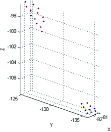
The result of the efficient point set extraction near the line of sight (Color figure online)

2.4 Surface Fitting Efficient Point Set
According to the interpretation for the intersection of the line of sight and the point cloud, the intersection of the line of sight and the object was actually the intersection of the line of sight and the curved surface expressed by the efficient point set near the line of sight.
The setting of the threshold \( {\text{r}} \) was generally smaller during the extracting the point cloud near to the line of sight. At the same time, according to the demand of the rapid response in the user interaction, the least square plain fitting to the efficient point set was adopted to the express the local surface of object in the method. The method was as follows.
The equations of plane was set as \( z = - Ax - By + D \). Substituted all the points in the efficient point set into the equation, the least square error formula could be obtained and shown as the formula (7).
Due to the \( \nabla E = 0 \), the least square solution of the \( A,B,D \) could be obtained and shown as the formula (8).
In the formula, \( {\text{n}} \) expressed the number of the point sets. \( x_{i} ,y_{i} ,z_{i} \) was the coordinate value of the point \( i \). The least square estimation of the local surface could be obtained through the solving of the equation set. For the convenience of the calculating of the intersection of the line of sight and the fitting plane, the vector V was defined as \( v = \left( {A,B,1} \right) \), the vector P was defined as \( P = \left( {x,y,z} \right) \). Thus, the plane equation could be expressed as the vector expression and shown in the formula (9).
2.5 Calculating the Intersection Between the Line of Sight and the Object Surface
Contact the formula (9) and the formula (3), the parameter t of the point of intersection between the line of sight of users and the fitting local surface of the object could be determined and shown as the formula (10). After that, as shown in Fig. 5, the intersection point could then be found.

The intersection point of the line of sight and the object
3 Result and Analysis
Using the point cloud data of the wheat plant collected in Henan agricultural university science park from 2012 to 2013 as the experimental material, adopting the C++ language, with the help of the software library such as OpenGL, PCL [16] and so on, the interactive wheat plant surface pastry coordinates calculating algorithm was realized at the Ubuntu12.04 system environment in the research and shown in Fig. 6. As shown in Table 1, using the mark function of the supporting tools software of the FastSCAN 3D digital scanner, the mapping from the screen pixels to the object surface coordinates was verified. The results showed that the error of the proposed mapping method in this paper was less than 2.1 mm compared with the FastSCAN and had good accuracy. Because there was no direct intersection between the line of sight and the point cloud in this study, the error of the interactive selection of the points was mainly produced by different user perspective. As shown in Tables 2 and 3, this study conducted the comparison validation with the 10°, 20° and the 0° viewing angle respectively. The results showed that the error of the method was less than 1.8 mm in the normal range of angle and had good accuracy.

Interactive measurement of point
4 Conclusion
Using the scattered three-dimensional point cloud data of the wheat plant as the research object, through the procedure including “Solving the user sight equation passing the given screen pixel point–Screening the point cloud near the line of sight– Extracting efficient point set in the point cloud near the line of sight– Surface fitting efficient point set–Calculating the intersection between the line of sight and the object surface”, the mapping from the screen pixel point to the object surface coordinate point was formed. It could map the window coordinate of the user’s mouse to the object surface which expressed by the point cloud and realize the calculation for the wheat plant surface point coordinate. T This method had certain universality and could to provide technical reference for the construction of the interactive plant to geometry measurement based on point cloud data.
References
Boissionnat, J.D.: Geometric structures for three-dimensional shape representation. ACM Trans. Graph. 3(4), 266–286 (1984)
Dey, T.K., Goswami, S.: Tight cocone: a watertight surface reconstructor. J. Comput. Inf. Sc. Eng. 3(4), 302–307 (2003)
Dey, T.K., Goswami, S.: Provable surface reconstruction from noisy samples. Comput. Geom. 25(1), 124–141 (2005)
Yinxi, G., Cheng, H., Zhongke, F., Wenzhao, L., Fei, Y.: Amended Delaunay algorithm for single tree factor extraction using 3-d crown modeling. Trans. Chin. Soc. Agric. Mach. China 44(2), 192–199 (2013)
He, C., Feng, Z., Yuan, J., Wang, J., Dong, Z., Gong, Y.: Three-dimensional volume measurement of trees based on digital elevation model. Trans. Chin. Soc. Agric. Mach. China 28(8), 195–199 (2012)
Paulus, S., Dupuis, J., Mahlein, A.K., Kuhlmann, H.: Surface feature based classification of plant organs from 3D laserscanned point clouds for plant phenotyping. BMC Bioinform. 14, 238 (2013)
Shenglian, L.U., Xinyu, G.U.O., Changfeng, L.I.: Research on techniques for accurate modeling and rendering 3d plant leaf. J. Image Graph. China 14(4), 731–737 (2009)
Zhao, Y., Wen, W., Guo, X., Xiao, B., Lu, S., Sun, Z.: Midvein extraction for 3-d corn leaf model based on parameterization. Trans. Chin. Soc. Agric. Mach. China 42(4), 183–187 (2012)
Takahashi, S.T.: Comperhensible rendering of 3-D shapes. Comput. Graph. 24(4), 197–206 (1990)
Dong, Z., Mingyong, P.: Algorithm for extracting sharp features from point cloud models. Trans. Chin. Soc. Agric. Mach. China 42(11), 222–227 (2011)
Qian, L., Geng, G., Zhou, M., Zhao, L., Li, J.: Algorithm for feature line extraction based on 3D point cloud model. Appl. Res. Comput. China 30(3), 933–937 (2013)
Birant, D., Kut, A.: ST-DBSCAN. An algorithm for clustering spatial-temp oral data. Data & Knowl. Eng. 60(1), 208–221 (2007)
Elsner, G.: A new sequential cluster algorithm for optical lens design. J. Optim. Theory Appl. 59(2), 165–172 (1988)
Hinneburg, A., Gabriel, H.-H.: DENCLUE 2.0: fast clustering based on kernel density estimation. In: R. Berthold, M., Shawe-Taylor, J., Lavrač, N. (eds.) IDA 2007. LNCS, vol. 4723, pp. 70–80. Springer, Heidelberg (2007). doi:10.1007/978-3-540-74825-0_7
Zhou, W., Feng, X., Sun, G.: Classification based on feature extraction from cluster of wavelet coefficients. J. Comput. Res. Develop. 1–12, 982–988 (2001)
Point Cloud Library (2014). http://www.pclcn.org/study/shownews.php?lang=cn&id=29
Acknowledgements
This study has been funded by China National 863 Plans Projects (Contract Number: 2008AA10Z220) and key scientific and technological project of Henan Province (Contract Number: 082102140004).
Author information
Authors and Affiliations
Corresponding author
Editor information
Editors and Affiliations
Rights and permissions
Copyright information
© 2016 IFIP International Federation for Information Processing
About this paper
Cite this paper
Xi, L., Zheng, G., Ren, Y., Ma, X. (2016). An Algorithm for the Interactive Calculating of Wheat Plant Surface Point Coordinates Based on Point Cloud Model. In: Li, D., Li, Z. (eds) Computer and Computing Technologies in Agriculture IX. CCTA 2015. IFIP Advances in Information and Communication Technology, vol 478. Springer, Cham. https://doi.org/10.1007/978-3-319-48357-3_6
Download citation
DOI: https://doi.org/10.1007/978-3-319-48357-3_6
Published:
Publisher Name: Springer, Cham
Print ISBN: 978-3-319-48356-6
Online ISBN: 978-3-319-48357-3
eBook Packages: Computer ScienceComputer Science (R0)