Geostatistics for Variable Geometry Veins

Abstract

This paper presents the idea of applying a modified “moving trihedral” borrowed from the abstract Theory of the Geometry of Riemann, allowing us to model the random functions L²(Ω, σ, P) of geostatistics, in a special 2-D plane within such trihedral, a feature not available in any software existing in the market. Thus, from working in the R² space in that trihedral plane, we obtain our results in the R³ physical space, in which we can then derive the desired linear or nonlinear geostatistical results. The method presented here therefore can be considered akin to a kind of spatially adaptative geostatistics. And so, among other applications of this method, it becomes possible to apply geostatistics simply, without the need for a detailed, three-dimensional geological model of the mineralization, defining instead its contours in a simple plane, a feature very useful when modelling irregular veins.

Appendices

Annex 1: Frame Theory Riemannian Manifold

1.1 Differentiable Manifolds

A differentiable manifold is a type of manifold (In mathematics, a manifold is a topological space that locally resembles Euclidean space each point. More precisely, each point of an n-dimensional manifold has a neighbourhood that is homeomorphic to the Euclidean space of dimension n.) that is locally similar enough to a linear space to allow one to do calculus. Any manifold can be described by a collection of charts, also known as an atlas. One may then apply ideas from calculus while working within the individual charts, since each chart lies within a linear space to which the usual rules of calculus apply. If the charts are suitably compatible (namely, the transition from one chart to another is differentiable), then computations done in one chart are valid in any other differentiable chart (Warner 1983).

In other words a complex spatial feature can be represented by local, well-behaved, simple patches, possibly of lower dimensions, and under certain mathematical conditions (i.e. differentiability); they accurately describe the entirety of that feature continuously in its space of origin.

Mathematical Definition

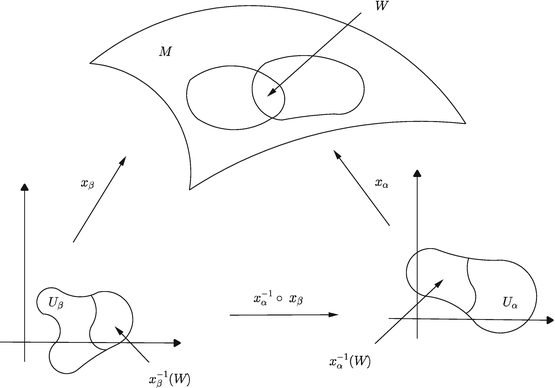
A differentiable manifold of dimension n is a set M and a family of bijective mappings

$$ {x}_{\alpha}:{U}_{\alpha}\subset {\mathrm{\mathbb{R}}}^n\to M $$

of open sets U _α of ℝⁿ into M such that

• 1. ${\cup}_{\alpha}{x}_{\alpha}\left({U}_{\alpha}\right)= M$.

• 2. For any pair α, β with $W={x}_{\alpha}\left({U}_{\alpha}\right)\cap {x}_{\beta}\left({U}_{\beta}\right)\ne \phi$, the sets ${x}_{\alpha}^{-1}(W)$ and ${x}_{\beta}^{-1}(W)$ are open in ℝⁿ and the mappings ${x}_{\alpha}^{-1}{\mathrm{ox}}_{\beta}$ are differentiable (see Fig. 1).

• 3. The family $\left\{\left({\cup}_{\alpha},{x}_{\alpha}\right)\right\}$ is maximal relative to the conditions (1) and (2).

  

1.2 Tangent Space on Manifolds

Definition

Let M be a differentiable manifold, and let p be a point of M. A linear map $v:{C}^{\infty }(M)\to \mathrm{\mathbb{R}}$ is called a derivation at p if it satisfies the Leibniz rule:

$$ v\left(\mathrm{fg}\right)= f(p) v g+ g(p) v f;\forall f, g\in {C}^{\infty }(M) $$

The set of all derivations of ${C}^{\infty }(M)$ at p, denoted by T _p M is called a tangent space to M at p. An element of T _p M is called a tangent vector at p.

A Riemannian metric on a differentiable manifold M is a correspondence which associates to each point p of M, an inner product 〈, 〉 _p on the tangent space T _p M, which varies differentiably; this metric is also called the metric tensor.

A differentiable manifold with a given Riemannian metric will be called a Riemannian manifold (Lee JM 2013; Do Carmo 1976).

Annex 2: Applying Methodology in Euclidean Space ℝ³

An example of Riemannian manifold in the Euclidean space ℝ³ is a surface of dimension 2 with the usual metric ℝ³ and the tangent space here is a plane.

2.1 Regular Surface

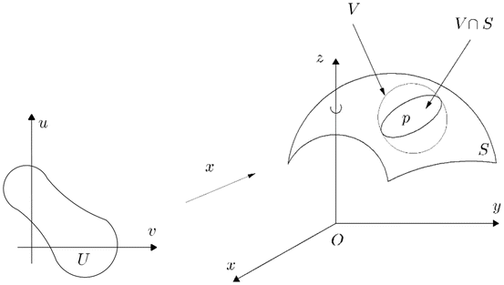
A subset $S\subset {\mathrm{\mathbb{R}}}^3$ is a regular surface if, for each $p\in S$, there exists a neighbourhood Vin ℝ³ and a map $x: U\to V\cap S$ of an open set $U\subset {\mathrm{\mathbb{R}}}^2$ onto $V\cap S\subset {\mathrm{\mathbb{R}}}^3$ such that (see Fig. 1):

• 1. x is differentiable.

• 2. x is homeomorphism.

• 3. $\forall q\in U,{\mathrm{dx}}_q:{\mathrm{\mathbb{R}}}^2\to {\mathrm{\mathbb{R}}}^3$ is one-to-one.

  

2.2 The Tangent Plane

Definition

Let $v\in {\mathrm{\mathbb{R}}}^3$ be a tangent vector to S at a point $p\in S$; it exists a differentiable parametrized curve $\left.\alpha :\right]-\varepsilon, \varepsilon \left[\to S\right.$ with ${\alpha}^{\prime }(0)= v$ and $\alpha (0)= p$.

The set of all tangent vectors to S at p will be called the tangent plane to p and will be denoted by T _p S (Do Carmo 1976) (see Fig. 2).

$$ {T}_p S=\left\{ v\in {\mathrm{\mathbb{R}}}^3; v\ \mathrm{is}\ \mathrm{tangent}\ \mathrm{vector}\ \mathrm{to}\ S\ \mathrm{at}\ p\in S\right\} $$

2.3 Proposed Trihedron

Now let us build a trihedron, from a point on the surface and a tangent vector to the surface at that point; this construction is a different wing of the trihedron Frenet-Serret; in very specific cases of surface geometry, these may coincide.

Let $S\subset {\mathrm{\mathbb{R}}}^3$ a regular surface, parametrization (x,U) at point $p\in S$ and a regular parametrized curve $\left.\alpha :\right]-\varepsilon, \varepsilon \left[\to {\mathrm{\mathbb{R}}}^3\right.$ content in S such that ${\alpha}^{\prime }(0)= v$ and $\alpha (0)= p$, clearly $v\in {T}_p S$.

On the T _p S tangent plane, rotate the vector v angle π/2 in a sense counterclockwise forming a basis for the tangent plane T _p S (see figure). We now vector cross product $w= v\times u$ and form the proposed trihedron (see Fig. 3).