A Shape-Based Approach for Salient Object Detection Using Deep Learning

Abstract

Salient object detection is a key step in many image analysis tasks as it not only identifies relevant parts of a visual scene but may also reduce computational complexity by filtering out irrelevant segments of the scene. In this paper, we propose a novel salient object detection method that combines a shape prediction driven by a convolutional neural network with the mid and low-region preserving image information. Our model learns a shape of a salient object using a CNN model for a target region and estimates the full but coarse saliency map of the target image. The map is then refined using image specific low-to-mid level information. Experimental results show that the proposed method outperforms previous state-of-the-arts methods in salient object detection.

1 Introduction

Visual saliency is one of the fundamental problems in computer vision. It aims to automatically identify the most important and salient regions/objects in an image. The saliency detection slightly differs from general semantic image segmentation in that it seeks to elucidate salient foreground structures from otherwise “irrelevant” background whereas semantic segmentation algorithms partition an image into regions of coherent properties [4]. As it can also reduce computational complexity by focusing on the interest regions, saliency detection has recently received attention in the context of many computer vision problems including object detection, image segmentation and classification.

Many recent works have focused on the specific task of detecting salient objects [4, 8, 9, 11, 19, 20, 27, 29, 30, 33, 35, 37]. The central task there is to estimate a saliency score of an image patch/superpixel using visual features extracted on the patch/superpixel. To this end, classifiers (or regressors) are trained on the extracted features to determine the saliency score [8, 11, 27, 35].

For training the classifiers, a single binary label is traditionally assigned to the patch based on the normalized overlap rate between the patch and its ground truth salient map [27, 35]. The overlap rate ranges from 0 to 1; 0 represents no salient region in the patch, and 1 means that the patch is fully contained in the salient region. Then the binary label is obtained by thresholding the overlap rate.

The binary classification-based approaches are limited in that they ignore the shape of the salient region in the patch by assigning a single (univariate) output value to an input (patch or superpixel). Moreover, the patches whose overlap rates are around 0.5 are often ignored to prevent the classifiers from being confused. This results in two critical drawbacks: (1) the valuable data is excluded from the training process and (2) the geometric precision of saliency, in particular for overlaps around 0.5, will be significantly degraded.

To overcome the aforementioned limitations of the binary classification approach, we propose a new method that takes explicit shape of the salient region into consideration. In the proposed method, we model the prediction of the shape of the salient region as a multi-label classification problem. An image patch is assigned to a binary $m \times n$ map so that the map closely resembles the ground truth salient map of the image patch. Therefore, the proposed method can be considered as a structured output prediction approach by considering correlations of saliency “pixels” in the output. This results in more accurate shape-preserving saliency prediction compared to the binary all-salient or all-non-salient traditional representation. Our goal is to learn the image representation to accurately predict the binary map.

Fig. 1.

The overview of the proposed saliency detection framework. First, we generate region proposals from an input image. The regions’ saliency map is then assessed by a specifically structured and trained CNN. Finally, we refine the saliency map using a hierarchical segmentation.

An overview of our salient object detection approach is depicted in Fig. 1. Our specific computational model uses a convolutional neural network (CNN) as a multi-label classifier not only because of CNN’s strong empirical performance in many vision problems but also because they leverage and directly encode spatial image content. The spatial information is one of the important properties for our task because we want to discover locations and shapes of the salient regions. Unlike the binary classification approaches, the proposed method does not ignore the patches whose overlap rates are around 0.5. Instead, it uses all the patches by extending the binary representation into the $m \times n$ binary map and learns rich representations of the salient regions. To achieve this goal, we propose a new CNN framework to capture not only the local context of a local region of an image but also address the global information of the image.

Despite this geometrically more accurate representation, the predicted saliency map using the CNN may be insufficient to accurately delineate salient shape boundaries as the CNN does not explicitly take the global image context, such as the object placement or image boundaries, into consideration. For instance, as illustrated in Fig. 1, the saliency map detected by the CNN model largely agree with the ground truth maps. However, the boundaries are excessively blurred. Therefore, we combine the output of the CNN with the target-driven hierarchical image segmentation. This combination eliminates over-smoothing and results in improved salient object boundaries.

In summary, this paper makes the following key contributions: (1) we propose a novel method that accurately estimates the shape of the salient region by treating the prediction problem as a structured multi-label classification task, (2) a new CNN architecture that addresses both global and local context of an image is proposed, (3) by effectively combining the deep learning method and the hierarchical segmentation, the proposed method assures accurate delineation of saliency boundaries through the use of image context. As a result it outperforms previous approaches and shows the state-of-the-art performance in saliency detection.

2 Related Work

Over the recent years, the convolutional neural network (CNN) model has demonstrated significant gains in performance for many tasks in computer vision, where sufficient training data is available. Aided by computational speedups resulting from highly-parallelized and efficient GPU implementations, tasks such as object detection, segmentation, and recognition [6, 7, 14, 31, 32, 34] have seen significant gains in performance. In this paper, we use the CNN framework for the saliency detection as a multi-class classifier. Instead of training the CNN from scratch, we train our model in a similar manner of fine-tuning a pre-trained convolutional network for our purpose so that the proposed method can adapt the knowledge gained on a large dataset to the current task. The fine-tuning methods are known to successfully perform in a variety of problems in computer vision [18, 22, 34, 36].

Salient object detection has attracted key interest in many computer vision applications. Comprehensive surveys of salient object detection and visual attention modeling can be found in [3, 4]. A seminal work, Itti et al. proposed bottom-up visual saliency using biologically inspired center-surround differences across multi-scale image features [9]. An alternative approach to use local contrast using a fuzzy growth model is proposed in [19]. In [30], a bottom-up method to detect salient regions using graph-based manifold raking was proposed. Jiang et al. [11] proposed a method to integrate discriminative regional features to compute the saliency scores. Image boundary prior, which assumes that most image boundary regions are background, has been shown to be effective for object saliency detection [25, 30, 33].

Salient object detection methods using the deep learning methods have been recently proposed [8, 27, 35, 37]. Wang et al. [27] proposed to use two convolutional neural networks. One of them is used to learn local patch features to estimate a saliency value of each pixel and the other to incorporate global features such as global contrast and geometric information. Hierarchy-associated features to represent the global context of the salient object were proposed in [37]. Zhao et al. [35] proposed a CNN architecture that considers both global-context and local context saliency. Our method is different from the previous approaches in that we estimate a shape of a salient object in a region instead of determining the binary saliency score on each pixel or region.

Several other approaches have been proposed to use shape dictionaries for segmentation [13, 16, 24] to address the shape of the object beyond the binary representation. In those methods, the shape dictionaries, whose words represented pre-defined shapes, constructed by clustering image patches or descriptors. During prediction, the word closest to the input image in the shape dictionaries is assigned as the prediction result. Unlike the traditional binary representation, these models can attempt to preserve the underlying object/boundary shape. The shape dictionary-based approaches, however, have limitations. First, they predict the shape of the object in the scope of the pre-defined dictionaries. Therefore, how to construct the shape dictionaries (e.g., the number of the clusters) must be carefully examined to assure accurate generalized performance and boundary accuracy. Second, by treating the problem as a multi-class (basis shape) classification, they inadvertently impose the 0–1 loss among classes which does not reflect difference degrees of basis shape similarities. To address this problem, we use the CNN as a multi-label classifier, which will lead to the Hamming, shape-sensitive, loss required for fine boundary delineation.

3 Proposed Method

In this section, we first define the patch-based representation of saliency, which will be the key representation used in our predictive model. Then we describe our architecture of a convolutional neural network (CNN) for salient object detection and how to train it. Next we explain the proposed framework to predict a saliency map using the trained CNN model. Lastly, we describe the refinement of the saliency map using the mid and low-level information such as hierarchical segmentations.

Fig. 2.

Visualization of region proposals and their encoded binary saliency map representations. We generate region proposals, $\{X_1, \ldots , X_6\}$, on image I. Then we map them to encoded binary saliency maps of size $m \times n$, $\{Y_1, \ldots , Y_6\}$ by affine map $f_I(X_k)$.

3.1 Saliency Representation

In the previous binary-based or shape dictionary-based approaches for the salient object detection, an image patch associated with a binary value (e.g., presence or absence of the object in the patch) or a label (representing the dictionary shape closest in appearance to the saliency map). Instead, we directly represent the saliency map in the patch using an $m\times n$ binary map, as illustrated in Fig. 2. Note that the resolution of this map need not to be the same as the resolution of the original saliency map, instead it typically represents a coarse approximation. Our goal is to predict this binary map by treating the prediction problem as a multi-label classification.

Image-based saliency could, in principle, be encoded based on saliency of a set of dense, overlapping, patches that fully span the image. However, this representation is typically highly (computationally) inefficient. Instead, we define image saliency based solely on the saliency of representative image regions. In particular, we use selective search [26] to extract category-independent region proposals as it is fast and showed successful performance in the object detection tasks [1, 7].

Formally, for image I we generate K region proposals, $\{X_1, X_2, \ldots , X_K\}$ by a region proposal method (selective search), where $X_k$ is the k-th representative region of size $h_k \times w_k$ centered at position $(s_k, t_k)$. Each $X_k$ is mapped to $Y_k$ of size $m \times n$, the encoded binary saliency map of region $X_k$, $Y_k = f_I(X_k)$, where $f_I(\cdot )$ is the affine map from $X_k$ to $Y_k$. We aim at predicting all entries of $Y_k$ as the multi-label classification.

Figure 2 depicts sample region proposals and corresponding encoded binary saliency maps. We can observe that our saliency representation accurately preserves the shape information of the objects.

Fig. 3.

The architecture of our shape-based saliency detection model. The CNN contains two branches: the top branch processes a fine-level image patch to handle local-context while the bottom addresses global-context contained in a coarse-level image patch. Two branches are combined to fully connected layer fc8. We adopt AlexNet [14] for two branches up to fc7. We tie weights between two branches, denoted by dashed arrows, so that the same fc-level feature embedding functions is used for two input patches. Then joint relationship is estimated at fc8.

3.2 Convolutional Neural Networks for Shape Prediction

In this section, we explain our shape-based saliency detection framework (SSD) using convolutional neural networks (CNN) for salient object detection. We aim at training the CNN for the multi-label classification so that it will be able to predict the salient shape of the object accurately.

Figure 3 shows the architecture of the CNN designed for our purpose. The CNN contains two branches, one for fine representation (top) and the other for coarse representation (bottom). For the fine representation, we feed region proposal $X^f$ of size $h\times w$ centered at position (s, t) to the CNN to predict the saliency. However, an isolated image patch may be insufficient to determine the saliency as it contains only the local information, excluding the important regional context. To include contextual information from the neighborhood of $X^f$ to the CNN, we extract a larger image patch $X^c$ so that $X^c$ has the same center position (s, t) with size $\alpha h\times \alpha w$ where $\alpha > 1$ is a magnification factor. In this way, the CNN leverages the local content within $X^f$ and combines it with the regional context in $X^c$.

For the implementation, we use a pair of AlexNet-like architectures [14] each of which has the same architecture as AlextNet up to fc7 as illustrated in Fig. 3. The fine representation branch processes $X^f$ to address the local information while the coarse representation branch exploits the global context contained in $X^c$. We tie weights between two branches up to fc7 so that the same fc-level feature embedding function is used for both coarse and fine patches. Then two $\texttt {fc7}$s in both branches are concatenated and fully connected to fc8 where joint relationship between $X^f$ and $X^c$ is estimated. We use the sigmoid layer for pred so that each entry in the output has a real value in the range of 0 and 1. We train the proposed architecture in an end-to-end manner.

Training. We can train AlexNet by minimizing a negative log-likelihood cost function as follows:

$$\begin{aligned} L = -\frac{1}{N} \sum _{i=1}^{N} \sum _{l=1}^{L}\delta (y_i = l) \cdot \log \left( \hat{p}_{l}(x_i)\right) , \end{aligned}$$

(1)

where N and L are the numbers of the training samples and the labels, respectively, $x_i$ the i-th input, $y_i \in (1, 2, \ldots , L)$ the ground truth label for $x_i$, $\hat{p}_{l}(x_i)$ the prediction probability of $x_i$ for the l-th label, and $\delta (\cdot )$ the indicator function.

Our goal is to predict entries of a $m \times n$ patch under the multi-label classification. To achieve this, we use the sigmoid cross entropy loss function to optimize the proposed CNN as follows:

$$\begin{aligned} L = -\frac{1}{N}\sum _{i=1}^{N}\sum _{l=1}^{mn}\bigg [Y_i(l) \log \left( \hat{p}_l(X^f_i, X^c_i)\right) + (1-Y_i(i)) \log \left( 1-\hat{p}_l(X^f_i, X^c_i)\right) \bigg ], \end{aligned}$$

(2)

where N is the number of training samples, $Y_i(l)$ the l-th binary value of i-th encoded saliency map $Y_i$, and $\hat{p}_l(X^f_i, X^c_i)$ the prediction probability of our CNN taking $X^f_i$ and $X^c_i$ as inputs. We can train our convolutional neural network by minimizing the loss function in (2).

Prediction. To predict a saliency map for a given image, we first generate region proposals using selective search to obtain category-free object regions on the image. The region proposal method reduces the search space by allowing us to focus on the interest regions where objects are likely to appear. Therefore, we can reduce the number of the CNN evaluations instead of exhaustively running the CNN on the entire image.

For a given image $I^{h \times w}$, we generate region proposals $\{X^f_1, \ldots , X^f_K\}$ by selective search, and corresponding $\{X^c_1,\ldots , X^c_K\}$ as explained. We then run the CNN by feeding $X^f_k$ and $X^c_k$ as inputs and predict a salient object shape, $p_k$. Next, we perform the affine transformation to map $p_k^{m\times n}$ back to the position $(s_k, y_k)$ with size $(h_k, w_k)$, pad zeros outside the transformed area to obtain a saliency prediction map $P_k^{h \times w}$.

The final saliency map for the whole image is the average of the prediction results, $\{P_1, P_2, \ldots , P_K\}$. Let $C^{h \times w}$ be a matrix for normalization where C(l) denotes the number of the region proposals containing the l-th entry (pixel). Then the saliency map S for input image I is computed as follows:

$$\begin{aligned} S(l) = \left\{ \begin{array}{ll}0 &{} \qquad \text{ if } C(l) = 0\\ \frac{\sum _{k=1}^{K} P_k(l)}{C(l)}&{}\qquad \text{ if } C(l) > 0\end{array}\right. , \end{aligned}$$

(3)

where l denotes the l-th entry.

3.3 Refinement of Saliency Maps Using Hierarchical Segmentations

In this section, we explain our shape-based saliency detection using the hierarchical segmentation (SSD-HS) method for refinement. The CNN-based prediction proposed above may not consider spatial consistency or boundaries of objects in the image as it processes the region proposals independently. As a results, the predicted salient maps usually show fuzzy object boundaries as depicted in Fig. 4 (third column, SSD).

To overcome this limitation, we refine the predicted saliency map using the target image-specific segmentation proposals. The main role of the segmentation is to provide informative boundary cues so that we can find pixel-wise accurate candidates of the objects as well as maintain the global spatial consistency.

To achieve this, we generate a set of L-level hierarchical segmentation proposals $M = \{M_1, M_2, \ldots , M_L\}$ where $M_1$ is the finest segmentation with the largest number of segmented regions and $M_L$ is the coarsest with the smallest number of regions for image I. Note that $M_l$ is computed by merging the regions in $M_{l-1}$. In this way, we build a hierarchy in the set of L-level segmentations. We use an ultrametric contour map (UCM) generated by the gPb (globalized probability of boundary based contour detection) [2] to build the hierarchical segmentation for our purpose. The UCM contains a set of real valued contours to reflect the contrast between neighboring regions. We generate the hierarchical segmentation maps by thresholding the UCM with L different values.

Let $R_l(i)$ be the i-th region (superpixel) on the l-th level segmentation $M_l$. We define the saliency score in $R_l(i)$, $M_l(i)$, as the expected saliency prediction score computed by the CNN in that region as follows:

$$\begin{aligned} M_l(i) = \frac{1}{|R_l(i)|} \sum _{p\in R_l(i)} S(p), \end{aligned}$$

(4)

where p is a pixel in region $R_l(i)$, S(p) the predicted saliency value at pixel p, and $|R_l(i)|$ the number of the pixels in $R_l(i)$. Then we compute the refined saliency map for the l-th level, $S_l$, by assigning $M_l(i)$ to all pixels in $R_l(i)$:

$$\begin{aligned} S_l(p) = M_l(i), \qquad p \in R_l(i). \end{aligned}$$

(5)

In this way, we have L refined saliency maps, $\{S_1, S_2, \ldots , S_L\}$ for image I.

Figure 4 shows the refined multi-level saliency maps generated by (5). In the finer level, boundaries of the objects are preserved while there are many artifacts in the background. As we move toward the coarser level, those artifacts become weaker. On the other hand, we lose the accurate object boundaries. Therefore, we need to combine the multi-level saliency maps to both preserve accurate delineation of saliency boundaries and reduce the artifacts.

A problem of fusing the multi-level saliency maps to generate a final output has been previously discussed including approaches to use the conditional random field (CRF) [17] or the regression method [11]. In this paper, we use a least-square estimator as it is fast to compute and results in strong performance. Formally, we formulate the following optimization problem to find weights $\mathbf {w} = \{w_1, \ldots , w_l\}$ to linearly combine the multi-level saliency maps:

$$\begin{aligned} \arg \min _{\mathbf {w}}&\sum _{I \in \mathbf {V}} \left\| Y^I - \sum _{l=1}^L w_l S^I_l\right\| _F^2, \\ \text{ s.t. }&\sum _{l=1}^L w_l = 1, \qquad w_l \ge 0 \quad (l=1, 2, \ldots , L) \nonumber \end{aligned}$$

(6)

where $\mathbf {V}$ denotes the validation set, and $Y^I$ the ground truth saliency map for image I. The final saliency map is computed as the weighted linear sum of the multi-level saliency maps, $\sum _{l=1}^L w_l S_l$. As desired, the fused map shows accurate boundaries and little artifacts as depicted in Fig. 4 (last column, SSD-HS).

Fig. 4.

Visualization of multi-level saliency maps using the hierarchical segmentations. SSD, detected by the CNN, initially shows fuzzy boundaries and artifacts. By aggregating saliency maps from $S_1$ (finest) to $S_8$ (coarsest), SSD-HS successfully delineates accurate object boundaries and smooths out the artifacts.

4 Experimental Results

In this section, we explain our experimental settings including the datasets we used in the paper and the CNN settings. We then examine the performance of our saliency representation and compare it to other baseline methods. Next, we show the saliency prediction results using the proposed method and compare to state-of-the-art methods in saliency detection. Lastly, we analyze the multi-context representation used in our CNN architecture.

4.1 Experimental Settings

Benchmark Datasets. To evaluate the performance of the proposed method, we use several datasets that are widely used for saliency detection including MSRA-5000 [17], SOD [21, 28], ECSSD [29] and PASCAL-S [15]. Each dataset provides pixel-wise ground truth annotation for the salient objects. MSRA-5000 is the largest dataset, consisting of 5000 images that cover a large variety of image contents including natural scenes, animals, indoor, outdoor and so on. SOD is a collection of salient object boundaries based on Berkeley Segmentation Dataset. SOD is challenging as it has 300 images with multiple objects. ECSSD includes many semantically meaningful but structurally complex images in 1000 images. PASCAL-S dataset contains 850 natural images with complex objects and backgrounds.

Evaluation Criteria. We evaluate the performance of the proposed method using the precision-recall (PR) curve and the F-measure. For the PR curve, we increase the threshold from 0 to 255 and measure the precision and recall of a saliency map. We compute the maximal F-measure of the average precision-recall curve as in [4]. The F-measure is a harmonic mean of precision and recall defined as:

$$\begin{aligned} F_\beta = \frac{(1+\beta ^2)\cdot (P \times R) }{\beta ^2 \cdot P + R}, \end{aligned}$$

(7)

where P and R are precision and recall, respectively. We set $\beta ^2$ to 0.3 because we want to emphasize the precision more than the recall [4, 27].

Experimental Settings and Training CNN. We split the MSRA-5000 dataset into training, validation and test sets as suggested in [11]. We do not use other datasets during training because not only they do not have as many images as MSRA-5000 does but also we want to examine how well the proposed model can be adapted to different datasets without overfitting. We use selective search to generate patches on the training set and randomly select 100,000 patches to train our CNN model.

We use the open-source package Caffe [10] to implement our CNN model. In our implementation, we initialized the weights of our network by adopting those of AlexNet trained on ImageNet [5] where possible in a fine-tunning manner instead of training the CNN from scratch. As our CNN takes a pair of two images whose sizes are $227\times 227$, we resize the input images by the bilinear interpolation before we feed them to the CNN.

We set $\alpha = 2$ such that $X^c \in \mathcal {R} ^{2m \times 2n}$ includes the neighborhood information of $X^f \in \mathcal {R} ^{m \times n}$. We use a square encoded binary saliency map, i.e., $m=n$. For the hierarchical segmentation maps, we empirically set the number of the maps L to 16 by thresholding the UCM map from 0.2 to 0.95 quantiles with a step size 0.05.

Fig. 5.

Visualization of selected shape classes.

4.2 Experimental Results

Evaluation on Various Schemes for Saliency Representation. To determine the optimal size of the encoded saliency map, we perform experiments with various sizes, $m \in \{8, 16, 24, 32\}$. The experimental results are shown in Table 1. If m is too small, it may be insufficient to represent accurate shapes because the affine map loses much information. On the other hand, as we increase m, the complexity of the encoded map increases. Consequently, SSD ($16 \times 16$) shows the best performance so that we set $m=16$ hereafter.

Experimental results with two additional $\alpha \in \{1.5, 3\}$ are also shown in Table 1. $\alpha =3$ shows worse performance than $\alpha =2$ (i.e., SSD $16 \times 16$) because the coarse patch may be too large, losing the information of the object shape. On the other hand, if the coarse patch looks at a smaller region, i.e., $\alpha =1.5$, it may fail to consider the global context, resulting in worse performance than $\alpha =2$.

To set baseline methods, we adopt binary representation-based and shape dictionary-based approaches, and fully convolutional networks as follows:

• Binary representation (BIN)

  We use the traditional binary representation as a baseline method. In this approach, a region proposal is mapped to a binary value by thresholding the normalized overlap rate between the region and its ground truth map. Note that BIN can be easily implemented by setting $m=n=1$ in our framework.

  Table 1. F-measure scores for baseline and proposed methods on four benchmark datasets. Red and blue colors denote the best and the second best results, respectively.

  Fig. 6.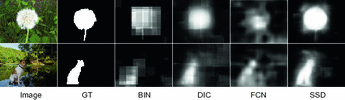

  

  Saliency maps generated by baseline and proposed methods. GT: ground truth. BIN: binary representation. DIC: dictionary-based representation. FCN: fully convolutional networks. SSD: our shape-based salient detection method.

• Dictionary-based representation (DIC)

  We encode the saliency map using pre-defined shape classes as in [13, 16, 24]. For this purpose, we cluster normalized region proposals to construct a dictionary with D shape classes, $\{V_1, V_2, \ldots , V_D\}$. Sample shape classes are depicted in Fig. 5. Then we train a $\text{ CNN }^{\text{ DIC }}$ as a multi-class classifier to predict the shape class closest to the region proposal. For region proposal $X_k$, we compute its local saliency map as an expected shape over prediction of the $\text{ CNN }^{\text{ DIC }}$:

  $$\begin{aligned} P_k^{\text{ DIC }} = \sum _{d=1}^D V_d \cdot \text{ CNN }_d^{\text{ DIC }}(X_k), \end{aligned}$$

  (8)

  where $\text{ CNN }_d^{\text{ DIC }}(X_k)$ is the prediction probability of $X_k$ for shape class d. Then we can compute the final saliency map by replacing $P_k$ with $P_k^{\text{ DIC }}$ in (3). We set D to 64 as in [13].

• Fully convolutional network (FCN)

  FCN allows us to predict a full sized saliency map by introducing deconvolution layers [18]. FCN is similar to our approach in that it directly estimates the shape of the salient object. However, FCN takes the entire image into consideration while our method focuses on the salient object areas by employing the region proposal method. For the implementation, we fine-tune a pre-trained model provided by the authors of [18]. We set the number of classes to two (0 for a background pixel, 1 for a salient object pixel). We normalize the output of FCN using the softmax function for our purpose.

Experimental results in Table 1 confirm that the proposed shape-based approach outperforms the other baseline methods. For the qualitative analysis, we depict sample saliency maps in Fig. 6. BIN performs the worst because it ignores the shape information and therefore fails to delineate accurate object boundaries. FCN computes the saliency values on the entire image while the proposed SSD focuses on the object regions. Therefore, SSD can highlight the salient regions without being distracted by the background areas, resulting in better performance than FCN as shown in Fig. 6. DIC performs worse than the proposed method as it represents the object’s shape as a combination of the pre-defined shape classes while the proposed method can estimate an arbitrary shape. As a result, DIC results in coarse saliency maps while our SSD detects accurate silhouettes of objects as illustrated in Fig. 6.

Fig. 7.

Saliency maps generated by different methods for comparison including SF [23], HDCT [12], PCA [20] HS [29], MR [30], DRFI [11], LEGS [27], MB [33], DMC [35], and MDF [8]. GT denotes ground truth. SSD and SSD-HS are the proposed methods.

Comparison to Previous Methods. To evaluate the performance of the proposed method, we compare our method to 10 state-of-the-art methods in salient object detection including SF [23], HDCT [12], PCA [20] HS [29], MR [30], DRFI [11], LEGS [27], MB [33], DMC [35], and MDF [8]. Figure 8 shows the performance evaluation results in terms of the Precision-Recall curve (PR-curve). Our SSD-HS shows the best performance among the other methods over the four datasets as shown in Fig. 8. The performance of SSD is also comparable to the other methods in all the benchmark datasets. These results confirm the importance of the shape prediction-based approach for salient object detection. The F-measure scores over the four benchmark datasets also verify that the proposed method outperforms the others as shown in Table 2.

We also compare our saliency maps to those computed by the other method for the qualitative analysis in Fig. 7. It is interesting to observe that SSD accurately detects silhouettes of the salient objects even though it does not take the spatial consistency or boundaries of objects in the image into consideration. Combined with the hierarchical segmentation, SSD-HS can highlight the salient objects more accurately than the others.

Fig. 8.

Precision-Recall curves on four benchmark datasets. The number next to the method name denotes the AUC (area under curve) score.

Table 2. F-measure scores for different methods including ours on four benchmark datasets. Red and blue colors denote the best and the second best results, respectively.

Fig. 9.

(a) Precision-Recall curves on ECSSD. (b) The mean average error (MAE) as a function of the overlap rate. (c) The multi representation (SSD-HS) predicts accurately the shapes of the salient objects in the region proposals. However, the coarse representation (fiSSD-HS) results in a completely wrong prediction (left), or does not accurately detect the salient object when the background is complex (right).

Multi-context Representation. To analyze the effect of the multi-context representation, we construct a single-context framework (fiSSD-HD) by using only the fine representation branch in Fig. 3 and compare it to SSD-HD. fiSSD-HD is trained and evaluated under the same experimental settings as SSD-HD.

Figure 9a shows the PR-curves on ECSSD for SSD-HD and fiSSD-HD. Because SSD-HS uses both contextual and local information together, it consequently outperforms fiSSD-HD that relies only on the local context.

We measure the classification performance of the CNNs used in fiSSD-HD and SSD-HD to understand their different behaviors. For this purpose, we test both CNNs on 10000 random region proposals from the test dataset and measure the mean absolute error (MAE) as the evaluation criteria. We found that the MAE values are 0.1734 for SSD-HS and 0.2240 for fiSSD-HS. This result verifies that the multi-context representation used in SSD-HS significantly reduces the classification error of the CNN, and consequently increases the performance of the saliency detection.

We also draw the MAE as a function of the normalized overlap rate (between the patch and its ground truth salient map) as shown in Fig. 9b. The figure depicts that multi-context representation significantly reduces the classification error when the overlap rate is around 0 (absence of salient object pixels) or 1 (full of object pixels). These results imply that if the region proposal is outside or inside the salient object, the single-context representation may be insufficient to predict the saliency. The multi-context representation, however, can overcome this limitation by looking at wide areas to determine the uniqueness of the local region.

Figure 9c visualizes prediction results for region proposals. The CNN in fiSSD-HS produces a completely wrong prediction if the region proposal is inside the object (broccoli). It also has difficulty to separate the salient object from complex backgrounds (cloudy sky). However, the multi-context representation is able to detect the salient objects accurately by exploiting the global context.

5 Conclusions

In this paper, we proposed a novel method to detect salient objects in an image using a specially designed convolutional neural network (CNN) model. For this purpose, we formulated the salient object detection problem as the multi-label classification. Our method directly estimates the shape of the salient object using the CNN trained to predict the shape of the object. We further refine the saliency map predicted by the CNN using the hierarchical segmentation maps to exploit the global information such as spatial consistency and object boundaries. The quantitative and the qualitative analyses on various benchmark datasets confirm that the proposed method outperforms the state-of-the-art methods in saliency detection.

References

Alexe, B., Deselaers, T., Ferrari, V.: Measuring the objectness of image windows. IEEE Trans. Pattern Anal. Mach. Intell. (TPAMI) 34, 2189–2202 (2012)
Arbelaez, P., Maire, M., Fowlkes, C., Malik, J.: Contour detection and hierarchical image segmentation. IEEE Trans. Pattern Anal. Mach. Intell. (TPAMI) 33(5), 898–916 (2011)
Borji, A., Itti, L.: State-of-the-art in visual attention modeling. IEEE Trans. Pattern Anal. Mach. Intell. (TPAMI) 35(1), 185–207 (2013)
Borji, A., Sihite, D.N., Itti, L.: Salient object detection: a benchmark. In: European Conference on Computer Vision (ECCV) (2012)
Deng, J., Dong, W., Socher, R., Li, L.J., Li, K., Fei-Fei, L.: ImageNet: a large-scale hierarchical image database. In: IEEE Conference on Computer Vision and Pattern Recognition (CVPR) (2009)
Donahue, J., Jia, Y., Vinyals, O., Hoffman, J., Zhang, N., Tzeng, E., Darrell, T.: DeCAF: a deep convolutional activation feature for generic visual recognition. In: International Conference on Machine Learning (ICML) (2014)
Girshick, R., Donahue, J., Darrell, T., Malik, J.: Rich feature hierarchies for accurate object detection and semantic segmentation. In: IEEE Conference on Computer Vision and Pattern Recognition (CVPR) (2014)
Guanbin Li, Y.Y.: Visual saliency based on multiscale deep features. In: IEEE Conference on Computer Vision and Pattern Recognition (CVPR) (2015)
Itti, L., Koch, C., Niebur, E.: A model of saliency-based visual attention for rapid scene analysis. IEEE Trans. Pattern Anal. Mach. Intell. (TPAMI) 20(11), 1254–1259 (1998)
Jia, Y., Shelhamer, E., Donahue, J., Karayev, S., Long, J., Girshick, R., Guadarrama, S., Darrell, T.: Caffe: convolutional architecture for fast feature embedding. arXiv preprint arXiv:1408.5093 (2014)
Jiang, H., Wang, J., Yuan, Z., Wu, Y., Zheng, N., Li, S.: Salient object detection: a discriminative regional feature integration approach. In: IEEE Conference on Computer Vision and Pattern Recognition (CVPR) (2013)
Kim, J., Han, D., Tai, Y.W., Kim, J.: Salient region detection via high-dimensional color transform. In: IEEE Conference on Computer Vision and Pattern Recognition (CVPR) (2014)
Kim, J., Pavlovic, V.: A shape preserving approach for salient object detection using convolutional neural networks. In: International Conference on Pattern Recognition (ICPR) (2016)
Krizhevsky, A., Sutskever, I., Hinton, G.E.: ImageNet classification with deep convolutional neural networks. In: Advances in Neural Information Processing Systems (NIPS), pp. 1–9 (2012)
Li, Y., Hou, X., Koch, C., Rehg, J.M., Yuille, A.L.: The secrets of salient object segmentation. In: IEEE Conference on Computer Vision and Pattern Recognition (CVPR) (2014)
Lim, J.J., Zitnick, C.L., Dollár, P.: Sketch tokens: a learned mid-level representation for contour and object detection. In: CVPR (2013)
Liu, T., Yuan, Z., Sun, J., Wang, J., Zheng, N., Tang, X., Shum, H.Y.: Learning to detect a salient object. IEEE Trans. Pattern Anal. Mach. Intell. (TPAMI) 33(2), 353–367 (2011)
Long, J., Shelhamer, E., Darrell, T.: Fully convolutional networks for semantic segmentation. In: IEEE Conference on Computer Vision and Pattern Recognition (CVPR) (2015)
Ma, Y.F., Zhang, H.J.: Contrast-based image attention analysis by using Fuzzy growing. In: ACM International Conference on Multimedia (MM) (2003)
Margolin, R., Tal, A., Zelnik-Manor, L.: What makes a patch distinct? In: IEEE Conference on Computer Vision and Pattern Recognition (CVPR) (2013)
Movahedi, V., Elder, J.H.: Design and perceptual validation of performance measures for salient object segmentation. In: Perceptual Organization in Computer Vision (POCV) (2010)
Oquab, M., Bottou, L., Laptev, I., Sivic, J.: Learning and transferring mid-level image representations using convolutional neural networks. In: IEEE Conference on Computer Vision and Pattern Recognition (CVPR) (2014)
Perazzi, F., Krähenbühl, P., Pritch, Y., Hornung, A.: Saliency filters: contrast based filtering for salient region detection. In: IEEE Conference on Computer Vision and Pattern Recognition (CVPR), pp. 733–740 (2012)
Shen, W., Wang, X., Wang, Y., Bai, X., Zhang, Z.: DeepContour: a deep convolutional feature learned by positive-sharing loss for contour detection. In: IEEE Conference on Computer Vision and Pattern Recognition (CVPR) (2015)
Sun, J., Lu, H., Li, S.: Saliency detection based on integration of boundary and soft-segmentation. In: International Conference on Image Processing (ICIP) (2012)
Uijlings, J., van de Sande, K., Gevers, T., Smeulders, A.: Selective search for object recognition. Int. J. Comput. Vis. (IJCV) 104, 154–171 (2013)
Wang, L., Lu, H., Ruan, X., Yang, M.H.: Deep networks for saliency detection via local estimation and global search. In: IEEE Conference on Computer Vision and Pattern Recognition (CVPR) (2015)
Wei, Y., Wen, F., Zhu, W., Sun, J.: Geodesic saliency using background priors. In: European Conference on Computer Vision (ECCV) (2012)
Yan, Q., Xu, L., Shi, J., Jia, J.: Hierarchical saliency detection. In: IEEE Conference on Computer Vision and Pattern Recognition (CVPR) (2013)
Yang, C., Zhang, L., Lu, H., Ruan, X., Yang, M.H.: Saliency detection via graph-based manifold ranking. In: IEEE Conference on Computer Vision and Pattern Recognition (CVPR) (2013)
LeCun, Y., Bottou, L., Bengio, Y., Haffner, P.: Gradient-based Learning applied to Document Recognition. In: Proceedings of the IEEE (1998)
Zeiler, M.D., Fergus, R.: Visualizing and understanding convolutional networks. In: European Conference on Computer Vision (ECCV) (2014)
Zhang, J., Sclaroff, S., Lin, Z., Shen, X., Price, B., Mĕch, R.: Minimum barrier salient object detection at 80 FPS. In: International Conference on Computer Vision (ICCV) (2015)
Zhang, N., Donahue, J., Girshick, R., Darrell, T.: Part-based R-CNNs for fine-grained category detection. In: European Conference on Computer Vision (ECCV) (2014)
Zhao, R., Ouyang, W., Li, H., Wang, X.: Saliency detection by multi-context deep learning. In: IEEE Conference on Computer Vision and Pattern Recognition (CVPR) (2015)
Zhou, B., Lapedriza, A., Xiao, J., Torralba, A., Oliva, A.: Learning deep features for scene recognition using places database. In: Neuarl Information Processing Systems (NIPS) (2014)
Zou, W., Komodakis, N.: HARF: Hierarchy-associated rich features for salient object detection. In: International Conference on Computer Vision (ICCV) (2015)
Author information
Authors and Affiliations
Corresponding author
Editor information
Editors and Affiliations
Rights and permissions
Copyright information
© 2016 Springer International Publishing AG
About this paper
Cite this paper
Kim, J., Pavlovic, V. (2016). A Shape-Based Approach for Salient Object Detection Using Deep Learning. In: Leibe, B., Matas, J., Sebe, N., Welling, M. (eds) Computer Vision – ECCV 2016. ECCV 2016. Lecture Notes in Computer Science(), vol 9908. Springer, Cham. https://doi.org/10.1007/978-3-319-46493-0_28
Download citation
DOI: https://doi.org/10.1007/978-3-319-46493-0_28
Published:
Publisher Name: Springer, Cham
Print ISBN: 978-3-319-46492-3
Online ISBN: 978-3-319-46493-0
eBook Packages: Computer ScienceComputer Science (R0)