
Abstract
This chapter describes the physical environment where measurements will be made. It then presents the electromagnetic properties of the concerned media (electrical conductivity, magnetic permeability and dielectric permittivity) depending on the characteristics of seawater and subsoil rocks (facies, lithology). It then discusses the frequency and temporal aspects of the detection method depending on the propagation media and the background noise in the deep sea (several \( \mathrm{p}\mathrm{V}/\mathrm{m}/\sqrt{\mathrm{Hz}} \)). It defines in substance the skin effect, the energy attenuation, the investigation depth, the magnitude of the amplitudes of the fields accessible to measurement (about 1 \( \upmu \mathrm{V}/\mathrm{m}/\sqrt{\mathrm{Hz}} \) or, if normalized, about 10−12 V/A.m2), the signal-to-noise ratio and the modes and propagation/diffusion conditions in the presence or absence of oil. Then it proposes data acquisition systems to establish the intrinsic characteristics of the measuring instruments and especially the power of the transmitters and the receptor sensitivity. This chapter ends with a description of optimal conditions of detection and favorable field procedures.
Access this chapter
Tax calculation will be finalised at checkout
Purchases are for personal use only
Notes
- 1.
An increase in accuracy (see note below) can only be effective if the quantity to be measured is well defined at each point where the determination is made.
- 2.
Minerals such as arsenides and sulphides have the two conductivity types, which do not make them good conductors.
- 3.
The conductivity of minerals is more complex to understand.
- 4.
Porous and permeable rocks have resistivities that may very significantly differ depending on the nature of the fluids contained therein. For example, sands containing oil or gas will have a much larger resistivity than those containing salt water. Moreover, if we consider that the resistivity is part of a more macroscopic concept (volume including the notions of stratum, bench, layer, etc.), the resistivity at a given temperature then depends on three basic factors, which are the lithologic character, the amount of present pore water and the mineralization of the latter.
- 5.
The hydrostatic pressure is given by the formula: p = hρg where h is the height of water, ρ is the volumic mass of water (1028 kg/m3) and g is the value of the acceleration of gravity (9.81 m/s2). Depending on the case, it is expressed in bars, Pa or psi. Whenever it sinks 10 m, the pressure increases a bar. At 4000 m deep, the pressure is equal to 40 MPa (5800 psi).
- 6.
- 7.
The first temperature measurements at sea and in deep water date from the end of the eighteenth century (1785–1788 campaigns of the Venus).
- 8.
- 9.
This factor is to link the shape of the pores and their degree of connection. For round grains (sand), m is equal to 1.4, while for the tabular grains (clay), the m value increases to 1.9. For fractured rocks, m can rise to 2.5.
- 10.
For oil and gas, the n values respectively are 2.08 and 1.162.
- 11.
They are also used in industry as an electrical insulator (e.g., in transformers).
- 12.
The deposit water contains salts and ions in solution (Cl−, Na+, Ca2+, Mg2+, K+), dispersed colloids and dissolved gases (N2, CO2 and CH4). The main characteristics of the deposit water come from their primary and secondary origin (Robert 1959).
- 13.
The Archie and Humble formulas, used for the exploitation of electric logs, admit higher values for exponents m and n (close to 2). This leads us to assign to the reservoirs resistivity values much lower than those observed on electrical logs (Serra 2004). The anisotropy of the geological layers is one of the reasons partly invoked to explain these differences. The factors m and n are described in detail in the technical literature, and more particularly the one concerned with logs.
- 14.
Research led in the context of underwater detection and published as monographs by the US Navy Underwater Sound Laboratory also relating the EM studies (Bannister 1980).
- 15.
Distance at which the amplitude of the wave is equal to 36.8 % of the amplitude Eo, ie \( {E}_{\mathrm{o}}={\mathrm{e}}^{-\frac{k}{\sqrt{2}}\ \updelta}={E}_{\mathrm{o}}/ e \) being the base of natural logarithms and corresponding to ln(e) = or to exp(1) = e. This number may be defined as: \( e=\mathrm{l}\underset{n\to\ \infty }{\mathrm{im}\ {e}_n}=2,718281.... \) with e n = 1/0! + 1/1! + 1/2! + .... + 1/n!
- 16.
In various nonmagnetic sedimentary grounds, μr varies from 1 to 1.00001, and can be then considered as a constant (≈1).
- 17.
Ampere/Maxwell’s law implicitly involves a duality between two types of current. At low frequencies, in the conductors, conduction currents are predominant, whereas in the higher frequencies (σ/ωε ≪ 1), i.e., those that are above the light spectra, the movement currents predominate. In DC, investigation depth and penetration depth are then equivalent (no skin effect) and among other things depend on the geometry of the acquisition device (the distance between the electrodes of the injection device particularly). These concepts were defined for the first time in 1938 (Evjen 1938) then supplemented by many authors (Guérin 2007).
- 18.
Unique field independent of the distance.
- 19.
The electric field is distributed according to the same law.
- 20.
See Chap. 5.
- 21.
See Chap. 4.
- 22.
Phenomenon not yet exploited. In seismic exploration, in the 1960s, a similar technique was proposed to directly assess the thicknesses of the sedimentary layers.
- 23.
See also Kraichman (1976).
- 24.
Theory of images modified in a infinite conducting half space.
- 25.
Polar coordinates (r, θ) reported in Cartesian coordinates.
- 26.
For dialing (1, 2, 3, 4, 5) see diagram (see Fig. 3.19a ).
Fig. 3.19 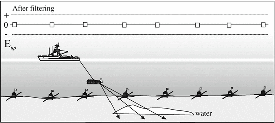
In the presence of a water reservoir, waves and energy are directly transmitted (σe ≈ σs). No wave is refracted and reflected. There is no upgoing wave; the transmission is complete
- 27.
An overview of this process is presented in the thesis of L. Loseth (2007).
- 28.
We call Green’s function, denoted G, the elementary solution of a linear differential equation or a partial derivative equation with constant coefficients. In electromagnetism, the solution is obtained using a single source (pulse or Dirac delta or δ). The general solution corresponding to the actual source is then equivalent to the superposition of impulse responses, that is to say, corresponding to the Green functions. These functions may take varied forms as, for example, analytic functions when the solution of the homogeneous differential equation is known, or an infinite series of orthogonal functions then satisfying the boundary conditions when the solution of the equation is unknown.
- 29.
Vector that indicates the direction and the sense of propagation of an electromagnetic wave. The modulus of the Poynting vector (P ≈ E∧H) corresponds to a flux, power per area unit (Skilling 1942).
- 30.
The potential vector is a mathematical tool that allows us, by introducing additional functions, to simplify the calculation procedures for the evaluation of magnetic and electric fields. For example, the fields are calculated from the potentials (specified sources), solutions of the Helmholtz equation.
- 31.
The Lorenz gauge decouples differential equations on the vector and scalar potential and then gives rise to a general solution using Green’s functions.
- 32.
Other authors have developed solutions in an infinite medium (Chave and Cox 1982).
- 33.
When the study of one of its parameters by either method produces the same result, the function is called ergodic.
- 34.
Generally these latter correspond to epiphenomena restricted in time.
- 35.
In marine exploration this could be the case above basaltic horizons or salt domes, diapirs, gas hydrates, etc. In the 1970s, very low frequency devices were proposed (Duroux 1974).
- 36.
See Chap. 4, devoted to instrumentation.
- 37.
Not to be confused with electrometer calibration, which is done on the surface ship before immersion (cf. Sect. 6.7).
- 38.
Accuracy is evaluating the absence of errors e (e = measured value – actual value). When the latter are present, the equation becomes Q e = f (P) + e, e = Q – Q e
There are two kinds of errors: time-independent (static) errors and time-dependent (dynamic) errors, which respectively are in the form e S = g(Q), e = g(Q, t)
The coherent noise is, for example, a case of dynamic error. However, there are random variations related to the environment that can only be treated by statistical methods. The arithmetic average of a finite number N of measurements is then:
$$ \overline{Q}=\frac{1}{N}{\displaystyle \sum_{i = 1}^N{Q}_i} $$The errors affecting the accuracy mainly come from the sensors, the processing and the location of the instruments (T/R). Errors can also be classified into systematic, random or accidental errors and mathematically defined. More simply, an absolute error is defined as the difference between the measurement and the true value, and a relative error as the ratio of the absolute error to the true or measured value.
- 39.
The anodes only debit when there is a loss of electrical insulation; steel is then in contact with seawater (Sainson 2007).
- 40.
Campaign led by the LETI (Commissariat for Atomic Energy) in the Mediterranean in July 1991.
- 41.
Additional measurements simultaneously realized on land.
- 42.
The means of propulsion of the ship, the shaft and propeller especially, produce (by their more or less regular rotation in sea water) alternating currents that are variable on the fundamental frequencies and their harmonics (hash of the lines of force static → modulation of the currents → BF variable fields).
- 43.
After determining the characteristic frequencies (captures and measures), electromagnetic signatures are obtained by modeling (solving Maxwell’s equations).
- 44.
Effect demonstrated for the first time in 1879 by British scientists of the Post Office Telegraph Services (Mathias et al. 1924) and seriously studied from the late 1950s (Parkinson 1959, 1962; Coquelle and Mosnier 1969; Filloux 1967; Cox and Filloux 1974; Larsen 1975; Le Mouel and Menvielle 1976; Mosnier 1977).
- 45.
EM seabed logging has not been considered practically in its principle without the help of sophisticated methods of interpretation, particularly those involving data inversion methods that have emerged in practice in the last decade. Without the latter, which require the provision of additional external information (including seismic data), the measures could not take all their senses.

References
Abrikossov I, Goutman I (1986) Géologie du pétrole. Généralités, prospection, exploitation. Ed. Mir, pp 111–114
Admundsen L et al (2006) Decomposition of electromagnetic field into up-going and down-going components. Geophysics 71(5):G211–G223
Ambronn R (1928) Elements of geophysics as applied to explorations for minerals, oil and gas. Ed. McGraw-Hill, New York, p 177
Andreis D, MacGregor L (2008) Controlled source electromagnetic sounding in shallow water. Princip Appl Geophys J 73:21–32
Archie GE (1942) The electrical resistivity log as an aid in determining some reservoir characteristics. Petrol Trans AIME 146:54–62
Bahr DE, Hutton J, Syvitski J, Pratson L (2001) Exponential approximations to compacted sediment porosity profiles. Comput Geosci 27:691–700
Bannister PR (1980) Quasi-static electromagnetic fields. Scientific and engineering studies. Ed. Naval Underwater Systems Center. Newport Laboratory
Bannister PR (1987) Simplified expressions for the electromagnetic fields of elevated, surface, or buried dipole antennas. Compiled 87, vol 1, Scientific and Engineering Studies, Naval Underwater Systems Center, New-London, Connecticut
Becker K (1985) Large scale electrical resistivity and bulck porosity of the ocean crust, deep sea drilling project hole 504B. Costa Rica rift Init Rept DSDP 83:419–427
Becquerel M (1834). Traité expérimental de l’électricité et du magnétisme et de leurs rapports avec les phénomènes naturels. Ed. Firmin Didot frères
Becquerel M, Becquerel E (1847) Elément de physique terrestre et de météorologie. Ed. Firmin Didot frères, pp 655–662
Benderitter Y, Dupis A (1969) Prospection géophysique par la méthode magnéto-tellurique, vol 4. Ed. Gauthier-Villars, Paris, pp 251–273
Bitterlich W, Wöbking H (1972) Geoelektronik. Angewandte Elektronik in der Geophysik, Geologie, Prospektion, Montanistik und Ingenieurgeologie. Ed. Springer, Berlin, pp 115–117
Born M, Wolf E (1964) Principles of optics. Electromagnetic theory of propagation, interference and diffraction of light. Ed. Pergamon Press, Oxford, 808 p
Bruck R (1841) Electricité ou magnétisme du globe terrestre. Ed Imprimerie de Delevingne and Cllewaert Tome 1:41–52
Cagniard L, Morat P (1966). Extension de la prospection magnéto-tellurique à l’exploration offshore
Chave AD (2009). On the electromagnetic field produced by marine frequency domain controlled sources. Geophys J Int:29 p
Chave AD, Cox CS (1982) Controlled electromagnetic sources for measuring electrical conductivity beneath the oceans. 1. Forward problem and model study. J Geophys Res 87(87):5327–5338
Chave AD, Luther DS (1990). Low frequency, motionally induced electromagnetic fields in the ocean. J Geophys Res 95(c5):7185–7200
Chen J, Alembaugh D (2009) Three methods for mitigating air waves in shallow water marine CSEM data. SEG Houston. International exposition and annual meeting, pp 785–789
Chouteau M, Giroux B (2006) Géophysique appliquée. Méthodes électriques. Notes de cours. Ecole Polytechnique, Montréal, p 11
Constable S (2010) Ten years of marine CSEM for hydrocarbon exploration. Geophysics 75(5):75A67–75A81
Constable S et al (2008) Mapping offshore sedimentary structure using electromagnetic methods terrain effects in marine magnetotelluric data. Geophys J Int. doi:10.1111/j.1365-246X.2008.03975.x
Coquelle J, Mosnier J (1969) Etude de l’effet « bord de mer » dans la région de Quiberon., Mémoire ENS
Cox CS, Filloux JH (1974) Two dimensional numerical models of the California electromagnetic coastal anomaly. J Geomag Geoelectr 26:257–267
Cox CS et al (1968) Electromagnetic studies of ocean currents and electrical conductivity below the ocean floor, vol 4, part I. Ed. Willey Interscience, pp 637–693
Cox CS et al (1978) Electromagnetic fluctuations induced by wind waves on the deep-seafloor. J Geophys Res 86-Cl:431–442
d’Arnaud Gerkens JC (1989) Foundation of exploration geophysics. Method in geochemistry and geophysics, vol 25. Ed. Elsevier, Amsterdam, pp 541–559
Duroux J (1974) Procédé et appareil de prospection en mer par mesure de champ électromagnétiques. Brevet français no. 74 26465
Edwards N (2005). Marine controlled source electromagnetics: principles, methodologies, future commercial applications. Survey in Geophysics, pp 675–700
Eidesmo T, Ellingrud S, MacGregor L, Constable MC, Sinha S, Johansen FN (2002) Sea bed logging (SBL), a new method for remote and direct identification of hydrocarbon filled layers in deepwater areas. First Break 20.3 March, pp 144–152
Ellingsrud S et al (2004) Electromagnetic methods and apparatus for determining the content of subterranean reservoirs. US patent no. 6696839, Feb 24
Ellis DV, Singer JM (2007) Well logging for earth scientists. Ed. Springer, p 45 et pp 222–223
England and Wales high course (2009) Decision of justice between Schlumberger Holding Ltd and Electromagnetic Geoservices As (EMGS), p 5
Evjen HM (1938) Depth factors and resolving power of electrical measurements. Geophysics 3(1–4):78–95
Fielding BJ, Lu X (2009) System and method for towing sub-sea vertical antenna. US patent no. 7541996, June 2
Filloux JH (1967) Oceanic electric currents, geomagnetic variations and the deep electrical conductivity structure of the ocean-continent transition of central California. PhD thesis, University of California, San Diego
Filloux JH (1987) Instrumentation and experimental methods for oceanic studies. Geomagnetism, vol 1. Ed. Jacob, pp 143–248
Fofonoff N, Millard RC (1983) Algorithms for computation of fundamental properties of seawater. UNESCO Tech Pap Mat Sci 44, 53 pp
Grand FS, West GF (1965) Interpretation theory in applied geophysics. McGraw-Hill, New York
Guegen Y (1997) Introduction à la physique des roches. Ed. Hermann, Paris
Guérin R (2007) Profondeur d’investigation en imagerie de résistivité électrique. 8ème colloque GEOFCAN, Bondy, France, 25–26 September, pp 27–30
Guibert A (2009) Diagnostic de corrosion et prédiction de signature électromagnétique de structures sous-marines sous protection cathodique. Doctoral thesis, Université de Grenoble, 218 p
Hamon BV (1958) The effect of pressure on the electrical conductivity of the seawater. J Mar Res 16:83–86
Harrington RF (1961) Time harmonic electromagnetic field. McGraw-Hill, New York, 480 p
Heaviside O (1899). Note on the electrical waves in seawater. Electromagnetic theory, pp 536–537. Ed. E. Benn
Heshammer J, Fanavoll S, Stefatos A, Danielsen J E and Boulaenko M (2010) CSEM performance in light of well results. The Leading Edge, January, pp 258–264
Horne RA, Frystinger CR (1963) The effect of pressure on the electric conductivity of the seawater. J Geophys Res 68:1967–1973
Ingmanson DE, Wallace WJ (1989) Oceanography: an introduction, 4th edn. Ed. Wadsworth Publishing, Belmont
Jackson JD (1998) Classical electrodynamics. Ed. Wiley, New York
Jiracek GR (1990) Near surface and topographic distortions in electromagnetic induction. Survey Geophys 11:162–203
Johansen et al (2008) How EM survey analysis validates current technology, processing and interpretation methodology. First Break 26, June, pp 83–88
Kaushalendra Mangal Bhatt (2011) Motion induced noise in marine electromagnetic data. Thèse
Key K (2009) 1D inversion of multicomponent, multifrequency marine CSEM data: methodology and synthetic studies for resolving thin resistive layers. Geophysics 74(2):F9–F20
Key K, Lockwood A (2010) Determining the orientation of marine CSEM receivers using orthogonal procrustes rotation analysis. Geophysics 75(3)
Kiyoshi B, Nobukazu S (2002) A new technique for incorporation of seafloor topography in electromagnetic modelling. Geophys J Int 150:392–402
Knudsen M (1901) Hydrografische, Tabellenth edn. Friedrichsen, Hamburg, 63 p
Kong JA (1986) Electromagnetic wave theory. Wiley, New York
Kong FN et al (2009) Casing effects in the sea-to-borehole electromagnetic method. Geophysics 14(5):F77–F87
Kraichman MB (1976) Handbook of electromagnetic propagation in conducting media. Ed. Navy Department Bureau of Ships, Appendix A.4
Kunetz G (1966) Principles of direct current resistivity prospecting. Ed. Bebruder Borntraeger, Berlin, p 9
Landau L, Lifchitz E (1969) Electrodynamique des milieux continus. Ed. Mir, Moscou, pp 150 and 352
Larsen JC (1975) Low frequency (0.1–6.0 cpd) electromagnetic study of deep mantle electrical conductivity beneath the Hawaiian Islands. Geophys J R Astr Soc 43:17–46
Le Mouel JL, Menvielle M (1976) Geomagnetic variation anomalies and deflection of telluric currents. Geophys J R Astron Soc 68:575–587
Li Y, Constable S (2007) Marine control source: 2D marine controlled source electromagnetic modelling. Part 2: effect of bathymetry. Geophysics 72(2):63–71
Li YG, Constable S (2010) Transient electromagnetic in shallow water: insights from 1D modelling. Chin J Geophys 53:737–742
Lodge OJ (1892) Modern views of electricity. Nature series. Ed. Macmillan, London, p 94
Loseth LO (2007) Modeling of controlled source electromagnetic data. PhD thesis, Université norvégienne, pp 167–168
Loseth LO et al (2006) Low frequency electromagnetic fields in applied geophysics: waves or diffusion? Geophysics 71(4):W29–W40
MacGillivray PR, Oldenburg DW (1990) Methods for calculating Fréchet derivatives and sensitivities for non-linear inverse problem: a comparative study. Geophys Prospect 38(5):403–416
MacGregor L, Andreis D, Tompkins M (2007) Electromagnetic surveying for resistive or conductive bodies. US patent no. 2007/0288211, December 13
MacGregor L et al (2008) Electromagnetic surveying for hydrocarbon reservoirs. US patent no. 7,337,064, Feb 26
Meyer JJ et al (1969) Handbook of ocean and underwater engineering. Ed. McGraw-Hill, New York, p 3.38
Mittet R (2008) Normalized amplitude ratios for frequency domain CSEM in very shallow water. First Break 26:47–54
Mosnier J (1977) Le sondage magnétique différentiel. Courrier du CNRS, no. 26, October, pp 6–14
Nover G (2005) Electrical properties of crustal and mantle Rocks : a review of laboratory measurements and their explanation. Survey in geophysics, vol 26. Ed. Springer, pp 593–651
Ohm GS (1827) Die galvanische Kette, mathematisch bearbeitet. Ed. TH Riemann, Berlin, 246 p
Parkhomenko EI (1967) Electrical properties of rocks. Ed. Plenum Press, New York, 314 p
Parkinson WD (1959) Direction of rapid geomagnetic fluctuations. Geophys J R Astron Soc 2:1–14
Parkinson WD (1962) The influence of continents and oceans on geomagetic variations. Geophys J R Astron Soc 4:441–449
Pavlov D et al (2009). Method for phase and amplitude correction in controlled source electromagnetic survey data. US patent no. 2009/0133870. May 28
Pirson JP (1950) Element of oil reservoir engineering. Ed. McGraw-Hill, New York, p 58
Price A, Mikkelsen G, Halmilton M (2010) 3D CSEM over Frigg: dealing with cultural noise. SEG Denver, annual meeting, pp 670–674
Razafindratsima S et al (2006) Influence de la teneur en eau sur les propriétés électriques complexes des matériaux argileux. Laboratoire IRD/UMPC
Robert M (1959) Géologie des pétroles. Principes et applications. Ed. Gauthier-Villars, pp 87–90
Rosten T, Admundsen L (2008) Electromagnetic wave field analysis. UK patent no. 2412739
Rosten T et al (2005) Electromagnetic seabed logging: a proven tool for direct hydrocarbon identification. OTC paper 17483, Houston, 5 p
Rubin Y, Hubbard S (2006) Hydrogeophysics. Water science and technology library. Ed. Springer, Dordrecht, p 196
Sainson S (2007). Inspection en ligne des pipelines. Principes et méthodes. Ed. Tec et Doc, Lavoisier, pp 231–242 and pp 73–74
Sainson S (2008) EM response to conductive structures immerged in conductive media. Confidential report
Sainson S (2009) EM subsea pipelines effect on mCSEM survey. Confidential report
Sainson S (2010) Les diagraphies de corrosion. Acquisition et interprétation des données. Ed. Tec et Doc, Lavoisier, pp 77–81
Schermber JL (2006) Identification et caractérisation de sources électromagnétiques. Application à la discrétion des moteurs de propulsion navale. Doctoral thesis, Université de Grenoble, 229 p
Seguin MK (1971) La géophysique et les propriétés physiques des roches. Ed. Les presses de l’université de Laval, Québec, p 130
Serra O (2004) Well logging, vol 1 Data acquisitions and applications. Ed. Technip, 688 p
Skilling HH (1942) Fundamentals of electric waves. Ed. Wiley, pp 118–122
Stefatos et al (2009) Marine CSEM technology performances in hydrocarbon exploration: limitations or opportunities. First Break 27, May, pp 65–71
Stratton JA (1961) Electromagnetic theory. Ed McGraw-Hill, p 314 et p 374
Sunde ED (1948) Earth conduction effects in transmission systems. Ed. D Van Nostrand, New York, p 20
Theys P (2006) Utilisations des données pétrophysiques en temps réel et pendant toute la vie d’un champ: critères de qualité et d’éthique. Communication SAID (SPWLA), Schlumberger, Clamart, 5 April
Thomsen, Menache (1954) Instructions pratiques sur la détermination de a salinité de l’eau de mer par la méthode de Mohr-Knudsen. Bulletin de l’institut océanographique, no. 1047, 30 July
Tompkins MJ, Weaver R, MacGregor LM (2004) Sensitivity to hydrocarbon targets using marine active source EM sounding: diffusive EM imaging methods. EAGE. Ed. OHM
Von Aulock W (1953) The electromagnetic field of an infinite cable in seawater. Bureau of Ships Minesweeping Branch technical report, no. 106
Walker PW, West GF (1992) Parametric estimators for current excitation on a thin plate. Geophysics 57:766–773
Warburton F, Caminiti R (1964) Champ magnétique induit par les vagues de la mer. Bull Am Phys Soc 2(3):347
Webster AG (1897) The theory of electricity and magnetism being lectures on mathematical physics. Ed Macmillan, London, pp 534–540
Weiss CJ (2007) The fallacy of the shallow water problem in marine CSEM exploration. Geophysics 72(6):A93–A97
Whitchead CS (1897) The effect of seawater on induction telegraphy. Physical Society
Author information
Authors and Affiliations
Rights and permissions
Copyright information
© 2017 Springer International Publishing Switzerland
About this chapter
Cite this chapter
Sainson, S. (2017). Metrology and Environment. In: Electromagnetic Seabed Logging. Springer, Cham. https://doi.org/10.1007/978-3-319-45355-2_3
Download citation
DOI: https://doi.org/10.1007/978-3-319-45355-2_3
Published:
Publisher Name: Springer, Cham
Print ISBN: 978-3-319-45353-8
Online ISBN: 978-3-319-45355-2
eBook Packages: Earth and Environmental ScienceEarth and Environmental Science (R0)