Introductory Theory of Interferometry and Synthesis Imaging

Abstract

In this chapter, we provide a simplified analysis of interferometry and introduce several important concepts. We first consider an interferometer in one dimension and discuss the effect of finite bandwidth and show how the interferometer response can be interpreted as a convolution. We extend the analysis to two dimensions and discuss circumstances in which three-dimensional imaging can be undertaken. This chapter is intended to provide a broad introduction to the principles of synthesis imaging to facilitate the understanding of more detailed development in later chapters. A brief introduction to the theory of Fourier transforms is given in Appendix 2.1.

In this chapter, we provide a simplified analysis of interferometry and introduce several important concepts. We first consider an interferometer in one dimension and discuss the effect of finite bandwidth and show how the interferometer response can be interpreted as a convolution. We extend the analysis to two dimensions and discuss circumstances in which three-dimensional imaging can be undertaken. This chapter is intended to provide a broad introduction to the principles of synthesis imaging to facilitate the understanding of more detailed development in later chapters. A brief introduction to the theory of Fourier transforms is given in Appendix 2.1.

2.1 Planar Analysis

The instantaneous response of a radio interferometer to a point source can most simply be analyzed by considering the signal paths in the plane containing the electrical centers of the two interferometer antennas and the source under observation. For an extended observation, it is necessary to take account of the rotation of the Earth and consider the geometric situation in three dimensions, as can be seen from Fig. 1.15 However, the two-dimensional geometry is a good approximation for short-duration observations, and the simplified approach facilitates visualization of the response pattern.

Consider the geometric situation shown in Fig. 2.1, where the antenna spacing is east–west. The two antennas are separated by a distance D, the baseline, and observe the same cosmic source, which is in the far field of the interferometer; that is, it is sufficiently distant that the incident wavefront can be considered to be a plane over the distance D. The source will be assumed for the moment to have infinitesimal angular dimensions. For this discussion, the receivers will be assumed to have narrow bandpass filters that pass only signal components very close to ν.

Fig. 2.1

Geometry of an elementary interferometer. D is the interferometer baseline.

As explained for the phase-switching interferometer in Chap. 1, the signal voltages are multiplied and then time-averaged, which has the effect of filtering out high frequencies. The wavefront from the source in direction θ reaches the right antenna at a time

$$\displaystyle{ \tau _{g} = \frac{D} {c} \sin \theta }$$

(2.1)

before it reaches the left one. τ _g is called the geometric delay, and c is the velocity of light. Thus, in terms of the frequency ν, the output of the multiplier is proportional to

$$\displaystyle\begin{array}{rcl} F& =& 2\sin (2\pi \nu t)\sin 2\pi \nu (t -\tau _{g}) \\ & =& 2\sin ^{2}(2\pi \nu t)\cos (2\pi \nu \tau _{ g}) - 2\sin (2\pi \nu t)\cos (2\pi \nu t)\sin (2\pi \nu \tau _{g})\;.{}\end{array}$$

(2.2)

The center frequency of the receivers is generally in the range of tens of megahertz to hundreds of gigahertz. As the Earth rotates, the most rapid rate of variation of θ is equal to the Earth’s rotational velocity, which is of the order of 10⁻⁴ rad s⁻¹. Also, because D cannot be more than, say, 10⁷ m for terrestrial baselines, the rate of variation of ν τ _g is smaller than that of ν t by at least six orders of magnitude. For an averaging period T ≫ 1∕ν, the average value of $\sin ^{2}(2\pi \nu t) = \frac{1} {2}$ and the average value of sin(2π ν t)cos(2π ν t) = 0, leaving the fringe function

$$\displaystyle{ F =\cos 2\pi \nu \tau _{g} =\cos \left (\frac{2\pi Dl} {\lambda } \right )\;, }$$

(2.3)

where l = sinθ; the definition of the variable l is discussed further in Sect. 2.4. For sidereal sources, the variation of θ with time as the Earth rotates generates quasisinusoidal fringes at the correlator, which are the output of the interferometer. Figure 2.2 shows an example of this function, which can be envisaged as the directional power reception pattern of the interferometer for the case in which the antennas either track the source or have isotropic responses and thus do not affect the shape of the pattern.

Fig. 2.2

Polar plot to illustrate the fringe function F = cos(2π D l∕λ). The radial component is equal to | F | , and θ is measured with respect to the vertical axis. Alternate lobes correspond to positive and negative half-cycles of the quasi-sinusoidal fringe pattern, as indicated by the plus and minus signs. To simplify the diagram, a very low value of 3 is used for D∕λ. The increase in fringe width due to foreshortening of the baseline as | θ | increases is clearly shown. The maxima in the horizontal direction (θ = ±90^∘) are a result of the arbitrary choice of an integer value for D∕λ.

An alternate and equivalent way of envisaging the formation of the sinusoidal fringes is to note that because of the rotation of the Earth, the two antennas have different components of velocity in the direction of the source. The signals reaching the antennas thus suffer different Doppler shifts. When the signals are combined in the multiplying action of the receiving system, the sinusoidal output arises from the beats between the Doppler-shifted signals.

A development of the simple analysis can be made if we consider two Fourier components of the received signal at frequencies ν ₁ and ν ₂. These frequency components are statistically independent so that the interferometer output is the linear sum of the responses to each component. Hence, the output has components F ₁ and F ₂, as in Eq. (2.3). For frequency ν ₂, the coefficient 2π D∕λ = 2π D ν ₂∕c will be different from that for ν ₁, so F ₂ will have a different period from F ₁ at any given angle θ. This difference in period gives rise to interference between F ₁ and F ₂, so that the fringe maxima have superimposed on them a modulation function that also depends on θ. Similar effects occur in the case of a continuous band of frequencies. For example, if the signals at the correlator are of uniform power spectral density over a band of width Δ ν and center frequency ν ₀, the output becomes

$$\displaystyle\begin{array}{rcl} F(l)& =& \frac{1} {\varDelta \nu } \int _{\nu _{0}-\varDelta \nu /2}^{\nu _{0}+\varDelta \nu /2}\cos \left (\frac{2\pi Dl\nu } {c} \right )d\nu \\ & =& \cos \left (\frac{2\pi Dl\nu _{0}} {c} \right )\ \frac{\sin (\pi Dl\varDelta \nu /c)} {\pi Dl\varDelta \nu /c} \;.{}\end{array}$$

(2.4)

Thus, the fringe pattern has an envelope in the form of a sinc function [sinc(x) = (sinπ x)∕π x]. This is an example of the general result, to be discussed in the following section, that in the case of uniform power spectral density at the antennas, the envelope of the fringe pattern is the Fourier transform of the instrumental frequency response.

2.2 Effect of Bandwidth

Figure 2.3 shows an interferometer of the same general type as in Fig. 2.1 but with the amplifiers H₁ and H₂, the multiplier, and an integrator (with respect to time) shown explicitly. An instrumental time delay τ _i is inserted into one arm. Assume that for a point source, each antenna delivers the same signal voltage V (t) to the correlator, and that one voltage lags the other by a time delay τ = τ _g −τ _i , as determined by the baseline D and the source direction θ. The integrator within the correlator has a time constant 2T; that is, it sums the output from the multiplier for 2T seconds and then resets to zero after the sum is recorded. The output of the correlator may be a voltage, a current, or a coded set of logic levels, but in any case, it represents a physical quantity with the dimensions of voltage squared.

Fig. 2.3

Elementary interferometer showing bandpass amplifiers H₁ and H₂, the geometric time delay τ _g , the instrumental time delay τ _i , and the correlator consisting of a multiplier and an integrator.

The output from the correlator resulting from a point source¹ is

$$\displaystyle{ r = \frac{1} {2T}\int _{-T}^{T}V (t)V (t-\tau )\;dt\;. }$$

(2.5)

We have ignored system noise and assumed that the two amplifiers have identical bandpass characteristics, including finite bandwidths Δ ν outside which no frequencies are admitted. The integration time 2T is typically milliseconds to seconds, that is, very much larger than Δ ν ⁻¹. Thus, Eq. (2.5) can be written as

$$\displaystyle{ r(\tau ) =\lim _{T\rightarrow \infty } \frac{1} {2T}\int _{-T}^{T}V (t)V (t-\tau )\;dt\;, }$$

(2.6)

which is an (unnormalized) autocorrelation function. The condition T → ∞ is satisfied if a large number of variations of the signal amplitude, which have a duration ∼ Δ ν ⁻¹, occur in time 2T. The integration time used in practice must clearly be finite and much less than the fringe period.

As described in Chap. 1, the signal from a natural cosmic source can be considered as a continuous random process that results in a broad spectrum, of which the phases are a random function of frequency. It will be assumed for our immediate purpose that the time-averaged amplitude of the cosmic signal in any finite band is constant with frequency over the passband of the receiver.

The squared amplitude of a frequency spectrum is known as the power density spectrum, or power spectrum. The power spectrum of a signal is the Fourier transform of the autocorrelation function of that signal. This statement is known as the Wiener–Khinchin relation (see Appendix A2.1.5) and is discussed further in Sect. 3.2 It applies to signals that are either deterministic or statistical in nature and can be written

$$\displaystyle{ \big\vert H(\nu )\big\vert ^{2} =\int _{ -\infty }^{\infty }r(\tau )e^{-j2\pi \nu \tau }d\tau \;, }$$

(2.7)

and

$$\displaystyle{ r(\tau ) =\int _{ -\infty }^{\infty }\big\vert H(\nu )\big\vert ^{2}e^{j2\pi \nu \tau }d\nu \;, }$$

(2.8)

where H(ν) is the amplitude (voltage) response, and hence | H(ν) | ² is the power spectrum of the signal input to the correlator. In this case, because the cosmic signal is assumed to have a spectrum of constant amplitude, the spectrum H(ν) is determined solely by the passband characteristics (frequency response) of the receiving system from the outputs of the antennas to the output of the integrator. Thus, the output of the interferometer as a function of the time delay τ is the Fourier transform of the power spectrum of the cosmic signal as bandlimited by the receiving system. Assume, as a simple example, a Gaussian passband centered at ν ₀:

$$\displaystyle{ \big\vert H(\nu )\big\vert ^{2} = \frac{1} {2\sigma \sqrt{2\pi }}\left \{\exp \left [-\frac{(\nu -\nu _{0})^{2}} {2\sigma ^{2}} \right ] +\exp \left [-\frac{(\nu +\nu _{0})^{2}} {2\sigma ^{2}} \right ]\right \}\;, }$$

(2.9)

where σ is the bandwidth factor (the full bandwidth at half-maximum level is $\sqrt{ 8\ln 2}\,\sigma$). Note that to perform the Fourier transforms in Eqs. (2.7) and (2.8), we include a negative frequency response centered on −ν ₀. The spectrum is then symmetrical with respect to zero frequency, which is consistent with the fact that the autocorrelation function (which is the Fourier transform of the power spectrum) is real. The negative frequencies have no physical meaning but arise mathematically from the use of the exponential function. The interferometer response is

$$\displaystyle{ r(\tau ) = e^{-2\pi ^{2}\tau ^{2}\sigma ^{2} }\cos (2\pi \nu _{0}\tau )\;, }$$

(2.10)

which is illustrated in Fig. 2.4a. Note that r(τ) is a cosinusoidal function multiplied by an envelope function, in this case a Gaussian, whose shape and width depend on the amplifier passband. This envelope function is referred to as the delay pattern or bandwidth pattern.

Fig. 2.4

Point-source response of an interferometer with (a ) Gaussian and (b ) rectangular passbands. The abscissa is the geometric delay τ _g . The bandwidth pattern determines the envelope of the fringe term.

By setting the instrumental delay τ _i to zero and substituting for the geometric delay τ _g  = (D∕c)sinθ in Eq. (2.10), we obtain the response

$$\displaystyle{ r(\tau _{g}) = \text{exp}\left [-2\left (\frac{\pi D\sigma } {c} \,\sin \theta \right )^{2}\right ]\cos \left (\frac{2\pi \nu _{0}D} {c} \sin \theta \right )\;. }$$

(2.11)

The period of the fringes (the cosine term) varies inversely as the quantity ν ₀ D∕c = D∕λ and does not depend on the bandwidth parameter σ. The width of the bandwidth pattern (the exponential term), however, is a function of both σ and D ; wide bandwidths and long baselines result in narrow fringe envelopes. This result is quite general. For example, a rectangular amplifier passband of width Δ ν, as considered in Eq. (2.4), results in an envelope pattern of the form [sin(π Δ ν τ)]∕(π Δ ν τ), as shown in Fig. 2.4b.

In imaging applications, it is usually desirable to observe the fringes in the vicinity of the maximum of the pattern, where the fringe amplitude is greatest. This condition can be achieved by changing the instrumental delay τ _i continuously or periodically so as to keep τ = τ _g −τ _i suitably small. If τ _i is adjusted in steps of the reciprocal of the center frequency² ν ₀, the response remains cosinusoidal with τ _g . Note that for wide bandwidths, as Δ ν approaches ν, the width of the envelope function becomes so narrow that only the central fringe remains. This occurs mainly in optics, where a central fringe of this type is often called the “white light” fringe.

2.3 One-Dimensional Source Synthesis

In the analysis of an interferometer in which the antennas and the instrumental delay track the position of the source, as is the norm for frequencies above ∼ 1 GHz, it is convenient to specify angles of the antenna beam and other variables with respect to a reference position on the sky, usually the center or nominal position of the source under observation. This is commonly referred to as the phase reference position. Since the range of angles required to specify the source intensity distribution relative to this point is generally no more than a few degrees, small-angle approximations can be used to advantage. The instrumental delay is constantly adjusted to equal the geometric delay for radiation from the phase reference position. If we designate this reference position as the direction θ ₀, then τ _i  = (D∕c)sinθ ₀. For radiation from a direction (θ ₀ −Δ θ), where Δ θ is a small angle, the fringe response term is

$$\displaystyle\begin{array}{rcl} \cos (2\pi \nu _{0}\tau )& =& \cos \left \{2\pi \nu _{0}\left [\frac{D} {c} \sin (\theta _{0}-\varDelta \theta ) -\tau _{i}\right ]\right \} \\ & \simeq & \cos [2\pi \nu _{0}(D/c)\sin \varDelta \theta \cos \theta _{0}]{}\end{array}$$

(2.12)

for cosΔ θ ≃ 1. When observing a source at any position in the sky, the angular resolution of the fringes is determined by the length of the baseline projected onto a plane normal to the direction of the source. In Fig. 2.1, for example, this is the distance designated Dcosθ. We therefore introduce a quantity u that is equal to the component of the antenna spacing normal to the direction of the reference position θ ₀. u is measured in wavelengths, λ, at the center frequency ν ₀, that is,

$$\displaystyle{ u = \frac{D\cos \theta _{0}} {\lambda } = \frac{\nu _{0}D\cos \theta _{0}} {c} \;. }$$

(2.13)

Since Δ θ in Eq. (2.12) is small, we can assume that the bandwidth pattern is near maximum (unity) in the direction θ ₀ −Δ θ. Then, from Eqs. (2.12) and (2.13), the response to radiation from that direction is proportional to

$$\displaystyle{ F(l) =\cos (2\pi \nu _{0}\tau ) =\cos (2\pi ul)\;, }$$

(2.14)

where l = sinΔ θ. This is the response to a point source at θ = θ ₀ −Δ θ of an interferometer whose net delay τ _g −τ _i is zero at θ = θ ₀. As we shall show, the quantity u is interpreted as spatial frequency. It can be measured in cycles per radian, since the spatial variable l, being small, can be expressed in radians.

2.3.1 Interferometer Response as a Convolution

The response of a single antenna or an interferometer to a source can be expressed in terms of a convolution. Consider first the response of a single antenna and a receiver that measures the power received. Figure 2.5 shows the power reception pattern of the antenna A(θ), which is a polar plot of the effective area of the antenna as a function of angle from the center of the antenna beam. Also shown is the one-dimensional intensity profile of a source I ₁(θ′), as defined in Eq. (1.9), in which θ′ is measured with respect to the center, or nominal position, of the source. The component of the output power in bandwidth Δ ν contributed by each element d θ′ of the source is $\frac{1} {2}\varDelta \nu A(\theta '-\theta )I_{1}(\theta ')d\theta '$, where the factor $\frac{1} {2}$ takes account of the ability of the antenna to respond to only one component of randomly polarized radiation. The total output power from the antenna, omitting the constant factor $\frac{1} {2}\varDelta \nu$, is proportional to

$$\displaystyle{ \int _{\text{source}}A(\theta '-\theta )I_{1}(\theta ')d\theta '\;. }$$

(2.15)

This integral is equal to the cross-correlation of the antenna reception pattern and the intensity distribution of the source. It is convenient to define $\mathcal{A}(\theta ) = A(-\theta )$, where $\mathcal{A}$ is the mirror image of A with respect to θ. Then expression (2.14) becomes

$$\displaystyle{ \int _{\text{source}}\mathcal{A}(\theta -\theta ')I_{1}(\theta ')d\theta '\;. }$$

(2.16)

The integral in expression (2.15) is an example of the convolution integral; see Appendix 2.1, Eq. (A2.33). We can say that the output power of the antenna is given by the convolution of the source with the mirror image of the power reception pattern of the antenna. The mirror-image³ reception pattern can be described as the response of the antenna to a point source.

Fig. 2.5

The power pattern A(θ) of an antenna pointed in the direction OC, and the intensity profile of a source I ₁(θ′), used to illustrate the convolution relationship. The angle θ is measured with respect to the beam center OC. The profile of the source is a function of θ′, measured with respect to the direction of the nominal position of the source OB.

In the case of an interferometer, we can express the response as a convolution by replacing the antenna power pattern in Eq. (2.16) by the overall power pattern of the interferometer. From the results presented earlier, we find that the response of an interferometer is determined by three functions:

• The reception pattern of the antennas, which we represent as A(l),

• The fringe pattern, F(l), as in the example of Fig. 2.2 and given by Eq. (2.14). Note that the fringe term in the interferometer output, being the product of two voltages, is proportional to power.

• The bandwidth pattern, for example, as given by the sinc-function factor in Eq. (2.4). In the general case, we can represent this by F _B (l).

Note that the antenna beam is often symmetrical, in which case, if the interferometer fringes are aligned with the beam center, we can disregard the distinction between the interferometer power pattern and its mirror image in using the convolution relationship.

Next, consider an interferometer with tracking antennas and an instrumental delay that is adjusted so the bandwidth pattern also tracks the source across the sky. In effect, the intensity distribution is modified by the antenna and bandwidth patterns. We can therefore envisage the output of the interferometer as the convolution of (the mirror image of) the fringe pattern with the modified intensity. In terms of the convolution integral, the response can be written as

$$\displaystyle{ R(l) =\int _{\text{source}}\cos \left [2\pi u(l - l')\right ]A(l')F_{B}(l')I_{1}(l')dl'\;. }$$

(2.17)

or, more concisely,

$$\displaystyle{ R(l) =\cos (2\pi ul) {\ast} [A(l)F_{B}(l)I_{1}(l)]\;, }$$

(2.18)

where the in-line asterisk symbol (∗) denotes convolution. The intensity distribution measured with the interferometer is modified by A(l) and F _B (l), but since these are measurable instrumental characteristics, I ₁(l) can generally be recovered from the product A(l)F _B (l)I ₁(l). In many cases, the angular size of the source is small compared with the antenna beams and the bandwidth pattern, so these two functions introduce only a constant in the expression for the response. To simplify the discussion, we shall consider this case, and omitting constant factors, we can write the essential response of the interferometer as

$$\displaystyle{ R(l) =\cos (2\pi ul) {\ast} I_{1}(l)\;. }$$

(2.19)

In the case of the early interferometer shown in Fig. 1.6, in which the antennas are fixed in the meridian and do not track the source, the delays in the signal paths between the antennas and the point at which the signals are multiplied are equal, and there is no variable instrumental delay. Thus, the three functions that determine the interferometer power pattern are all fixed with respect to the interferometer baseline. The interferometer power pattern is of the form A(l)cos(2π u l)F _B (l), and the response of the interferometer to the source is [A(l)cos(2π u l)F _B (l)] ∗ I ₁(l).

Most interferometers for operation at meter wavelengths, that is, at frequencies below about 300 MHz, use antennas that are arrays of fixed dipoles. At such long wavelengths, it is possible to obtain large collecting areas and still have wide enough beams that some minutes of observing time are obtained as a source passes through in sidereal motion. Often the bandwidth of such low-frequency instruments is small, so that the bandwidth pattern, F _B (l), is wide and this factor can be omitted. Also, the antenna beams are usually wider than the source and sufficiently wide that several cycles of the fringe pattern can be measured as the source transits the beam. So in the nontracking case, the essential form of the response is also represented by Eq. (2.19). However, fixed antennas with nontracking beams are mainly a feature of the early years of radio astronomy, and in more recent meter-wavelength arrays, the phases of individual dipoles, or small clusters of dipoles, can be adjusted to provide steerable beams.

2.3.2 Convolution Theorem and Spatial Frequency

We now examine the interferometer response, as given in Eq. (2.19), using the convolution theorem of Fourier transforms (see the derivation in Appendix A2.1.2), which can be expressed as:

$$\displaystyle{ f {\ast} g\longleftrightarrow FG\;, }$$

(2.20)

where f ↔ F, g ↔ G, and ↔ indicates Fourier transformation. Consider the Fourier transforms with respect to l and u of the three functions in Eq. (2.19). For the interferometer response, we have r(u) ↔ R(l). For a particular value u = u ₀, the Fourier transform of the fringe term is given by [see Fourier transform example in Eq. (A2.15)]

$$\displaystyle{ \cos (2\pi u_{0}l)\longleftrightarrow \frac{1} {2}\left [\delta (u + u_{0}) +\delta (u - u_{0})\right ]\;, }$$

(2.21)

where δ is the delta function defined in Appendix 2.1. The Fourier transform of I ₁(l) is the visibility function $\mathcal{V}(u)$. Thus, from Eqs. (2.19), (2.20), and (2.21), we obtain

$$\displaystyle\begin{array}{rcl} r(u)& = \frac{1} {2}\left [\delta (u + u_{0}) +\delta (u - u_{0})\right ]\mathcal{V}(u)& \\ & = & \frac{1} {2}\left [\mathcal{V}(-u_{0})\delta (u + u_{0}) + \mathcal{V}(u_{0})\delta (u - u_{0})\right ]\;.{}\end{array}$$

(2.22)

This result shows that the instantaneous output of the interferometer as a function of spatial frequency consists of two delta functions situated at plus and minus u ₀ on the u axis. Now, $\mathcal{V}(u)$, the Fourier transform of I ₁(l), represents the amplitude and phase of the sinusoidal component of the intensity profile with spatial frequency u cycles per radian. The interferometer acts as a filter that responds only to spatial frequencies ± u ₀. The negative spatial frequency − u ₀ has no physical meaning. It arises from the use, for mathematical convenience, of the exponential Fourier transform rather than the sine and cosine transforms, which correspond more directly to the physical situation. As a result, the spatial frequency spectra are symmetrical about the origin in the Hermitian sense, that is, with even real parts and odd imaginary parts, which is appropriate since the intensity is a real, not complex, quantity.

Fringe visibility, as originally defined by Michelson [$\mathcal{V}_{M}$, see Eq. (1.9)], is a real quantity and is normalized to unity for an unresolved source. Complex visibility (Bracewell 1958) was defined to take account of the phase of the visibility, measured as the fringe phase, to allow imaging of asymmetric and complicated sources. The normalization is convenient when comparing measurements with simple models, as shown in Fig. 1.5 However, in images, it is desirable to display the magnitude of the intensity or brightness temperature, so the general practice is to retain the measured value of visibility, without normalization, since this incorporates the required information. Thus, visibility $\mathcal{V}$ as used here is an unnormalized complex quantity with units of flux density (W m⁻² Hz⁻¹). The quantity u, which was introduced as the projected baseline in wavelengths, is seen also to represent the spatial frequency of the Fourier components of the intensity. The concepts of spatial frequency and spatial frequency spectra are fundamental to the Fourier synthesis of astronomical images, and this general subject is discussed in a seminal paper by Bracewell and Roberts (1954).

2.3.3 Example of One-Dimensional Synthesis

To illustrate the observing process outlined in this chapter, we present a rudimentary simulation of measurements of the complex visibility of a source using arbitrary parameters. The source consists of two components separated by 0. 34^∘ of angle, the flux densities of which are in the ratio 2: 1. The measurements are made with pairs of antennas placed along a line parallel to the direction of separation of the two components. Measurements are made for antenna spacings that are integral multiples of a unit spacing of 30 wavelengths. All spacings from 1 to 23 times the unit spacing are measured. These results could be obtained using two antennas and a single correlator, observing the source as it transits the meridian on 23 different days and moving the antennas to provide a new spacing each day. Alternately, the 23 measurements could be made simultaneously using 23 correlators and a number of antennas that could be as small as 8 (if they were set out with minimum redundancy in the spacings, as discussed in Sect. 5.5). The angular sizes of the two components of the source are too small to be resolved by the interferometer, so they can be regarded as point radiators. The two components radiate noise, and their two outputs are uncorrelated. The source is at a sufficient distance that incoming wavefronts can be considered to be plane over the measurement baselines.

Figure 2.6a and b show, respectively, the amplitude⁴ and phase of the visibility function as it would be measured. Since the data are derived from a model, there are no measurement errors, so the points indicate samples of the Fourier transform of the source intensity distribution, which can be represented by two delta functions with strengths in the ratio 1: 2. Taking the inverse transform of the visibility yields the synthesized image of the source in Fig. 2.6c. The two components of the source are clearly represented. The extraneous oscillations arise from the finite extent of the visibility measurements, which are uniformly weighted out to a cutoff at 23 times the unit spacing. This effect is further illustrated in Fig. 2.6d, which shows the response of the measurement procedure to a single point source; equivalently, it is the synthesized beam. The profile of this response is the sinc function that is the Fourier transform of the rectangular window function, which represents the cutoff of the measurements at the longest spacing. In the image domain, the double-source profile can be viewed as the convolution of the source with the point-source response. The point-source nature of the model components maximizes the sidelobe oscillations, which would be partially smoothed out if the width of the components were comparable to that of the sidelobes.

Fig. 2.6

Simulated measurements of visibility of a double source: (a ) visibility amplitude and (b ) visibility phase, each plotted as a function of antenna spacing as a multiple of the unit spacing; (c ) the profile derived from the measurements and (d ) the response to a point source.

As is clear from the convolution relationship, information on the structure of the source is contained in the whole response pattern in Fig. 2.6c, that is, in the sidelobe oscillations as well as the main-beam peaks. A way to extract the maximum information on the source structure would be to fit scaled versions of the response in Fig. 2.6d to the two peaks in Fig. 2.6c and then subtract them from the profile. In an actual observation, this would leave the noise and any structure that might be present in addition to the point sources but would remove all or most of the sidelobes. The fitting of the point-source responses could be adjusted to minimize some measure of the residual fluctuations, and further components could be fitted to any remaining peaks and subtracted. This technique would clearly be a good way to estimate the strengths and positions of the two components and to look for evidence of any low-level structure that could be hidden by the sidelobes in Fig. 2.6c. The CLEAN algorithm, which is discussed in Chap. 11, uses this principle but also replaces the components that are removed by model beam responses that are free of sidelobes. Removal of the sidelobes allows any lower-level structure to be investigated, down to the level of the noise. Most synthesis images are processed by nonlinear algorithms of this type, and the range of intensity levels achieved in some two-dimensional images exceeds 10⁵ to 1.

2.4 Two-Dimensional Synthesis

Synthesis of an image of a source in two dimensions on the sky requires measurement of the two-dimensional spatial frequency spectrum in the (u, v) plane, where v is the north–south component as shown in Fig. 2.7a. Similarly, it is necessary to define a two-dimensional coordinate system (l, m) on the sky. The (l, m) origin is the reference position, or phase reference position, introduced in the last section. In considering functions in one dimension in the earlier part of this chapter, it was possible to define l in Eq. (2.3) as the sine of an angle. In two-dimensional analysis, l and m are defined as the cosines of the angles between the direction (l, m) and the u and v axes, respectively, as shown in Fig. 2.7c. If the angle between the direction (l, m) and the w axis is small, l and m can be considered as the components of this angle measured in radians in the east–west and north–south directions, respectively.

Fig. 2.7

(a ) The (u, v) plane in which the arrow point indicates the spatial frequency, q cycles per radian, of one Fourier component of an image of the intensity of a radio source. The components u and v of the spatial frequency are measured along axes in the east–west and north–south directions, respectively. (b ) The (l, m) plane in which a single component of spatial frequency in the intensity domain has the form of sinusoidal corrugations on the sky. The figure shows corrugations that represent one such component. The diagonal lines indicate the ridges of maximum intensity. The dots indicate the positions of these maxima along lines in three directions. In a direction normal to the ridges, the frequency of the oscillations is q cycles per radian, and in directions parallel to the u and v axes, it is u and v cycles per radian, respectively. (c ) The u and v coordinates define a plane, and the w coordinate is perpendicular to it. The coordinates (l, m) are used to specify a direction on the sky in two dimensions. l and m are defined as the cosines of the angles made with the u and v axes, respectively.

For a source near the celestial equator, measuring the visibility as a function of u and v requires observing with a two-dimensional array of interferometers, that is, an array in which the baselines between pairs of antennas contain components in the north–south as well as the east–west directions. Although we have considered only east–west baselines, the results derived in terms of angles measured with respect to a plane that is normal to the baseline hold for any baseline direction.

A source at a high declination (near the celestial pole) can be imaged in two dimensions with either one- or two-dimensional arrays, as shown in Fig. 1.15 and further explained in Sect. 4.1 As the Earth rotates, the baseline projection on the celestial sphere rotates and foreshortens. A plot of the variation of the length and direction of the projected baseline as the antennas track the source across the sky is an arc of an ellipse in the (u, v) plane. The parameters of the ellipse depend on the declination of the source, the length and orientation of the baseline, and the latitude of the center of the baseline. In the design of a synthesis array, the relative positions of the antennas are chosen to provide a distribution of measurements in u and v consistent with the angular resolution, field of view, declination range, and sidelobe level required, as discussed in Chap. 5 The two-dimensional intensity distribution is then obtained by taking a two-dimensional Fourier transform of the observed visibility, $\mathcal{V}(u,v)$.

2.4.1 Projection-Slice Theorem

Some important relationships between one-dimensional and two-dimensional functions of intensity and visibility are summarized in Fig. 2.8, which illustrates the projection-slice theorem of Fourier transforms (Bracewell 1956, 1995, 2000). At the top left is the two-dimensional intensity distribution of a source I(l, m), and at the bottom right is the corresponding visibility function $\mathcal{V}(u,v)$. These two functions are related by a two-dimensional Fourier transform, as indicated on the arrows shown between them. Note the general property of Fourier transforms that the width in one domain is inversely related to the width in the other domain. At the lower left is the projection of I(l, m) on the l axis, which is equal to the one-dimensional intensity distribution I ₁(l). This projection is obtained by line integration along lines parallel to the m axis, as defined in Eq. (1.10). I ₁ is related by a one-dimensional Fourier transform to the visibility measured along the u axis at the lower right, that is, the profile of a slice $\mathcal{V}(u,0)$ through the visibility function $\mathcal{V}(u,v)$, indicated by the shaded area in the diagram. $\mathcal{V}(u,0)$ could be measured, for example, by observations of a source made at meridian transit with a series of interferometer baselines in an east–west direction. This relationship was encountered in Chap. 1 in the description of the Michelson interferometer, and examples of such pairs of functions are shown in Fig. 1.5 At the upper right is a projection of $\mathcal{V}(u,v)$ on the u axis, $\mathcal{V}_{1}(u) =\int \mathcal{V}(u,v)dv$, and this is related by a one-dimensional Fourier transform to a slice profile of the source intensity I(l, 0) along the l axis at the upper left, indicated by the shaded area. The relationships between the projections and slices are not confined to the u and l axes but apply to any sets of axes that are parallel in the two domains. For example, integration of I(l, m) along lines parallel to OP results in a curve, the Fourier transform of which is the profile of a slice through $\mathcal{V}(u,v)$ along the line QR.

Fig. 2.8

Illustration of the projection-slice theorem, which explains the relationships between one-dimensional projections and cross sections of intensity and visibility functions. One-dimensional Fourier transforms are organized horizontally and projections vertically. The symbols F and²F indicate one-dimensional and two-dimensional Fourier transforms, respectively. See the text for further explanation. From Bracewell (1956). © CSIRO 1956. Published by CSIRO Publishing, Melbourne, Victoria, Australia. Reproduced with permission.

The relationships in Fig. 2.8 apply to Fourier transforms in general, and their application to radio astronomy was recognized during the early development of the subject. For example, in determining the two-dimensional intensity of a source from a series of fan-beam scans at different angles, one can perform one-dimensional transforms of the scans to obtain values of $\mathcal{V}$ along a series of lines through the origin of the (u, v) plane, thus obtaining the two-dimensional visibility $\mathcal{V}(u,v)$. Then, I(l, m) can be obtained by two-dimensional Fourier transformation. In the early years of radio astronomy, before computers were widely available, such computation was a very laborious task, and various alternative procedures for image formation from fan-beam scans were devised (Bracewell 1956; Bracewell and Riddle 1967).

As this introductory chapter has shown, much of the theory of interferometry is concerned with data in two forms or domains. Within the literature, there is some variation in the associated terminology. The observations provide data in the visibility domain, also variously referred to as the spatial frequency, (u, v), or correlation domain. The astronomical results are shown in the image domain, also variously referred to as the brightness, intensity, sky, or map domain. “Map” was appropriate in earlier years when the image was sometimes in the form of contours of intensity.

2.4.2 Three-Dimensional Imaging

Three-dimensional images can be made of objects that are optically thin and rotating. An image taken at a particular time is the projected image along the line of sight. A series of images taken at different projection angles can be combined to obtained an estimate of the three-dimensional distribution of emitters in the source. This can be done in a straightforward fashion by use of the three-dimensional generalization of the projection-slice theorem, described in Sect. 2.4.1, to build up a three-dimensional visibility function. Such a technique was developed and first used to image the radiation belts of Jupiter by Sault et al. (1997). A somewhat different tomographic technique was developed by de Pater et al. (1997). The techniques were compared by de Pater and Sault (1998). These techniques might be applicable to extended stellar atmospheres observed with VLBI arrays.

Appendix 2.1 A Practical Fourier Transform Primer

This appendix is intended to provide a brief introduction to the principles of Fourier transform theory most relevant to radio interferometry. For more comprehensive treatment, see Bracewell (1995, 2000), Champeney (1973), and Papoulis (1962).

The Fourier transform of a function f(x) can be written as

$$\displaystyle{ F(s) =\int _{ -\infty }^{\infty }f(x)\,e^{-j2\pi sx}dx\;. }$$

(A2.1)

The inverse transform is

$$\displaystyle{ f(x) =\int _{ -\infty }^{\infty }F(s)\,e^{\,j2\pi sx}ds\;. }$$

(A2.2)

The transform pair is written symbolically as

$$\displaystyle{ f(x)\longleftrightarrow F(s)\;. }$$

(A2.3)

If x has units of meters, then s has units of cycles/meter; if x has units of time, then s has units of cycles/second, i.e., hertz. The Fourier transform pair can also be written in the form normally used in the time-frequency domains as

$$\displaystyle\begin{array}{rcl} F(\omega )& =\int _{ -\infty }^{\infty }f(t)\,e^{-j\omega t}dt\;,&{}\end{array}$$

(A2.4)

$$\displaystyle\begin{array}{rcl} f(t)& = \frac{1} {2\pi }\int _{-\infty }^{\infty }F(\omega )\,e^{\,j\omega t}d\omega \;.&{}\end{array}$$

(A2.5)

In this case, the frequency is an angular frequency in radians/sec. We use the formulation in Eqs. (A2.1) and (A2.2) for three reasons: It is widely used in image analysis, it allows for easier tracking of 2π factors, and it provides a more natural segue to the discussion of the discrete Fourier transform (see Appendix 8.4).

We can check that f(x) can be recovered from F(s) by the substitution of Eq. (A2.1) into Eq. (A2.2),

$$\displaystyle{ f(x) =\int _{ -\infty }^{\infty }\left [\int _{ -\infty }^{\infty }f(x')\,e^{-j2\pi sx'}dx'\right ]\,e^{\,j2\pi sx}ds\;, }$$

(A2.6)

where we switched the variable x to x′ to allow us to interchange the order of integration, thereby obtaining

$$\displaystyle{ f(x) =\int _{ -\infty }^{\infty }f(x')\left [\int _{ -\infty }^{\infty }e^{-j2\pi s(x'-x)}ds\right ]\,dx'\;. }$$

(A2.7)

The integral in brackets can be evaluated by a limit process, i.e.,

$$\displaystyle\begin{array}{rcl} \int _{-\infty }^{\infty }e^{-j2\pi s(x'-x)}ds& =& \lim _{ s_{0}\rightarrow \infty }\int _{-s_{0}}^{s_{0} }e^{\,j2\pi s(x'-x)}ds \\ & =& \lim _{s_{0}\rightarrow \infty }2s_{0}\left [\frac{\sin 2\pi s_{0}(x' - x)} {2\pi s_{0}(x' - x)}\right ]\;.{}\end{array}$$

(A2.8)

The function in the brackets is a sinc function (see Fig. A2.1) centered at x′ = x, having a width between first nulls of 2∕s ₀ and an integral, which happens to equal the area of the triangle formed by the peak and the first nulls, of unity. The limit of this function can be used as a definition of the Dirac delta function (often called the impulse function in much of engineering literature),

$$\displaystyle{ \delta (x' - x) \equiv \lim _{s_{0}\rightarrow \infty }2s_{0}\left [\frac{\sin 2\pi s_{0}(x' - x)} {2\pi s_{0}(x' - x)}\right ]\;, }$$

(A2.9)

which is undefined at x′ = x and has the properties

$$\displaystyle\begin{array}{rcl} & \delta (x' - x) = 0\;,\qquad \qquad x'\not =x&{}\end{array}$$

(A2.10a)

and

$$\displaystyle\begin{array}{rcl} & \int _{-\infty }^{\infty }\delta (x' - x)\,dx' = 1\;.&{}\end{array}$$

(A2.10b)

Substitution of Eqs. (A2.9) and (A2.8) into Eq. (A2.7) gives

$$\displaystyle{ f(x) =\int _{ -\infty }^{\infty }f(x')\,\delta (x' - x)\,dx'\;. }$$

(A2.11)

Since δ(x′ − x) is nonzero only at x′ = x, it is clear from Eq. (A2.10b) that we can factor f(x) out of the integral in Eq. (A2.11), which gives the desired result, f(x) = f(x), and proves that f(x) can be recovered from its transform, F(s). Equation (A2.11) is called the sifting property of δ(x).

Fig. A2.1

The sinc function in Eq. (A2.9), whose limiting form is a delta function, δ(x′ − x).

2.1.1 A2.1.1 Useful Fourier Transform Pairs

We mention five Fourier transform pairs of particular interest to readers of this book. The first pair is

$$\displaystyle\begin{array}{rcl} f(x)& =& 1\;,\qquad \qquad \qquad \vert x\vert \leq \frac{x_{0}} {2}, \\ & =& 0\;,\qquad \qquad \qquad \text{otherwise},{}\end{array}$$

(A2.12a)

$$\displaystyle\begin{array}{rcl} F(s)& =& x_{0}\frac{\sin \pi sx_{0}} {\pi sx_{0}} = x_{0}\text{sinc}(sx_{0})\;.{}\end{array}$$

(A2.12b)

f(x) is called a boxcar or unit rectangular function and denoted as ∏(x).

The second Fourier transform is of a Gaussian function

$$\displaystyle\begin{array}{rcl} f(x)& =& e^{-\frac{x^{2}} {2a^{2}} }\;,{}\end{array}$$

(A2.13a)

$$\displaystyle\begin{array}{rcl} F(s)& =& \sqrt{2\pi }\,a\,e^{-2\pi ^{2}a^{2}s^{2} }\;.{}\end{array}$$

(A2.13b)

F(s) can be calculated by a procedure called “completing the square”:

$$\displaystyle{ F(s) =\int _{ -\infty }^{\infty }e^{-\frac{x^{2}} {2a^{2}} }e^{-j2\pi sx}dx\;. }$$

(A2.14)

The term in the exponent is (x ² + j4π a ² sx)∕2a ² = [(x − j2π a ² s)² + 4π ² a ⁴ s ²]∕2a ². The term involving 4π ² a ⁴ s ² can be factored out of the integral, which leads to Eq. (A2.13b).

The third useful Fourier transform pair is

$$\displaystyle\begin{array}{rcl} f(x)& =\cos 2\pi s_{0}x\;,&{}\end{array}$$

(A2.15a)

$$\displaystyle\begin{array}{rcl} F(s)& = \frac{1} {2}\left [\delta (s - s_{0}) +\delta (s + s_{0})\right ]\;.&{}\end{array}$$

(A2.15b)

F(s) is calculated by writing f(x) in terms of exponentials and by use of the same limiting process used in deriving Eq. (A2.9).

The fourth Fourier transform pair is for an infinite train of delta functions, which is also an infinite train of delta functions, i.e.,

$$\displaystyle{ \sum _{k=-\infty }^{\infty }\delta (x - kx_{ 0})\longleftrightarrow \sum _{m=-\infty }^{\infty }\delta \left (s - \frac{m} {x_{0}}\right )\;. }$$

(A2.16)

This relation can be proved by starting with a finite train of impulses and applying the shift property [Eq. (A2.22)]. The Fourier transform is an infinite series of sinc functions at intervals of x ₀ ⁻¹. Then, by the same process used in Eq. (A2.9), the sinc functions become Dirac delta functions in the limit as k → ∞.

The fifth Fourier transform pair is for the Heaviside step function

$$\displaystyle\begin{array}{rcl} f(x)& =& 1\;,\qquad \qquad \qquad x \geq 0\;, \\ f(x)& =& 0\;,\qquad \qquad \qquad x < 0\;,{}\end{array}$$

(A2.17a)

$$\displaystyle\begin{array}{rcl} F(s)& = \frac{1} {2}\delta (s) + \frac{1} {j2\pi s}\;.&{}\end{array}$$

(A2.17b)

The calculation of F(s) requires some care. Decompose f(x) into $f_{e}(x) = \frac{1} {2}$ and $f_{o}(x) = \frac{1} {2}\text{sgn}(x) \equiv \frac{1} {2}$ for x ≥ 0 and $-\frac{1} {2}$ for x < 0. The Fourier transform of f _e (x) is $F_{e}(s) = \frac{1} {2}\delta (s)$. We replace f _o (x) with the functions $\frac{1} {2}e^{-ax}$, x ≥ 0, and $-\frac{1} {2}e^{ax}$, x < 0, and evaluate F _o (s) in a limit as a → 0. Hence

$$\displaystyle\begin{array}{rcl} F_{o}(s)& =& \lim _{a\rightarrow 0}\left [-\int _{-\infty }^{0}e^{ax}e^{-j2\pi sx}dx +\int _{ 0}^{\infty }e^{-ax}e^{-j2\pi sx}dx\right ] \\ & =& \lim _{a\rightarrow 0} - \frac{j2\pi s} {a^{2} + (2\pi s)^{2}} = \frac{1} {2\pi js}\;. {}\end{array}$$

(A2.18)

Combining these results gives F(s) = F _e (s) + F _o (s), which proves Eq. (A2.17b).

2.1.2 A2.1.2 Basic Fourier Transform Properties

We list several important properties that are readily provable.

• Integral property

  $$\displaystyle\begin{array}{rcl} F(0)& =& \int _{-\infty }^{\infty }f(x)\,dx\;, {}\end{array}$$

  (A2.19a)
  $$\displaystyle\begin{array}{rcl} f(0)& =& \int _{-\infty }^{\infty }F(s)\,ds\;. {}\end{array}$$

  (A2.19b)

  The application of Eq. (A2.19) to example five above [Eq. (A2.17)] gives the interesting result that $f(0) = \frac{1} {2}$ [see Bracewell (2000) for a discussion of this point].

• Linearity property. If f(x) and g(x) have transforms F(s) and G(s), then

  $$\displaystyle{ af(x)\longleftrightarrow aF(s)\;, }$$

  (A2.20)

  and

  $$\displaystyle{ f(x) + g(x)\longleftrightarrow F(s) + G(s)\;. }$$

  (A2.21)

  Equation (A2.21) is fundamental and particularly useful. In terms of interferometry, it means that the visibility function is the sum of the visibility functions of all the components in the image.

• Shift property

  $$\displaystyle\begin{array}{rcl} f(x - x_{0})& \longleftrightarrow e^{-j2\pi sx_{0}}F(s)\;,& {}\end{array}$$

  (A2.22a)

  and

  $$\displaystyle\begin{array}{rcl} F(s - s_{0})& \longleftrightarrow e^{\,j2\pi s_{0}x}f(x)\;.& {}\end{array}$$

  (A2.22b)

• Modulation property. From the shift property, it follows that

  $$\displaystyle{ f(x)\cos s_{0}x\longleftrightarrow \frac{1} {2}\left [F(s - s_{0}) + F(s + s_{0})\right ]\;. }$$

  (A2.23)

• Similarity property

  $$\displaystyle{ f(ax)\longleftrightarrow \frac{1} {\vert a\vert }F\left (\frac{s} {a}\right )\;. }$$

  (A2.24)

  This important relation shows that if a function f(x) narrows, then F(s) broadens proportionally and vice versa, so that the product of the widths of functions in the x and s domains, Δ x and Δ s, respectively, satisfies the relation

  $$\displaystyle{ \varDelta x\,\varDelta s \sim 1\;. }$$

  (A2.25)

  This result is the basis of the uncertainty principle in quantum mechanics, a wave theory. It is called the time-bandwidth product in signal-processing applications and the ambiguity function in radar astronomy. If Δ x and Δ s are defined as the full width at half-maximum (FWHM), then for the boxcar–sinc function pair [Eq. (A2.12)], Δ x Δ s = 1. 21, and for the Gaussian function pair [Eq. (A2.13)], Δ x Δ s = 4ln2∕π = 0. 88.

• Derivative property

  $$\displaystyle{ \frac{d^{n}f} {dx^{n}}\longleftrightarrow (\,j2\pi s)^{n}F(s)\;, }$$

  (A2.26)

  and

  $$\displaystyle{ \frac{d^{n}F} {ds^{n}} \longleftrightarrow (-j2\pi x)^{n}f(x)\;. }$$

  (A2.27)

• Symmetry properties. Symmetry properties are very useful in calculating and visualizing Fourier transforms. Any function can be divided into even and odd components, f _e (x) and f _o (x), respectively, which are defined as

  $$\displaystyle\begin{array}{rcl} f_{e}(x)& =& \frac{1} {2}\left [\,f(x) + f(-x)\right ]\;, {}\end{array}$$

  (A2.28a)
  $$\displaystyle\begin{array}{rcl} f_{o}(x)& = \frac{1} {2}\left [\,f(x) - f(-x)\right ]\;.& {}\end{array}$$

  (A2.28b)

  Hence, if f(x) is real and even, then F(s) is also real and even. If f(x) is real and odd, then F(s) is imaginary and odd. The Fourier transform pair in Eq. (A2.17) is a nice example of these symmetry properties.

• Moment property. The moments of f(x) are

  $$\displaystyle{ m_{n} =\int _{ -\infty }^{\infty }x^{n}f(x)\,dx\;. }$$

  (A2.29)

  Hence, from the derivative and the integral properties,

  $$\displaystyle{ \frac{d^{n}F(0)} {ds^{n}} \longleftrightarrow (-j2\pi )^{n}m_{ n}\;. }$$

  (A2.30)

  If these moments exist, then the Taylor expansion of F(s) is

  $$\displaystyle{ F(s) =\sum \limits _{ n=0}^{\infty }\frac{(-j2\pi )^{n}} {n!} m_{n}s^{n}\;. }$$

  (A2.31)

  Hence, if f(x) is an even function and its moments exist, the lead terms of F(s) are

  $$\displaystyle{ F(s) = m_{0} - 2\pi ^{2}m_{ 2}s^{2}\;. }$$

  (A2.32)

• Convolution property. The convolution of two functions, f(x) and g(x), which have Fourier transforms F(s) and G(s), respectively, is defined as

  $$\displaystyle{ h(y) =\int _{ -\infty }^{\infty }f(x)g(y - x)\;dx\;, }$$

  (A2.33)

  which can be written with the convolution operator, *, as

  $$\displaystyle{ h(y) = f(y) {\ast} g(y)\;. }$$

  (A2.34)

  Note that f ∗ g = g ∗ f. The convolution property is

  $$\displaystyle{ f(y) {\ast} g(y)\longleftrightarrow F(s)G(s)\;. }$$

  (A2.35)

  This property can be demonstrated as follows. The Fourier transform of h(y) is

  $$\displaystyle{ H(s) =\int _{ -\infty }^{\infty }\,{\Biggl [\,\int _{ -\infty }^{\infty }f(x)g(y - x)\,dx\Biggr ]}\,e^{-j2\pi sy}dy\;, }$$

  (A2.36)

  or, interchanging the order of integration,

  $$\displaystyle{ H(s) =\int _{ -\infty }^{\infty }f(x)\,{\Biggl [\,\int _{ -\infty }^{\infty }g(y - x)\,e^{-j2\pi sy}dy\,\Biggr ]}\,dx\;. }$$

  (A2.37)

  We make the variable substitution, z = y − x, to obtain

  $$\displaystyle{ H(s) =\int _{ -\infty }^{\infty }f(x)\,{\Biggl [\,\int _{ -\infty }^{\infty }g(z)\,e^{-j2\pi sz}dz\,\Biggr ]}\,e^{-j2\pi sx}\,dx\;. }$$

  (A2.38)

  The term in brackets is G(s), which can be factored out of the remaining integral, which is F(s), so

  $$\displaystyle{ H(s) = F(s)\,G(s)\;. }$$

  (A2.39)

  Hence, the Fourier transform of the convolution of two functions is the product of their Fourier transforms. This relationship, known as the convolution theorem , is shown diagrammatically in Fig. A2.2. It follows that the convolution of two functions in the frequency domain corresponds to multiplication in the time domain.

  Fig. A2.2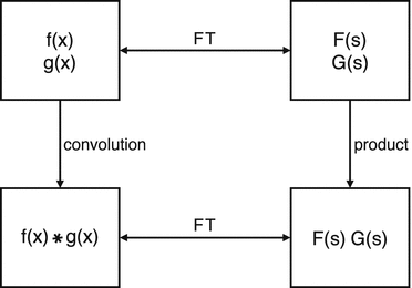

  

  Relationships involving Fourier transforms and convolution. As elsewhere in this book, the in-line asterisk indicates convolution.

• Correlation property. The correlation function is defined as

  $$\displaystyle{ r(y) =\int _{ -\infty }^{\infty }f(x)\,g(x - y)\,dx\;, }$$

  (A2.40)

  which can be written with the correlation operator, ⋆, as

  $$\displaystyle{ r(y) = f(x) \star g(x)\;. }$$

  (A2.41)

  The correlation property is

  $$\displaystyle{ f(x) \star g(x)\longleftrightarrow F(s)G^{{\ast}}(s)\;. }$$

  (A2.42)

  The Fourier transform of Eq. (A2.40) is

  $$\displaystyle{ R(s) =\int _{ -\infty }^{\infty }\left [\int _{ -\infty }^{\infty }f(x)\,g(x - y)\,dx\right ]\,e^{-j2\pi sy}dy\;. }$$

  (A2.43)

  Interchanging the order of integration and making the substitution z = x − y gives

  $$\displaystyle{ R(s) =\int _{ -\infty }^{\infty }f(x)\left [\int _{ -\infty }^{\infty }g(z)\,e^{\,j2\pi z}dz\right ]\,e^{-j2\pi sx}dx\;, }$$

  (A2.44)

  which results in

  $$\displaystyle{ R(s) = F(s)\,G^{{\ast}}(s)\;. }$$

  (A2.45)

  This relationship is shown in Fig. 8.1 An example where f(x) = g(x) = boxcar is shown in Fig. A2.3. Since f(x) is an even function, convolution and correlation are the same, both producing even functions. Hence, F(s) is real and even, and F(s)F(s) = F(s)F ^∗(s).

  Fig. A2.3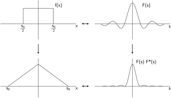

  

  Example of the correlation and convolution theorems for an even function f(x). The vertical arrow on the left indicates f ∗ f for the case of convolution and f ⋆ f for correlation. The vertical arrow on the right indicates F(s)F(s) for convolution and F(s)F ^∗(s) for correlation.

• Parseval’s theorem. The relationship

  $$\displaystyle{ \int _{-\infty }^{\infty }\vert \,f(x)\vert ^{2}dx =\int _{ -\infty }^{\infty }\vert F(s)\vert ^{2}ds }$$

  (A2.46)

  is known generally as Parseval’s theorem.⁵ To prove it, we write

  $$\displaystyle\begin{array}{rcl} \int _{-\infty }^{\infty }f(x)f^{{\ast}}(x)\,dx =\int _{ -\infty }^{\infty }{\Biggl [\,\int _{ -\infty }^{\infty }F(s)e^{\,j2\pi sx}ds\,\Biggr ]}\,{\Biggl [\int _{ -\infty }^{\infty }F^{{\ast}}(s')e^{-j2\pi s'x}ds'\,\Biggr ]}\,dx& & \\ & & {}\end{array}$$

  (A2.47)

  or

  $$\displaystyle{ \int _{-\infty }^{\infty }f(x)f^{{\ast}}(x)\,dx =\int _{ -\infty }^{\infty }\int _{ -\infty }^{\infty }F(s)F^{{\ast}}(s')\,{\Biggl [\int _{ -\infty }^{\infty }e^{\,j2\pi (s-s')x}dx\,\Biggr ]}\,ds\,ds'\;. }$$

  (A2.48)

  The integral in brackets is δ(s − s′), so that

  $$\displaystyle{ \int _{-\infty }^{\infty }f(x)f^{{\ast}}(x)\,dx =\int _{ -\infty }^{\infty }F(s)F^{{\ast}}(s)\,ds\;. }$$

  (A2.49)

  A useful theorem in interferometry is the projection–slice theorem, which is proved in Sect. 2.4.1.

2.1.3 A2.1.3 Two-Dimensional Fourier Transform

The two-dimensional Fourier transform between f(x, y) and F(u, v) can be written

$$\displaystyle{ \begin{array}{rl} F(u,v)& =\int _{ -\infty }^{\infty }\int _{-\infty }^{\infty }f(x,y)\,e^{-j2\pi (ux+vy)}dx\,dy\;, \\ f(x,y)& =\int _{ -\infty }^{\infty }\int _{-\infty }^{\infty }F(u,v)\,e^{\,j2\pi (ux+vy)}du\,dv\;. \end{array} }$$

(A2.50)

If x and y are in radians, then u and v are in units of cycles/radian. We write symbolically

$$\displaystyle{ f(x,y)\longleftrightarrow F(u,v)\;. }$$

(A2.51)

All of the properties in Appendix A2.1.2 have analogs in the two-dimensional Fourier transform. For example, the shift theorem is

$$\displaystyle{ f(x - x_{0},y - y_{0})\longleftrightarrow e^{-j2\pi (ux_{0}+vy_{0})}F(u,v)\;. }$$

(A2.52)

The two-dimensional Fourier transform can be converted to polar coordinates by defining x = rcosθ, y = rsinθ, u = qcosϕ, and v = qsinϕ, which leads to

$$\displaystyle{ F(q,\phi ) =\int _{ 0}^{2\pi }\int _{ 0}^{\infty }f(r,\theta )\,e^{-j2\pi rq(\theta -\phi )}r\,dr\,d\theta \;. }$$

(A2.53)

If f(r, θ) = f(r), i.e., f is azimuthally symmetric, then

$$\displaystyle{ F(q,\phi ) =\int _{ 0}^{\infty }f(r)\,r\,dr\int _{ 0}^{2\pi }e^{-j2\pi rq(\theta -\phi )}d\theta \;. }$$

(A2.54)

Since the zeroth-order Bessel function is defined as

$$\displaystyle{ J_{0}(z) = \frac{1} {2\pi }\int _{0}^{2\pi }e^{-jz\cos \theta }d\theta \;, }$$

(A2.55)

F(q, ϕ) = F(q) and

$$\displaystyle\begin{array}{rcl} F(q)& = 2\pi \int _{0}^{\infty }f(r)J_{0}(2\pi qr)r\,dr\;.&{}\end{array}$$

(A2.56a)

By symmetry,

$$\displaystyle\begin{array}{rcl} f(r)& = 2\pi \int _{0}^{\infty }F(q)J_{0}(2\pi qr)q\,dq\;.&{}\end{array}$$

(A2.56b)

Equations (A2.56a) and (A2.56b) are called the Hankel transform pair.

2.1.4 A2.1.4 Fourier Series

The Fourier series is a special case of the Fourier transform. A periodic function f(x), which repeats over the interval − x ₀∕2, x ₀∕2, has the complex Fourier series representation

$$\displaystyle{ f(x) =\sum \limits _{ -\infty }^{\infty }\alpha _{ k}\,e^{\frac{j2\pi kx} {x_{0}} }\;, }$$

(A2.57)

where

$$\displaystyle{ \alpha _{k} =\int _{ -\frac{x_{0}} {2} }^{ \frac{x_{0}} {2} }f(x)\,e^{-\frac{j2\pi kx} {x_{0}} }\,dx\;. }$$

(A2.58)

If we define f ₀(x) as f(x) over the interval − x ₀∕2, x ₀∕2, then its Fourier transform, F(s), is given by

$$\displaystyle{ F(s) =\sum _{ k=0}^{\infty }F_{ 0}(ks_{0})\,\delta (s - ks_{0})\;, }$$

(A2.59)

where s ₀ = 1∕x ₀ and F ₀(ks ₀) = α _k . This is called a line spectrum: F(s) consists of delta functions spaced at intervals s = 1∕x ₀ with amplitudes corresponding to the Fourier coefficients. Parseval’s theorem for the Fourier series can be found by substituting Eqs. (A2.57) and (A2.59) into Eq. (A2.49), yielding

$$\displaystyle{ \sum _{-\infty }^{\infty }\alpha _{ k}^{2} =\int _{ -\frac{x_{0}} {2} }^{ \frac{x_{0}} {2} }f(x)f^{{\ast}}(x)\,dx\;. }$$

(A2.60)

2.1.5 A2.1.5 Truncated Functions

The Fourier transform theory described above can be applied to functions that are random processes. If an ergodic random process has an associated temporal function f(x), that function generally extends to infinity, and ∫ | f(x) | ² = ∞, which presents certain theoretical difficulties. These difficulties are mitigated by choosing a truncated version of the function

$$\displaystyle{ f_{T}(x) = f(x)\varPi (x/x_{0})\;, }$$

(A2.61)

where Π(x) is the boxcar function defined after Eq. (A2.12). By the convolution property [Eq. (A2.35)],

$$\displaystyle{ F_{T}(s) = F(s) {\ast}\,\text{sinc}(sx_{0})\;. }$$

(A2.62)

Truncation has the effect of smoothing, or limiting the resolution of, F(s).

The power spectrum of a truncated function is usually defined as

$$\displaystyle{ P_{T}(s) = \frac{1} {T}F(s)\,F^{{\ast}}(s)\;, }$$

(A2.63)

which has units of power and does not depend on T. Note that the Fourier transform as defined for deterministic functions in previous sections is actually an energy density spectrum. The conditions under which the Fourier transform of an autocorrelation function and its power spectrum exist for random processes were first explored and clarified by Wiener and Khinchin. Hence, the Fourier transform between the autocorrelation function of a random process and its power spectrum is formally called the Wiener–Khinchin theorem (or relation).

References

Bracewell, R.N., Strip Integration in Radio Astronomy, Aust. J. Phys., 9, 198–217 (1956)
Bracewell, R.N., Radio Interferometry of Discrete Sources, Proc. IRE, 46, 97–105 (1958)
Bracewell, R.N., Two-Dimensional Imaging, Prentice-Hall, Englewood Cliffs, NJ (1995)
Bracewell, R.N., The Fourier Transform and Its Applications, McGraw-Hill, New York (2000) (earlier eds. 1965, 1978)
Bracewell, R.N., and Riddle, A.C., Inversion of Fan Beam Scans in Radio Astronomy, Astrophys. J., 150, 427–434 (1967)
Bracewell, R.N., and Roberts, J.A., Aerial Smoothing in Radio Astronomy, Aust. J. Phys., 7, 615–640 (1954)
Champeney, D.C., Fourier Transforms and Their Physical Applications, Academic Press, London (1973)
de Pater, I., and Sault, R.J., An Intercomparison of Three-Dimensional Reconstruction Techniques Using Data and Models of Jupiter’s Synchrotron Radiation, J. Geophys. Res., 103, 19973–19984 (1998)
de Pater, I., van der Tak, F., Strom, R.G., and Brecht, S.H., The Evolution of Jupiter’s Radiation Belts after the Impact of Comet D/Shoemaker–Levy 9, Icarus, 129, 21–47 (1997)
Papoulis, A., The Fourier Integral and Its Applications, McGraw-Hill, New York (1962)
Sault, R.J., Oosterloo, T., Dulk, G.A., and Leblanc, Y., The First Three-Dimensional Reconstruction of a Celestial Object at Radio Wavelengths: Jupiter’s Radiation Belts, Astron. Astrophys., 324, 1190–1196 (1997)
Author information
Authors and Affiliations