Homogeneous Deformation of Multi-Agent Systems Communication

Abstract

In this chapter, it is shown how a multi-agent system (MAS) can acquire a desired homogeneous deformation in $\mathbb{R}^{n}$ (prescribed by n + 1 leaders) through local communication. For this purpose, two communication protocols are developed. The first protocol, that is called minimum communication, allows each follower to communicate only with n + 1 local agents. Under this protocol, communication weights

These keywords were added by machine and not by the authors. This process is experimental and the keywords may be updated as the learning algorithm improves.

In this chapter, it is shown how a multi-agent system (MAS) can acquire a desired homogeneous deformation in $\mathbb{R}^{n}$ (prescribed by n + 1 leaders) through local communication. For this purpose, two communication protocols are developed. The first protocol, that is called minimum communication, allows each follower to communicate only with n + 1 local agents. Under this protocol, communication weights are uniquely determined based on the initial positions of a follower i and n + 1 agents that are adjacent to the follower i. Followers apply first order linear dynamics to acquire the desired position defined by a homogeneous transformation. The second protocol, that is called preservation of volumetric ratios, permits followers to interact with more than n + 1 local agents. Under this setup, local volumetric ratios are obtained based on the initial positions of a follower i and m _i  ≥ n + 1 agents that are adjacent to the follower i. Then each follower applies a nonlinear dynamics to acquire the desired position (prescribed by a homogeneous mapping) through keeping transient volumetric ratios, specified based on current positions of the agents, as close as initial values of the volumetric ratios.

3.1 Graph Theory Notions and Definitions

Basic Notions: For an MAS moving in $\mathbb{R}^{n}$ (n denotes dimension of the motion field; n can be either 1, 2, or 3.), interagent communication is prescribed by a directed graph (digraph) G = (V _G , E _G ), where V _G  = { 1,  2, …,  N} and E _G  ∈ V _G × V _G are sets of nodes and edges of the graph. The state (position and velocity) of the node i can be accessed by the node j, if (i, j) ∈ E _G . The set N _i  = { j: (j, i) ∈ E _G } is called the in-neighbor set of the vertex i, where d _i  = | N _i  | is the cardinality of N _i . A graph is called undirected, if communication between every two connected nodes of the graph is bidirectional. (If (j, i) ∈ E _G , then (i, j) ∈ E _G .) A finite (or infinite) sequence of edges which connects a finite sequence of vertices is called a path. An undirected graph is connected, if there exists at least a path between any two nodes of an undirected graph. A directed graph is called weakly connected, if substituting every directed edge by an undirected edge yields a connected undirected graph. Two vertices i and j in the digraph G are called connected, if there exists a directed path from i to j, and one from j to i. A digraph G is called strongly connected, if every two nodes of G is connected. A graph G defining interagent communication can be expressed by the independent sum

$$\displaystyle{G =\phi \oplus \partial \phi,}$$

where the ∂ ϕ is the boundary graph representing boundary nodes of G and the subgraph ϕ represents interior nodes of G.

Definition 1.

An agent i is called a leader, if the in-neighbor set N _i is empty. This implies that leaders move independently. Leaders are identified by the numbers 1,  2, …,  N _l (N _l  ≤ N). The leader set

$$\displaystyle{V _{L} =\{ 1,\ 2,\ldots,\ N_{l}\}}$$

defines index numbers of leaders.

Definition 2.

An agent i is called a follower, if the in-neighbor set N _i is nonempty. In other words, every follower agent can access state information (position and velocity) of the in-neighbor agents. Followers are identified by the numbers N _l + 1,  N _l + 2, …,  N. The follower set

$$\displaystyle{V _{F} =\{ N_{l} + 1,\ N_{l} + 2,\ldots,\ N\}}$$

defines index numbers of followers.

Definition 3.

The set $C \subset \mathbb{R}^{n}$ is convex, if for every x and y in C, then (1 −α)x +α y is in C for all α ∈ [0, 1].

Definition 4.

Let $R =\{ r_{1},\ r_{2},\ldots,\ r_{N_{l}}\}$ specify a set of vectors in $\in \mathbb{R}^{n}$, then intersections of convex sets containing R is called a convex hull. Mathematically speaking,

$$\displaystyle{ Conv(R) =\{ r_{i} =\sum _{ j=1}^{N_{l} }\alpha _{i,j},r_{j} \in \mathbb{R}^{n}\vert \alpha _{ i,j} \geq 0 \wedge \sum _{j=1}^{N}\alpha _{ i,j} = 1\}. }$$

(3.1)

3.2 Protocol of Minimum Communication

Consider a communication graph G = ϕ ⊕ ∂ ϕ with n + 1 nodes belonging to the boundary graph ∂ ϕ and N − n − 1 nodes belonging to the subgraph ϕ. The nodes belonging to the subgraph ϕ and the boundary graph ∂ ϕ represent followers and leaders, respectively. Notice that leaders move independently, but position of each leader is tracked by a follower. Therefore, follower-leader communication is unidirectional and shown by an arrow terminated to the follower. Communication between two follower agents can be either unidirectional or bidirectional. This implies that the subgraph ϕ is directed. It is noted that communication weights are not inevitably the same for the two connected nodes in ϕ. Also, any node belonging to the subgraph ϕ can access state information of n + 1 in-neighbor agents. A typical communication graph for an MAS evolving in a plane ($\in \mathbb{R}^{2}$) is shown in Fig. 3.1. As it is seen in Fig. 3.1, the MAS consists of 20 agents (3 leaders and 17 followers), where each follower interacts with 3 local agents, and communication between two in-neighbor followers is bidirectional.

Fig. 3.1

An interagent communication graph used for MAS evolution in a plane ($\in \mathbb{R}^{2}$)

Next, it is described how communication weights can be uniquely determined based on the initial positions of the agents.

3.2.1 Communication Weights

Let the follower i ∈ V _F access positions of n + 1 agents i ₁,  i ₂, …,  i _n+1 belonging to the in-neighbor set N _i . Suppose that agents i, i ₁, i ₂, …, i _n+1 are initially positioned at R _i , $R_{i_{1}}$, $R_{i_{2}}$, …, $R_{i_{n+1}}$, respectively. It is assumed that

$$\displaystyle{ Rank\left [\begin{array}{*{10}c} R_{i_{2}} - R_{i_{1}} & \ldots & R_{i_{n+1}} - R_{i_{1}} \end{array} \right ] = n. }$$

(3.2)

Then R _i can be uniquely expanded as follows:

$$\displaystyle{ R_{i} = R_{i_{1}} +\sum _{ j=2}^{n+1}w_{ i,i_{j}}(R_{i_{j}} - R_{i_{1}}) = (1 -\sum _{j=2}^{n+1}w_{ i,i_{j}})R_{i_{1}} +\sum _{ j=2}^{n+1}w_{ i,i_{j}}R_{i_{j}}. }$$

(3.3)

Let

$$\displaystyle{ w_{i,i_{1}} = 1 -\sum _{j=2}^{n+1}w_{ i,i_{j}}, }$$

(3.4)

then

$$\displaystyle{ R_{i} =\sum _{ j=1}^{n+1}w_{ i,i_{j}}R_{i_{j}}. }$$

(3.5)

By considering Eq. (3.4), and Eq. (3.5) written in the component wise form, the parameter $w_{i,i_{j}}$ is uniquely determined by solving the following set of n + 1 linear algebraic equations:

$$\displaystyle{ \left [\begin{array}{*{10}c} X_{1,i_{1}} & X_{1,i_{2}} & \ldots & X_{1,i_{n+1}} \\ X_{2,i_{1}} & X_{2,i_{2}} & \ldots & X_{2,i_{n+1}}\\ \vdots & \vdots & & \vdots \\ X_{n,i_{1}} & X_{n,i_{2}} & \ldots & X_{n,i_{n+1}} \\ 1 & 1 & & 1\\ \end{array} \right ]\left [\begin{array}{*{10}c} w_{i,i_{1}} \\ w_{i,i_{2}}\\ \vdots \\ w_{i,i_{n}} \\ w_{i,i_{n+1}}\\ \end{array} \right ] = \left [\begin{array}{*{10}c} X_{1,i} \\ X_{2,i}\\ \vdots \\ X_{n,i} \\ 1 \end{array} \right ]. }$$

(3.6)

It is noted that X _q, h is the q ^th component of the initial position of the agent h ∈ { i,  i ₁, …,  i _n+1}. The communication weights are all positive, if the follower i ∈ V _F is initially located inside the communication polytope whose vertices are occupied by the agents i ₁, …, i _n+1.

MAS evolution in a plane: If an MAS evolves in a plane, then homogeneous deformation is prescribed by three leaders at the vertices of the leading triangle; desired position of a follower i is specified by Eq. (2.17) as a convex combination of positions of three leaders. Follower i interacts with three agents i ₁, i ₂, and i ₃ to acquire the desired position through local communication. As shown in Fig. 3.2, the motion plane is divided into seven subregions based on the signs of the communication weights. It is evident that communication weights $w_{i,i_{1}}$, $w_{i,i_{2}}$, and $w_{i,i_{3}}$ are all positive, if the follower i is initially placed inside the communication triangle whose vertices are occupied by the adjacent agents i ₁, i ₂, and i ₃.

Fig. 3.2

Dividing motion plane into seven sub-regions based on the signs of communication weights

For MAS evolution in the X − Y plane, communication weights simplify to

$$\displaystyle{ \left [\begin{array}{*{10}c} X_{i_{1}} & X_{i_{2}} & X_{i_{3}} \\ Y _{i_{1}} & Y _{i_{2}} & Y _{i_{3}} \\ 1 & 1 & 1\\ \end{array} \right ]\left [\begin{array}{*{10}c} w_{i,i_{1}} \\ w_{i,i_{2}} \\ w_{i,i_{3}}\\ \end{array} \right ] = \left [\begin{array}{*{10}c} X_{i} \\ Y _{i} \\ 1\\ \end{array} \right ]. }$$

(3.7)

where the first and second components of the initial position of the agent h ∈ { i,  i ₁,  i ₂,  i ₃} are denoted by X _h and Y _h , respectively. In Table 3.1, positions of agents in the initial formation, shown in Fig. 3.1, and the corresponding communication weights are listed.

Table 3.1 Initial positions and communication weights associated with the formation shown in Fig. 3.1

Remark 3.1.

It is noticed that the total number of the agents is even, when an MAS is supposed to evolve in a plane and the minimum interagent communication is issued by a connected (and undirected) graph. This is because the MAS consists of 3 leaders, and each follower is restricted to interact with three local agents, where follower-follower communication is bidirectional.

3.2.2 Weight Matrix

Let the weight matrix $W \in \mathbb{R}^{(N-n-1)\times (N-n-1)}$ be defined as follows:

$$\displaystyle{ W_{ji} = \left \{\begin{array}{@{}l@{\quad }l@{}} w_{i+n+1,j}> 0\quad &if(j,i + n + 1) \in E_{G} \\ -1 \quad &i + n + 1 = j \\ 0, \quad &else \end{array} \right.. }$$

(3.8)

Then matrix W has the following properties:

• Each row of the matrix W has n + 2 nonzero entries.

• Sum of every row of the matrix W is zero.

If the matrix W is partitioned as follows:

$$\displaystyle{ W = \left [\begin{array}{*{10}c} B \in \mathbb{R}^{(N-n-1)\times (n+1)} & A \in \mathbb{R}^{(N-n-1)\times (N-n-1)}\\ \end{array} \right ], }$$

(3.9)

then every column of the matrix B has only one positive entry, while the remaining entries of B are all zero. Even if follower-follower communication is bidirectional, the matrix A is not necessarily symmetric; however, if A _ij  = 0, then A _ji  = 0, and if A _ij ≠ 0, then A _ji ≠ 0.

In the following theorem, it is proven that the matrix A = −(I − F) is Hurwitz, if the matrix $F \in \mathbb{R}^{(N-n-1)\times (N-n-1)}$ is nonnegative and irreducible.

Theorem 3.1.

For MAS evolution in $\mathbb{R}^{n}$ , if (i) interagent communication is defined by a digraph G = ϕ ⊕ ∂ϕ with directed and strongly connected subgraph ϕ, and (ii) communication weights, determined by Eq.  (3.6) , are all positive, then the matrix A is Hurwitz.

Proof.

The matrix A = −(I − F) is obtained by eliminating the first n + 1 columns from the matrix W. Since W is zero-sum row, sum of each of the first n + 1 rows of A is negative, and the remaining rows of A are zero-sum. In other words, sum of each of the first n + 1 rows of the nonnegative and irreducible matrix F is less than 1, while the remaining rows of F are one-sum. By provoking Perron-Frobenius theorem [102], it is concluded that the spectrum of the matrix F, which is denoted by ρ(F), is not greater than 1. However, A is a non-singular M-matrix [9]. This is because sum of each of the first n + 1 rows of the matrix A is negative. Therefore, the spectrum of the matrix F cannot be equal to 1 and the matrix A is necessarily Hurwitz.

Remark 3.2.

It is not necessarily required that all communication weights are positive in order to assure achieving homogeneous transformation under local communication. In fact, positiveness of communication weights is a sufficient condition. For instance, initial distribution of an MAS shown in Fig. 3.3 results in two positive communication weights w _11, 10 and w _11, 14 and a negative weight w _11, 13. However, the partition A of the weight matrix W that is consistent with the initial positions of agents is still Hurwitz. This guarantees that positions of followers asymptotically converge to desired positions in the ultimate formation, where final formation is a homogeneous transformation of the initial configuration.

Fig. 3.3

An initial distribution of agents resulting in negative weights of communication for some followers

Desired Positions of Followers Issued by a Homogeneous Deformation: Let

$$\displaystyle{Z_{q} = \left [\begin{array}{*{10}c} X_{q,n+2} & \ldots & X_{q,N} \end{array} \right ]^{T} \in \mathbb{R}^{N-n-1}}$$

and

$$\displaystyle{U_{q} = \left [\begin{array}{*{10}c} X_{q,1} & \ldots & X_{q,n+1} \end{array} \right ]^{T} \in \mathbb{R}^{n+1}}$$

denote the q ^th components of the initial positions of the followers and leaders, respectively, then

$$\displaystyle{ AZ_{q} + BU_{q} = 0. }$$

(3.10)

This represents consistency between communication weights and initial positions of the agents (See Eq. (3.6).) Notice that the q ^th component of Eq. (3.3) is the same as the row i − n − 1 of Eq. (3.10). Because A is Hurwitz, the q ^th components of positions of followers are determined by

$$\displaystyle{ Z_{q} = -A^{-1}BU_{ q}. }$$

(3.11)

The row i of Eq. (3.11) is equal to

$$\displaystyle{ X_{q,i+n+1} =\sum _{ k=1}^{n+1}\alpha _{ i+n+1,k}X_{q,k}(t), }$$

(3.12)

where X _q, i (the q ^th component of the position of the follower i ∈ V _F ) is expressed as the linear combination of the q ^th components of positions of leaders. It is noted that the parameter α _i+n+1, k is uniquely obtained from Eq. (2.15), if initial positions of leaders satisfy the rank condition (2.3). Therefore, the ik entry of the matrix

$$\displaystyle{ W_{L} = -A^{-1}B \in \mathbb{R}^{(N-n-1)\times (n+1)}. }$$

(3.13)

is inevitably equal to α _i+n+1, k .

The desired position of the follower i, satisfying the condition of a homogeneous transformation, is specified by Eq. (2.14). Let

$$\displaystyle{ x_{q,i+n+1,HT} =\sum _{ k=1}^{n+1}\alpha _{ i+n+1,k}x_{q,k}(t),\ (i + n + 1) \in V _{F}, }$$

(3.14)

be the q ^th component of r _i+n+1, HT , then

$$\displaystyle{z_{q,HT}(t) = \left [\begin{array}{*{10}c} x_{q,n+2,HT}&\ldots &x_{q,N,HT} \end{array} \right ]^{T} \in \mathbb{R}^{N-n-1}}$$

defines the q ^th components of the desired positions of followers. Given u _q (t) (the q ^th components of the leaders’ positions at a time t), then

$$\displaystyle{ z_{q,HT}(t) = W_{L}u_{q}(t). }$$

(3.15)

Remark 3.3.

If communication weights are all positive, then Eq. (3.15) assures that every follower is initially placed inside the i ^th communication polytope whose vertices are occupied by the agents i ₁, i ₂, …, i _n+1. However, an arbitrary initial distribution of agents may not necessarily result in positive communication weights (See Remark 3.2.) In order to guarantee that positive communication weights are consistent with agents’ positions, initial positions of the followers can be determined by applying the following procedure:

• A communication graph G satisfying the properties specified in Section 3.1 is considered.

• Given the communication graph G, n + 1 arbitrary positive weights $w_{i,i_{1}}$, $w_{i,i_{2}}$, …, $w_{i,i_{n+1}}$ are considered for communication between the follower i and n + 1 in-neighbor agents i ₁, i ₂, …, i _n+1 such that

  $$\displaystyle{ \sum _{k=1}^{n+1}w_{ i,i_{k}} = 1,\ \forall \ i \in V _{F}. }$$

  (3.16)

• The weight matrix $W \in \mathbb{R}^{(N-n-1)\times N}$ is set up by using the relation (3.8), and then partitions $B \in \mathbb{R}^{(N-n-1)\times (n+1)}$ and $A \in \mathbb{R}^{(N-n-1)\times (N-n-1)}$ of W are determined.

• Leaders are positioned at R ₁, R ₂, …, R _n+1 at the initial time t ₀, where leaders’ initial positions satisfy the rank condition (2.3).

• The q ^th components of the initial positions of followers are assigned by using Eq. (3.11).

Example 3.1.

Let the graph shown in Fig. 3.4 define communication among agents of an MAS containing 3 leaders and 7 followers. The boundary nodes 1, 2, and 3 represent leaders, and the interior nodes 4, 5, …, 10 represent followers. As it is seen, each follower interacts with three local agents, where follower-follower communication is bidirectional.

Fig. 3.4

A typical communication graph used for MAS evolution in a plane ($\in \mathbb{R}^{2}$)

Weights listed in Table 3.2 are considered for inter-agent communications among the agents. Notice that sum of the communication weights of each follower is equal to 1 ($w_{i,i_{1}} + w_{i,i_{2}} + w_{i,i_{3}} = 1,\ \forall i \in V _{F}$). By using the definition (3.8), the weight matrix $W \in \mathbb{R}^{7\times 10}$ is obtained as follows:

$$\displaystyle{ W = \left [\begin{array}{*{10}c} 0.70& 0 & 0 & -1 & 0 & 0 &0.15& 0 & 0 &0.15\\ 0 &0.70 & 0 & 0 & -1 & 0 & 0 &0.15 &0.15 & 0 \\ 0 & 0 &0.70& 0 & 0 & -1 & 0 & 0 &0.15&0.15\\ 0 & 0 & 0 &0.40 & 0 & 0 & -1 &0.36 & 0 &0.24 \\ 0 & 0 & 0 & 0 & 1/3 & 0 & 1/3 & -1 & 1/3 & 0 \\ 0 & 0 & 0 & 0 &0.31&0.42& 0 &0.27& -1 & 0\\ 0 & 0 & 0 &0.35 & 0 &0.29 &0.36 & 0 & 0 & -1 \\ \end{array} \right ]. }$$

(3.17)

Table 3.2 Communication weights associated with the formation shown in Fig. 3.4

Leader agents are placed at (X ₁, Y ₁) = (−6. 5, −6. 5), (X ₂, Y ₂) = (−5. 5, 6), and (X ₃, Y ₃) = (6, 5) at the initial time. Note that initial positions of leaders satisfy the rank condition (2.3). Initial positions of the followers are obtained by using Eq. (3.11) as listed in Table 3.3. Additionally, parameters α _i, k ($\forall i \in V _{F},\ k \in V _{L}$) are calculated by using Eq. (2.19) and listed in the last three columns of Table 3.3.

Table 3.3 Initial positions of agents; parameters α _i, 1,  α _i, 2,  α _i, 3 for the follower agent i

3.2.3 MAS Evolution Dynamics-First Order Kinematic Model-Method 1

Let position of the agent i ∈ V be updated by

$$\displaystyle{ \dot{r}_{i}(t) = u_{i} }$$

(3.18)

where

$$\displaystyle{ u_{i} = \left \{\begin{array}{@{}l@{\quad }l@{}} Given \quad &\ i \in V _{L} \\ -g_{i}r_{i}(t - h{_{1}}_{i}) + g_{i}r_{i,d}(t - h{_{2}}_{i}) +\beta \dot{ r}_{i,d}(t - h{_{2}}_{i})\quad &i \in V _{F} \end{array} \right.. }$$

(3.19)

It is noted that leaders move independently, therefore their positions are known at any time t. Also,

$$\displaystyle{ r_{i,d}(t) =\sum _{j\in N_{i}}w_{i,j}r_{j}(t) }$$

(3.20)

where w _i, j is the communication weight, $g_{i} \in \mathbb{R}_{+}$ is constant, and h _{1 i}  ≥ 0 and h _{2 i}  ≥ 0 are constant time delays. If h _{1 i}  = 0, the follower i can immediately access its own position (without time delay) at any time t. If h _{2 i}  = 0, follower i accesses positions of its in-neighbor agents (belonging to the set N _i ) without communication delay. The parameter β can be either 0 or 1. If β = 0, then position of the follower i is updated based on the positions of the neighboring agents. If β = 1, then position of the follower i is updated based on both positions and velocities of the neighboring agents. Evolution of an MAS in absence/presence of communication delays is studied in the subsections 3.2.3.1 and 3.2.3.2.

3.2.3.1 Evolution of Followers in Absence of Communication Delays

Followers without Body Size

Let h _{1 i} and h _{2 i} in Eqs. (3.18) and (3.19) be both zero, then position of the follower i ∈ V _F is updated by

$$\displaystyle{ \dot{r}_{i} = g_{i}(r_{i,d}(t) - r_{i}(t)). }$$

(3.21)

Suppose that $z_{q} = [x_{q,n+2}\ \ldots \ x_{q,N}]^{T} \in \mathbb{R}^{N-n-1}$ defines the q ^th components of the positions of followers at the time t, then z _q is updated by the following first order matrix dynamics:

$$\displaystyle{ \dot{z}_{q} = G(Az_{q} + Bu_{q}). }$$

(3.22)

It is noticed that Eq. (3.21) and the row i − n − 1 of the MAS evolution dynamics given by Eq. (3.22) are identical, and

$$\displaystyle{ G = diag(g_{n+2},\ g_{n+3},\ldots,\ g_{N}) \in \mathbb{R}^{(N-n-1)\times (N-n-1)} }$$

(3.23)

is a positive diagonal matrix. Because the matrix A is Hurwitz, the dynamics of Eq. (3.22) is stable and z _q asymptotically converges to

$$\displaystyle{ Z_{F,q} = W_{L}U_{F,q} = -A^{-1}BU_{ F,q}, }$$

(3.24)

where U _F, q specifies the q ^th components of final positions of leaders. Because the ik entry of the matrix W _L is equal to α _i+n+1, k (α _i+n+1, k is uniquely determined by Eq. (2.15) based on the initial positions of the follower i + n + 1 and n + 1 leaders), final position of the follower i satisfies Eq. (3.14). Therefore, final formation of the MAS is a homogeneous deformation of the initial configuration.

Example 3.2.

It is assumed that an MAS, consisting of 20 agents (3 leaders and 17 followers), negotiates a narrow channel in the X − Y plane. Initial and final formations P and Q are shown in Fig. 3.5. Notice that the formation Q is a homogeneous transformation of the initial MAS configuration P, where initial positions of the agents are listed in Table 3.1. Also, final positions of the agents are listed in the last two columns of Table 3.1.

Fig. 3.5

Initial and desired final configurations of an MAS negotiating a narrow channel

Positions of the leaders are defined by

$$\displaystyle\begin{array}{rcl} Leader\;1: \left \{\begin{array}{@{}l@{\quad }l@{}} x_{1}(t) = -6.5 + \dfrac{12.5} {30} t\quad &t \leq 30 \\ x_{1}(t) = 6 \quad &t> 30 \\ y_{1}(t) = -6.5 + \dfrac{18} {30}t \quad &t \leq 30 \\ y_{1}(t) = 11.5 \quad &t> 30\\ \quad \end{array} \right.& &{}\end{array}$$

(3.25)

$$\displaystyle\begin{array}{rcl} Leader\;2: \left \{\begin{array}{@{}l@{\quad }l@{}} x_{2}(t) = -5.5 + 5.5\cos ( \dfrac{\pi t} {60} + \dfrac{3\pi } {2})\quad &t \leq 30 \\ x_{2}(t) = 0 \quad &t> 30 \\ y_{2}(t) = 11.5 + 5.5\sin ( \dfrac{\pi t} {60} + \dfrac{3\pi } {2}) \quad &t \leq 30 \\ y_{2}(t) = 11.5 \quad &t> 30\\ \quad \end{array} \right.& &{}\end{array}$$

(3.26)

$$\displaystyle\begin{array}{rcl} Leader\;3: \left \{\begin{array}{@{}l@{\quad }l@{}} x_{3}(t) = 6\dfrac{12.5} {30} t \quad &t \leq 30 \\ x_{3}(t) = 6 \quad &t> 30 \\ y_{3}(t) = 5.5 + \dfrac{10.5} {30} t\quad &t \leq 30 \\ y_{3}(t) = 16 \quad &t> 30\\ \quad \end{array} \right.& &{}\end{array}$$

(3.27)

In Fig. 3.6, paths chosen by the three leaders (at the vertices of the leading triangle) are depicted.

Fig. 3.6

Paths of the leaders in example 3.2

Homogeneous transformation of the MAS is related to the trajectories chosen by the three leaders placed at the vertices of the leading triangle. Entries of the Jacobian matrix $Q \in \mathbb{R}^{2\times 2}$ and rigid body displacement vector $D \in \mathbb{R}^{2}$, that are specified based on the first (X) and second (Y ) components of the positions of leaders, are shown versus time in Fig. 3.7. As it is observed, $Q(0) = I \in \mathbb{R}^{2\times 2}$ and $D(0) = 0 \in \mathbb{R}^{2}$. Therefore, r _i (0) = R _i ($\forall i \in V$).

Fig. 3.7

Entries Q and D versus time

Each follower updates its current position according to Eq. (3.21), where g _i  = g = 30 ($\forall i \in V _{F}$), and the communication weights are consistent with the initial positions shown in Fig. 3.1 as listed in Table 3.1. The X and Y components of the desired and actual positions of the follower 18 are depicted versus time in Fig. 3.8. As it is seen in Fig. 3.8, follower 18 deviates from its desired position during transition, however, it ultimately reaches the final desired position, (X _F, 18, Y _F, 18) = (3. 3437, 12. 7074).

Fig. 3.8

X and Y components of the desired and actual positions of the follower 18

Parameters p _18, 1, p _18, 2, and p _18, 3, calculated by using Eq. (2.13) based on the final positions of the follower 18 and the, are as follows:

$$\displaystyle{\left [\begin{array}{*{10}c} p_{18,1} \\ p_{18,2} \\ p_{18,3}\\ \end{array} \right ] = \left [\begin{array}{*{10}c} X_{1,F}&X_{2,F}&X_{3,F} \\ Y _{1,F} & Y _{2,F} & Y _{3,F} \\ 1 & 1 & 1\\ \end{array} \right ]^{-1}\left [\begin{array}{*{10}c} X_{18,F} \\ Y _{18,F} \\ 1\\ \end{array} \right ] = \left [\begin{array}{*{10}c} 6 & 0 & 6\\ 11.5 &11.5 &16 \\ 1 & 1 & 1 \end{array} \right ]^{-1}\left [\begin{array}{*{10}c} 3.3437\\ 12.7074 \\ 1 \end{array} \right ] = \left [\begin{array}{*{10}c} 0.2890\\ 0.4427 \\ 0.2683\\ \end{array} \right ].}$$

As it is observed, the ultimate values of p _18, 1, p _18, 2, p _18, 3 are the same as α _18, 1, α _18, 2, and α _18, 3 which are uniquely determined based on the initial positions of the follower 18 and the three leaders as follows:

$$\displaystyle{\left [\begin{array}{*{10}c} \alpha _{18,1} \\ \alpha _{18,2} \\ \alpha _{18,3}\\ \end{array} \right ] = \left [\begin{array}{*{10}c} X_{1} & X_{2} & X_{3} \\ Y _{1} & Y _{2} & Y _{3} \\ 1 & 1 & 1\\ \end{array} \right ]^{-1}\left [\begin{array}{*{10}c} X_{18} \\ Y _{18} \\ 1\\ \end{array} \right ] = \left [\begin{array}{*{10}c} -6.5&-5.5&6\\ -6.5 & 6 &5 \\ 1 & 1 &1 \end{array} \right ]^{-1}\left [\begin{array}{*{10}c} -2.6927\\ 2.1270 \\ 1 \end{array} \right ] = \left [\begin{array}{*{10}c} 0.2883\\ 0.4425 \\ 0.2692 \end{array} \right ].}$$

This implies that final formation of the MAS is a homogeneous transformation of the initial configuration.

Formations of the MAS at six sample times t = 5s, t = 10s, t = 15s, t = 20s, t = 25s, and t = 35s are shown in Fig. 3.9.

Fig. 3.9

MAS formations at five different sample times t = 5s, t = 10s, t = 15s, t = 20s, t = 25s, and t = 35s

Followers with Finite Body Size

As observed above, followers deviate from the desired positions defined by a homogeneous deformation during transition, when position of the follower i ∈ V _F is updated according to the first order dynamics (3.21). In this section, it is desired to specify an upper bound for the deviations of followers. Therefore, avoidance of interagent collision can be assured, when each follower has a finite size.

Constraints on leaders’ motion: The following four constraints are considered for motion of the leaders:

• Positions of leaders are required to satisfy the rank condition (2.3) at any time t. This condition assures that eigenvalues of the Jacobian matrix Q(t) remain positive at any time t, and thus the deformation mapping remains nonsingular.

• Paths of the leaders are chosen such that the leading polytope does not collide with obstacles in the motion field. A schematic of path planning, illustrating avoidance of collision of the leading triangle in the motion plane, is shown in Fig. 3.10.

  Fig. 3.10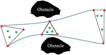

  

  Schematic of paths chosen by leaders assuring avoidance of agents with obstacle

• It is required that n + 1 leaders choose their trajectories such that desired positions of no two followers get closer than 2(δ +ε),

  $$\displaystyle{ i,j \in V \wedge i\neq j,\vert \vert r_{i,HT}(t) - r_{j,HT}(t)\vert \vert \geq 2(\delta +\epsilon ). }$$

  (3.28)

  Note that

  $$\displaystyle{ \delta \geq \vert \vert r_{i}(t) - r_{i,HT}(t)\vert \vert }$$

  (3.29)

  is the upper limit for deviation of follower agent i ∈ V _F form the desired position r _i, HT (t) given by a homogeneous deformation (δ is obtained in the sequel.). When each follower acquires homogeneous deformation through local communication.

• It is also necessary that distance of each follower from boundary of the leading polytope remains equal or greater than (δ +ε). This requirement guarantees that no follower leaves the leading polytope.

It is supposed that f ₁ ∈ V and f ₂ ∈ V are index numbers of two agents that have minimum separation distance

$$\displaystyle{ \gamma _{I} = \vert \vert R_{f_{1}} - R_{f_{2}}\vert \vert }$$

(3.30)

in the initial formation; γ _s is the minimum distance of a follower from the boundary of the leading polytope in the initial formation of the MAS. Graphical representations of γ _I and γ _s are shown in Fig. 3.11 for a typical initial distribution of agents in the X − Y plane.

Fig. 3.11

Graphical representations of γ _I and γ _s

Theorem 3.2.

Suppose that $\lambda _{min} \in \mathbb{R}_{+}$ is the lower limit for the magnitudes of eigenvalues of the matrix $\sqrt{Q^{T } Q} \in \mathbb{R}^{n\times n}$ ,

$$\displaystyle{\forall t \geq t_{0},\ \lambda _{min} \leq \lambda _{1}(\sqrt{Q^{T } Q}) <\ldots <\lambda _{n}(\sqrt{Q^{T } Q}).}$$

Also, assume that

$$\displaystyle{\gamma _{ij}(t) = \vert \vert r_{i,HT}(t) - r_{j,HT}(t)\vert \vert }$$

is the distance between two arbitrary agents i and j initially positioned at R _i and R _j , respectively. Then

$$\displaystyle{ \dfrac{\gamma _{ij}(t)} {\gamma _{ij}(t_{0})} = \dfrac{\vert \vert r_{i,HT}(t) - r_{j,HT}(t)\vert \vert } {\vert \vert R_{i} - R_{j}\vert \vert } \geq \lambda _{min}, }$$

(3.31)

if the leading polytope is deformed as a homogeneous transformation. Notice that t ₀ is the initial time and γ _ij (t ₀ ) = ||R _i − R _j ||.

Proof.

Under homogeneous deformation of a leading polytope, distance between two arbitrary agents i and j satisfies

$$\displaystyle{ r_{i,HT}(t) - r_{j,HT}(t) = Q(t)(R_{i} - R_{j}). }$$

(3.32)

By using polar decomposition [64], Q = R _O U _D , where R _O is orthogonal and U _D is a symmetric pure deformation matrix. So,

$$\displaystyle{ Q^{T}Q = U_{ D}^{T}U_{ D} }$$

(3.33)

and

$$\displaystyle{ \lambda (U_{D}) =\lambda (\sqrt{Q^{T } Q}). }$$

(3.34)

By considering definition of the homogeneous transformation,

$$\displaystyle{ r_{i,HT}(t) - r_{j,HT}(t) = Q(t)(R_{i} - R_{j}), }$$

(3.35)

therefore,

$$\displaystyle{ \begin{array}{r} (r_{i,HT}(t) - r_{j,HT}(t))^{T}(r_{i,HT}(t) - r_{j,HT}(t)) = (R_{i} - R_{j})^{T}Q^{T}Q(R_{i} - R_{j}) \geq \\ (R_{i} - R_{j})^{T}\lambda _{min}^{2}(R_{i} - R_{j}). \end{array} }$$

(3.36)

Consequently,

$$\displaystyle{ \lambda _{min} \leq \dfrac{\vert \vert r_{i,HT}(t) - r_{j,HT}(t)\vert \vert } {\vert \vert R_{i} - R_{j}\vert \vert } = \dfrac{\gamma _{ij}(t)} {\gamma _{ij}(t_{0})}. }$$

(3.37)

Remark 3.4.

Given ε (the radius of each follower), γ _I (initial distance between the agents f ₁ ∈ V and f ₂ ∈ V that are at the closest distance in the initial configuration) and γ _s (smallest distance of an agent from the boundary of the leading polytope), then

$$\displaystyle{ \delta _{max} = min\{\dfrac{1} {2}(\gamma _{I} - 2\epsilon ),(\gamma _{s}-\epsilon )\}. }$$

(3.38)

Note that no two followers get closer than 2(δ +ε) and no follower leaves the leading polytope, if

$$\displaystyle{ \lambda _{min} \leq \dfrac{2(\delta +\epsilon )} {2(\delta _{max}+\epsilon )}. }$$

(3.39)

It is noticed that δ is the upper limit for deviations of followers from the state of homogeneous transformation, when followers learn homogeneous deformation by local communication. Because entries of Q and D can be uniquely related to the components of leaders’ positions by using Eq. (2.8), it is necessary that trajectories of leaders are specified such that the minimum value of the smallest eigenvalues of the matrix $\sqrt{ Q^{T}Q}$ never becomes less than λ _min given by Eq. (3.39).

Upper Bound δ for Followers’ Deviations: Let dynamics of evolution of followers be expressed by

$$\displaystyle{ \dfrac{dz_{q}} {dt} = g(Az_{q} + Bu_{q}) = gA(z_{q} - z_{q,HT}) = gAE_{q}, }$$

(3.40)

where E _q  = z _q, HT − z _q is the transient error which is updated by

$$\displaystyle{ \dfrac{dE_{q}} {dt} - gAE_{q} =\dot{ z}_{q,HT}. }$$

(3.41)

Then

$$\displaystyle{ E_{q}(t) = e^{gAt}E_{ q}(t_{0}) +\int _{ t_{0}}^{t}e^{gA(t-\tau )}\dot{z}_{ q,HT}d\tau. }$$

(3.42)

Because initial positions of the agents satisfy Eq. (3.10),

$$\displaystyle{z_{q}(t_{0}) = -A^{-1}Bu_{ q}(t_{0}),}$$

z _q, HT (t ₀) = z _q (t ₀) = −A ⁻¹ Bu _q (t ₀) and E _q (t ₀) = z _q, HT (t ₀) − z _q (t ₀) vanishes. Therefore,

$$\displaystyle{ E_{q}(t) =\int _{ t_{0}}^{t}e^{gA(t-\tau )}\dot{z}_{ q,HT}d\tau. }$$

(3.43)

Lemma.

Let λ ₁ , λ ₂ , …, λ _N−n−1 be the eigenvalues of the matrix A, then

$$\displaystyle{ \forall i \in \{ 1,\ldots,N - n - 1\},\ \dfrac{1} {\vert \vert A^{-1}\vert \vert } \leq \lambda _{i} \leq \vert \vert A\vert \vert. }$$

(3.44)

Theorem 3.3.

Let $V \in \mathbb{R}_{+}$ be the upper limit for the magnitudes of the velocities of the n + 1 leaders, where dynamics of evolution of followers are given by Eq.  (3.40) . Then

$$\displaystyle{ \delta = \dfrac{\vert \vert A^{-1}\vert \vert \sqrt{N - n - 1}} {g} V }$$

(3.45)

specifies an upper bound for deviation of each follower from the desired position r _i,HT (t) given by a homogeneous transformation, where N is the total number of agents (leaders and followers) of the MAS.

Proof.

E _q (t) determined by Eq. (3.42) satisfies the following inequality:

$$\displaystyle{ \vert \vert E_{q}(t)\vert \vert = \vert \vert \int _{t_{0}}^{t}e^{gA(t-\tau )}\dot{z}_{ q,HT}d\tau \vert \vert \leq \vert \vert \dot{z}_{q,HT}\vert \vert \ \vert \vert \int _{t_{0}}^{t}e^{gA(t-\tau )}d\tau \vert \vert. }$$

(3.46)

By considering the above Lemma, it is concluded that

$$\displaystyle{ \vert \vert E_{q}(t)\vert \vert = \vert \vert \int _{t_{0}}^{t}e^{gA(t-\tau )}\dot{z}_{ q,HT}d\tau \vert \vert \leq \vert \vert \dot{z}_{q,HT}\vert \vert \ \vert \vert \int _{t_{0}}^{t}e^{gA(t-\tau )}d\tau \vert \vert \leq \frac{\vert \vert \dot{z}_{q,HT}\vert \vert \ \vert \vert A^{-}1\vert \vert } {g}. }$$

(3.47)

It is assumed that V _q is the upper bound for the q ^th components of the velocities of the leaders. Therefore,

$$\displaystyle{ \vert \vert \dot{z}_{q,HT}\vert \vert = \vert \vert - A^{-1}B\dot{u}_{ q}\vert \vert = \vert \vert W_{L}\dot{u}_{q}\vert \vert \leq V _{q}\vert \vert W_{L}\mathbf{1}\vert \vert }$$

(3.48)

where $\mathbf{1} \in \mathbb{R}^{n+1}$ is the one vector, and the positive matrix $W_{L} \in \mathbb{R}^{(N-n-1)\times n+1}$ is one-sum-row (sum of each row of W _L is equal to 1.). This implies that

$$\displaystyle\begin{array}{rcl} \vert \vert W_{L}\mathbf{1}\vert \vert = \vert \vert \mathbf{1}\vert \vert = \sqrt{N - n - 1},& &{}\end{array}$$

(3.49)

$$\displaystyle\begin{array}{rcl} \vert \vert \dot{z}_{q,HT}\vert \vert \leq V _{q}\sqrt{N - n - 1},& &{}\end{array}$$

(3.50)

and

$$\displaystyle{ \vert \vert E_{q}(t)\vert \vert \leq \delta _{q} = \dfrac{\vert \vert A^{-1}\vert \vert \sqrt{N - n - 1}} {g} V _{q}. }$$

(3.51)

By considering the inequality (3.51), it is concluded that

$$\displaystyle{ \vert \vert x_{q}(t) - x_{q,HT}(t)\vert \vert \leq \vert \vert E_{q}(t)\vert \vert \leq \delta _{q} }$$

(3.52)

where

$$\displaystyle{ \delta _{q} = \dfrac{\vert \vert A^{-1}\vert \vert \sqrt{N - n - 1}} {g} V _{q}. }$$

(3.53)

Let

$$\displaystyle{V = \sqrt{\sum _{q=1 }^{n }V _{q } ^{2}}}$$

be the upper limit for the velocities of the leaders at any time t during MAS evolution, then

$$\displaystyle{ \delta = \sqrt{\sum _{q=1 }^{n }\delta _{q } ^{2}} = \dfrac{\vert \vert A^{-1}\vert \vert \sqrt{N - n - 1}} {g} V }$$

(3.54)

specifies an upper bound for deviation of each follower from the desired state defined by a homogeneous transformation. In other words,

$$\displaystyle{ \vert \vert r_{i}(t) - r_{i,HT}(t)\vert \vert \leq \delta = \dfrac{\vert \vert A^{-1}\vert \vert \sqrt{N - n - 1}} {g} V. }$$

(3.55)

Example 3.3.

Consider an MAS that contains 10 agents (3 leaders and 7 followers) with the initial positions shown in Fig. 3.4. The MAS is supposed to negotiate the narrow passage shown in Fig. 3.12. For this purpose, leaders choose the paths shown in Fig. 3.12, where X and Y components of positions of the leaders are given by

$$\displaystyle{ \begin{array}{l} Leader1: \left \{\begin{array}{@{}l@{\quad }l@{}} x_{1}(t) = \dfrac{22.5} {T} t - 6.5\quad &\ 0 \leq t \leq T \\ x_{1}(t) = 16 \quad &\ t> T \\ y_{1}(t) = \dfrac{3.5} {T} t - 6.5 \quad &\ 0 \leq t \leq T \\ y_{1}(t) = -3 \quad &\ t> T\\ \quad \end{array} \right. \\ Leader2: \left \{\begin{array}{@{}l@{\quad }l@{}} x_{2}(t) = \dfrac{21.5} {T} t - 5.5\quad &\ 0 \leq t \leq T \\ x_{2}(t) = 16 \quad &\ t> T \\ y_{2}(t) = \dfrac{-3} {T} t + 6 \quad &\ 0 \leq t \leq T \\ y_{2}(t) = 3 \quad &\ t> T\\ \quad \end{array} \right. \end{array} }$$

(3.56)

Fig. 3.12

Paths of the Leaders in Example 3.3

$$\displaystyle\begin{array}{rcl} \begin{array}{l} Leader3: \left \{\begin{array}{@{}l@{\quad }l@{}} x_{3}(t) = \dfrac{16} {T} t + 6 \quad &\ 0 \leq t \leq T \\ x_{3}(t) = 22 \quad &\ t> T \\ y_{3}(t) = \dfrac{-5} {T} t + 5\quad &\ 0 \leq t \leq T \\ y_{3}(t) = 0 \quad &\ t> T\\ \quad \end{array} \right.. \end{array} & & {}\\ \end{array}$$

Given positions of leaders, magnitudes of the velocities of the leaders do not exceed

$$\displaystyle{ V = \dfrac{\sqrt{22.5^{2 } + 3.5^{2}}} {T} = \frac{22.7706} {T}. }$$

(3.57)

Shown in Fig. 3.13 are entries of the Jacobian Q (Q ₁₁,  Q ₁₂,  Q ₂₁,  Q ₂₂) and the vector D (D ₁,  D ₂) versus t∕T, where T is the time when leaders reach the desired final positions at (16, −3), (16, 3), and (22, 0).

Fig. 3.13

Entries of the Jacobian matrix Q and the vector D

Furthermore, eigenvalues of the matrix $\sqrt{ Q^{T}Q}$ are shown in Fig. 3.14. As it is observed,

$$\displaystyle{ \lambda _{min} = 0.3914 }$$

(3.58)

is the lower bound for the eigenvalues of the matrix $\sqrt{ Q^{T}Q}$.

Fig. 3.14

Eigenvalues of the Jacobian matrix Q

Followers acquire homogeneous deformation by applying three different communication topologies shown in Fig. 3.4 with weight matrix W ₁ = [A ₁ B ₁], Fig. 3.15 with weight matrix W ₂ = [A ₂ B ₂], and Fig. 3.16 with weight matrix W ₃ = [A ₃ B ₃]. Given communication weights listed in Tables 3.2, 3.4, and 3.5, the matrices A ₁, B ₁, A ₂, B ₂, A ₃, and B ₃ become

$$\displaystyle\begin{array}{rcl} & A_{1} = \left [\begin{array}{*{10}c} -1 & 0 & 0 &0.15& 0 & 0 &0.15\\ 0 & -1 & 0 & 0 &0.15 &0.15 & 0 \\ 0 & 0 & -1 & 0 & 0 &0.15&0.15\\ 0.40 & 0 & 0 & -1 &0.36 & 0 &0.24 \\ 0 & \dfrac{1} {3} & 0 & \dfrac{1} {3} & -1 & \dfrac{1} {3} & 0 \\ 0 &0.31&0.42& 0 &0.27& -1 & 0\\ 0.35 & 0 &0.29 &0.36 & 0 & 0 & -1 \\ \end{array} \right ] & {}\\ & B_{1} = \left [\begin{array}{*{10}c} 0.7& 0 & 0\\ 0 &0.7 & 0 \\ 0 & 0 &0.7\\ 0 & 0 & 0 \\ 0 & 0 & 0\\ 0 & 0 & 0 \\ 0 & 0 & 0\\ \end{array} \right ]& {}\\ & A_{2} = \left [\begin{array}{*{10}c} -1 & 0 & 0 & 0.15 & 0 & 0 & 0.15\\ 0 & -1 & 0 & 0 & 0.15 & 0.15 & 0 \\ 0 & 0 & -1 & 0 &0.1300&0.0067&0.1234\\ 0.3600 &0.1661 & 0 & -1 &0.0357 & 0 &0.4832 \\ 0 &0.4700&0.1435&0.3641& -1 &0.0224&0.3777\\ 0 &0.2500 &0.0440 & 0 &0.4333 & -1 & 0 \\ 0.5600& 0 &0.0007&0.0007&0.0128&0.1566& -1 \end{array} \right ] & {}\\ & B_{2} = \left [\begin{array}{*{10}c} 0.7& 0 & 0\\ 0 &0.7 & 0 \\ 0 & 0 & 0.74\\ 0 & 0 & 0 \\ 0 & 0 & 0\\ 0 & 0 &0.2726 \\ 0 & 0 & 0 \end{array} \right ]& {}\\ & A_{3} = \left [\begin{array}{*{10}c} -1 & 0 & 0 &0.15& 0 & 0 & 0.15\\ 0 & -1 & 0 & 0 &0.15 & 0.15 & 0 \\ 0 & 0 & -1 & 0 & 0 & 0.15 & 0.15\\ 0.40 & 0 & 0 & -1 &0.36 & 0 & 0.24 \\ 0 &0.4523& 0 & 1/3 & -1 &0.1700&0.3777 \\ 0 & 0.31 & 0.42 & 0 &0.27& -1 & 0\\ 0.5623 & 0 &0.2653 &0.36 & 0 &0.1724 & -1 \\ \end{array} \right ] & {}\\ & B_{3} = \left [\begin{array}{*{10}c} 0.7& 0 & 0\\ 0 &0.7 & 0 \\ 0 & 0 &0.7\\ 0 & 0 & 0 \\ 0 & 0 & 0\\ 0 & 0 & 0 \\ 0 & 0 & 0\\ \end{array} \right ].& {}\\ \end{array}$$

Fig. 3.15

A typical graph showing non-minimum directed communication

Fig. 3.16

A typical graph showing minimum directed communication

Table 3.4 Communication weights - graph shown in Fig. 3.15

Table 3.5 Communication weights - graph shown in Fig. 3.16

It is noticed that

$$\displaystyle{W_{L} = -A_{1}^{-1}B_{ 1} = -A_{2}^{-1}B_{ 2} = -A_{3}^{-1}B_{ 3} = \left [\begin{array}{*{10}c} 0.8647&0.0538&0.0815\\ 0.0562 &0.8397 &0.1040 \\ 0.0991&0.0836&0.8173\\ 0.5636 &0.2323 &0.2041 \\ 0.2487&0.5009&0.2504\\ 0.1262 &0.4307 &0.4431 \\ 0.5343&0.1267&0.3390 \end{array} \right ].}$$

Also,

$$\displaystyle\begin{array}{rcl} \vert \vert A_{1}^{-1}\vert \vert & =& 3.5775 {}\\ \vert \vert A_{2}^{-1}\vert \vert & =& 3.1502\,. {}\\ \vert \vert A_{3}^{-1}\vert \vert & =& 2.9106 {}\\ \end{array}$$

Furthermore, eigenvalues of the matrices A ₁, A ₂, and A ₃ are given in Tables 3.6, 3.7, and 3.8, respectively. As it is observed λ _s (A ₁) < λ _s (A ₃) < λ _s (A ₂) e.g. λ _s denotes the smallest eigenvalue.

Table 3.6 Eigenvalues of the matrix A ₁

Table 3.7 Eigenvalues of the matrix A ₂

Table 3.8 Eigenvalues of the matrix A ₃

Assurance of Collision Avoidance: Given initial positions of the agents,

$$\displaystyle{\gamma _{I}=\vert \vert R_{7}-R_{10}\vert \vert =\sqrt{(-3.7164 - (-2.1356))^{2 } + (-1.2494 - (-1.0174))^{2}}=1.5977.}$$

Additionally, the follower 4 has the minimum distance

$$\displaystyle{\gamma _{s} = \dfrac{\vert (X_{3} - X_{1})(Y _{1} - Y _{4}) - (Y _{3} - Y _{1})(X_{1} - X_{4})\vert } {\sqrt{(X_{3 } - X_{1 } )^{2 } + (Y _{3 } - Y _{1 } )^{2}}} = 0.4589}$$

from the boundaries of the leading polytope at t = 0. It is assumed that each follower is a disk with radius ε = 0. 04m, therefore,

$$\displaystyle{\delta _{max} = min\{\dfrac{1} {2}(\gamma _{I} - 2\epsilon ),(\gamma _{s}-\epsilon )\} = 0.4189.}$$

Let

$$\displaystyle{\lambda _{min} = \dfrac{\delta +\epsilon } {\delta _{max}+\epsilon } = 0.3914,}$$

then

$$\displaystyle{\delta = 0.1393,}$$

is the upper limit for the deviation of each follower from the desired state given by a homogeneous deformation. In other words, avoidance of inter-agent collision is assured, if | | r _i (t) − r _i, HT (t) | | ≤ δ = 0. 1393.

On the other hand, substituting | | A ₁ ⁻¹ | | = 3. 5775, N = 10, n = 2, and $V = \dfrac{\sqrt{22.5^{2 } + 3.5^{2}}} {T}$ into Eq. (3.55) results in

$$\displaystyle{\dfrac{3.5775 \times \sqrt{7} \times 22.7706} {gT} V \leq 0.1393}$$

or

$$\displaystyle{ gT \geq 1547.2. }$$

(3.59)

The control gain g = 40 is applied by each follower, where leaders reach their final positions at T = 40s. Thus, the inequality (3.59) is satisfied.

Deviation of the follower 10 from the desired position ( | | r _10, HT − r ₁₀ | | ) is shown versus time in Fig. 3.17 by black and blue and red curves, where followers apply three different communication topologies W ₁ = [A ₁ B ₁], W ₂ = [A ₂ B ₂], and W ₃ = [A ₃ B ₃], respectively. As it is observed, deviation of follower 10 does not exceed δ = 0. 1393 during MAS evolution; therefore, it can be assured that both interagent collision and collisions of agents with obstacles are avoided. It is also seen that deviation of follower 10 is the most, when topology W ₁ associated with communication graph shown in Fig. 3.4 is applied. Also, the least deviation is observed when the topology W ₂ with non-minimum directed communication graph shown in Fig. 3.15 is applied. This is because λ _s (A ₁) < λ _s (A ₃) < λ _s (A ₂) and thus followers have the least deviations from the state of homogeneous deformation, when they apply the communication graph shown in Fig. 3.15.

Fig. 3.17

Deviation of follower 10 from desired position given by a homogeneous transformation ( | | r _10, HT − r ₁₀ | | ) under three different communication topologies W ₁ = [A ₁ B ₁], W ₂ = [A ₂ B ₂], and W ₃ = [A ₃ B ₃]

3.2.3.2 Dynamics of Followers in Presence of Communication Delays

Let position of the follower i ∈ V _F be updated by Eqs. (3.18) and (3.19), where the follower i applies the control gain g _i  = g ($\forall i \in V _{F}$), and the time delays h ₁ = h _{1 i} and h ₂ = h _{2 i} are not both zero simultaneously. Then, the q ^th components of followers’ positions are updated by the following first order dynamics:

$$\displaystyle{ \dot{z}_{q}(t) = -gz_{q}(t-h_{1})+gFz_{q}(t-h_{2})+\beta F\dot{z}_{q}(t-h_{2})+gBu_{q}(t-h_{2})+\beta B\dot{u}_{q}(t-h_{2}). }$$

(3.60)

It is noted that F = A + I is an irreducible and nonnegative matrix with the spectral radius ρ(F) that is less than 1. The characteristic equation of the first order dynamics (3.60) becomes

$$\displaystyle{ CHE(s,h_{1},h_{2}) = \vert sI + gIe^{-h_{1}s} - gFe^{-h_{2}s} -\beta sFe^{-h_{2}s}\vert = 0. }$$

(3.61)

MAS Evolution without Self-Delay (h₁ = 0): The characteristic Eq. (3.61) is stable, if h ₁ = 0 and h ₂ > 0. The proof is provided in the theorem below.

Theorem 3.4.

If the follower i ∈ V _F perceives its own position without time delay (h ₁ = 0), then the communication delay h ₂ = h ≥ 0 in perceiving positions of the in-neighbor agents does not affect stability of evolution of followers.

Proof.

If h ₁ = 0 and h ₂ = h, then the characteristic Eq. (3.61) simplifies to

$$\displaystyle{ CHE(s,h) = \vert (s + g)I - (g +\beta s)Fe^{-hs}\vert = 0. }$$

(3.62)

Notice that the roots of the characteristic equation (3.62) is the same as the roots of the following characteristic equation:

$$\displaystyle{ CHE(s,h) = \vert e^{hs}\dfrac{s + g} {\beta s + g}I - F\vert = 0 }$$

(3.63)

when s = jω is substituted in both Eqs. (3.62) and (3.63).

Because ρ(F) < 1, stability of MAS evolution is assured, if

$$\displaystyle{ \vert \sigma (s)\vert = \vert \dfrac{e^{hs}(s + g)} {\beta s + g} \vert <1. }$$

(3.64)

If β = 1, then σ(s) = e ^hs. Therefore, the condition | σ(s) | = | e ^hs | < 1 is satisfied for any time delay h > 0, when real part of s is negative. In other words, the roots of the characteristic equation (3.61) are all placed in the open left half s-plane for any communication delay h > 0.

If β = 0, then Eq. (3.64) simplifies to

$$\displaystyle{ \vert e^{hs}(s + g)\vert <g. }$$

(3.65)

Substituting s = x + iy in the inequality (3.65) and then squaring both sides leads to

$$\displaystyle{ e^{hx}((x + g)^{2} + y^{2}) - g^{2} <0. }$$

(3.66)

The inequality (3.66) is satisfied only when x < 0. Therefore, the communication delay h > 0 does not influence stability of MAS evolution.

MAS Evolution with Self-Delay (h ₁ = h ₂ = h): For this case, the characteristic equation (3.61) simplifies to

$$\displaystyle{ CHE(s,h_{1},h_{2}) = \vert sI - gAe^{-hs} -\beta sFe^{-hs}\vert = 0. }$$

(3.67)

To assure stability, all roots of the characteristic Eq. (3.67) must be located in the open left half s-plane. However, because of transcendental term e ^−hs, Eq. (3.67) has an infinite number of roots and it is difficult to check, under what condition, its roots are located in the open left half s-plane. For the stability analysis, a method called cluster treatment of characteristic roots (CTCR) [94, 131] is applied.

If the MAS evolution dynamics is to go unstable, when h increases to its maximum allowable value (dented by h _all ), some roots of the characteristic Eq. (3.67) cross the jω axis from the left half of the s-plane into the right half s-plane. Thus, the stability of the time delay system can be specified by looking for solutions of the characteristic Eq. (3.67) when s is substituted by jω. This may be handled by the first order Pade approximation,

$$\displaystyle{ e^{-jh\omega } = \dfrac{1 - jT\omega } {1 + jT\omega }, }$$

(3.68)

where

$$\displaystyle{ h = \dfrac{2} {\omega } \tan ^{-1}(\omega T + k\pi ),\ k \in \mathbb{Z}. }$$

(3.69)

Consequently instead of studying CHE(jω, h ₁, h ₂) in Eq. (3.67), roots of

$$\displaystyle{ \vert sI - g\dfrac{1 - Ts} {1 + Ts}A -\beta s\dfrac{1 - Ts} {1 + Ts}F\vert = 0 }$$

(3.70)

is checked when s = jω is substituted in Eq. (3.70).

The roots of Eq. (3.70) are the same as the roots of the following characteristic equation:

$$\displaystyle{ \vert s^{2}T(I + F) + s((I -\beta F) - Tg(I - F)) + g(I - F)\vert = 0. }$$

(3.71)

Equation (3.72) can be rewritten as

$$\displaystyle{ \sum _{k=0}^{2(N-n-1)}\tau _{ k}(T)s^{k} = 0. }$$

(3.72)

Therefore, the stability of the system can be ascertained by using the Routh’s stability criterion to estimate the maximum value for T, T _all , if one exists.

Remark 3.5.

Because the MAS evolution dynamics without time delay is stable, from continuity, the dynamics of the delayed system will remain stable for 0 ≤ h < h _all .

Remark 3.6.

For T = T _all , the characteristic Eq. (3.61) has possibly finite number of imaginary roots at jω ₁, jω ₂, …, jω _m . Therefore, m clusters of time delays

$$\displaystyle{ h_{ik} = \dfrac{2} {\omega _{i}} \tan ^{-1}(\omega _{ i}T_{all} + k\pi ),\ k \in \mathbb{Z},\ i = 1,\ 2,\ \ldots,\ m }$$

(3.73)

are obtained, where every cluster h _ik has an infinite number of members. In other words, for every ω _i (i = 1,  2, …,  m) and given T _all , an infinite number of h _ik can be obtained. The smallest positive value of h _ik is considered as the maximum allowable time delay, denoted by h _all . Let ω ₁ ≤ ω ₂ ≤ … ≤ ω _m at T = T _all , then

$$\displaystyle{ h_{all} = \dfrac{2} {\omega _{m}}\tan ^{-1}(\omega _{ m}T_{all}). }$$

(3.74)

This is concluded from the fact that h _ik in Eq. (3.73) is a decreasing function of ω _i .

Stability Analysis of MAS evolution when β = 1 and h ₁ = h ₂ = h and eigenvalues of F are real : Under this scenario, the characteristic Eq. (3.71) simplifies to

$$\displaystyle{ \vert s^{2}T(I + F) + s(I - F)(1 - Tg) + g(I - F)\vert = 0. }$$

(3.75)

The roots of the characteristic Eq. (3.75) are the same as the roots of the following characteristic equation:

$$\displaystyle{ \vert \dfrac{s^{2}T} {s(1 - Tg) + g}I - [-(I + F)^{-1}(I - F)]\vert = 0. }$$

(3.76)

Since ρ(F) (the spectrum of F) is less than 1, eigenvalues of the matrices I − F and I + F are located in the open right half s-plane. Therefore, eigenvalues of the matrix [−(I + F)⁻¹(I − F)] are located in the open right half s-plane. If eigenvalues of the matrix F are all real, then eigenvalues of the matrix [−(I + F)⁻¹(I − F)] are real and negative. In other words,

$$\displaystyle\begin{array}{rcl} Re\{ \dfrac{s^{2}} {s(1 - Tg) + g}\} <0,& &{}\end{array}$$

(3.77)

$$\displaystyle\begin{array}{rcl} Im\{ \dfrac{s^{2}} {s(1 - Tg) + g}\} = 0.& &{}\end{array}$$

(3.78)

Replacing s = x + jy in Eqs. (3.77) and (3.78) leads to the following condition:

$$\displaystyle{ y^{2} = -x^{2} - \dfrac{2g} {1 - Tg}\ x \geq 0. }$$

(3.79)

By substituting y = 0 in Eq. (3.79)

$$\displaystyle{ x \leq - \dfrac{2g} {1 - Tg}. }$$

(3.80)

Because x ≤ 0 inequality (3.80) is satisfied when 1 − Tg is positive. On the other hand t > 0, because h > 0. Thus, $0 \leq T <T_{all} = \dfrac{1} {g}$. If $T = \dfrac{1} {g}$ is substituted in the characteristic Eq. (3.76), then imaginary roots (of Eq. (3.76)) are obtained as follows:

$$\displaystyle{ j\omega _{i} = \sqrt{\eta _{i}}, }$$

(3.81)

where η _i is the i ^th (i = 1,  2, …,  N − n − 1) eigenvalue of the matrix [−g ²(I + F)⁻¹(I − F)].

Example 3.4 ([113]).

Consider an MAS consisting of 8 agents with three leaders and five followers. Initial positions of the leaders and followers are listed in Table 3.9. Followers apply the graph shown in Figure 3.18 to acquire the desired positions by local communication. Followers’ communication weights are listed in Table 3.9, where they are consistent with the agents’ initial positions and the graph shown in Fig. 3.18. By using the definition (3.8), the weight matrix $W \in \mathbb{R}^{5\times 5}$ is obtained as follows:

$$\displaystyle{ W = \left [\begin{array}{*{10}c} 0.20& 0 & 0 & -1 & 0 & 0 &0.50&0.30\\ 0 &0.36 & 0 & 0 & -1 &0.40 & 0 &0.24 \\ 0 & 0 &0.32& 0 &0.43& -1 &0.25& 0\\ 0 & 0 & 0 &0.48 & 0 &0.23 & -1 &0.29 \\ 0 & 0 & 0 &0.43&0.32& 0 &0.25& -1\\ \end{array} \right ]. }$$

(3.82)

Eigenvalues of the matrix F = A + I are λ _{1 F}  = 0. 8522, λ _{2 F}  = 0. 3511, λ _{3 F}  = −0. 0765, λ _{4 F}  = −0. 5116, and λ _{5 F}  = −0. 6152. Therefore, the matrix A = −(I − F) is Hurwitz because eigenvalues of F are all located inside the unit disk centered at the origin.

Fig. 3.18

Communication graph applied by followers in Example 3.4 to acquire the desired poisons defined by a homogeneous transformation

Table 3.9 Initial positions and communication weights associated with the formation shown in Figure 3.18

Components of leaders’ positions in the X − Y plane are shown in Fig. 3.19. Given leaders’ positions, elements of Q and D are obtained by using Eq. (2.21) as shown in Fig. 3.20. Furthermore, eigenvalues of the pure deformation matrix $U_{D} = \sqrt{Q^{T } Q}$ are shown in Fig. 3.21.

Fig. 3.19

X and Y components of leaders’ positions (a) X components of leaders’ positions (b) Y components of leaders’ positions

Fig. 3.20

Elements of Q and D versus time

Fig. 3.21

Eigenvalues of the matrix $\sqrt{ Q^{T}Q}$ versus time

Each follower updates its current position according to Eqs. (3.18) and (3.19), where $h_{1_{i}} = h_{2_{i}} = h$ and $g_{i} = g = 5(\forall i \in V _{F})$. The simulation results of MAS evolution for the two scenarios that are associated with β = 0 and β = 1 are presented below.

$\boldsymbol{\beta }\,\mathbf{=}\,\mathbf{0}$: For this scenario, the characteristic Eq. (3.71) simplifies to

$$\displaystyle{ \begin{array}{r} T^{5}s^{10} + (-25T^{5} + 5T^{4})s^{9} + (231.3050T^{5} - 75T^{4} + 10T^{3})s^{8}+ \\ (-957.2813T^{5} + 231.3050T^{4} - 50T^{3} + 10T^{2})s^{7} + (1.6568 \times 10^{3}T^{5}+ \\ 957.2813T^{4} - 462.61T^{3} + 50T^{2} + 5T)s^{6} + (-787.6389T^{5} - 4.9704 \times 10^{3}T^{4}+ \\ 1.9146 \times 10^{3}T^{3} - 462.61T^{2} + 75T + 1)s^{5} + (3.9382 \times 10^{3}T^{4}+ \\ 3.3136 \times 10^{3}T^{3} - 1.9146 \times 10^{3} + 231.3050T + 25)s^{4} + (-7.8764e \times 10^{3}T^{3}+ \\ 3.3136 \times 10^{3}T^{2} - 957.2813T + 231.3050)s^{3} + (7.8764 \times 10^{3}T^{2} - 4.9704 \times 10^{3}T+ \\ 957.2813)s^{2} + (1.6568 \times 10^{3} - 3.9382 \times 10^{3}T)s + 787.6389 = 0.\\ \end{array} }$$

(3.83)

Using Routh’s stability criterion, it is concluded that the system will be placed at the margin of the instability with one pair of imaginary roots located at ω _all  = j8. 0767, if T = T _all  = 0. 1238s. By utilizing Eq. (3.74), the allowable communication delay h _all becomes

$$\displaystyle{ h_{all} = \dfrac{2} {\omega _{all}}\tan ^{-1}(\omega _{ all}T_{all}) = 0.1945s. }$$

(3.84)

In Figs. 3.22 and 3.23, X and Y components of the position of the follower 8 are shown, where time delays are h = 0. 19s and h = 0. 21s. As it is observed, actual position of the follower 8 ultimately meets its desired position, if h is less than the allowable communication delay (h = 0. 1945s).

Fig. 3.22

X component of the follower agent 8

Fig. 3.23

Y component of the follower agent 8

$\boldsymbol{\beta }\,\mathbf{=}\,\mathbf{1}$: Because all eigenvalues of F are real and ρ(F) < 1, eigenvalues of both matrices I − F and I + F are positive and real. Therefore, all roots of the characteristic equation (3.76) are located on the jω axis, if

$$\displaystyle{T_{all} = \dfrac{1} {g} = 0.2.}$$

It is noted that the matrix F is not symmetric, but the eigenvalues of F are all real. The i ^th(i = 1,  2, …,  5) eigenvalue of the matrix − g ²(I + F)⁻¹(I − F) (which is denoted by η _i ) is listed in Table 3.10. Additionally crossover frequency $\omega _{i} = \vert \sqrt{\eta _{i}}\vert$ is given in the last row of Table 3.10.

Table 3.10 The i ^th (i = 1,  2, …,  5) eigenvalue (η _i ) of the matrix − g ²(I + F)⁻¹(I − F) and the corresponding $\omega _{i} = \vert \sqrt{\eta _{i}}\vert$

Given ω ₅, allowable communication delay h _all , obtained from Eq. (3.74), becomes

$$\displaystyle{ h_{all} = \dfrac{2} {\omega _{5}} \{\tan ^{-1}(0.2\omega _{ 5})\} = 0.2180s. }$$

(3.85)

In Figs. 3.24 and 3.25, X and Y components of the actual position of follower 8 are shown, when h = 0. 21s and h = 0. 25s. As it is observed, r ₈(t) asymptotically converges to r _8, HT(t) when h = 0. 21s < 0. 2180s. However, evolution of follower 8 is unstable when h = 0. 22s > 0. 2180s.

Fig. 3.24

X component of the follower agent 8

Fig. 3.25

Y component of the follower agent 8

3.2.3.3 Stability of Delayed MAS Evolution Using Eigen-Analysis

As described above, stability under communication delays in a network of agents can be investigated by the CTCR method. However, the complexity of stability analysis is considerably increased, when the total number of agents is large. To deal with this complexity, an alternative method is presented in this section. The allowable communication delay for each follower agent is formulated based on (i) one of the eigenvalues of the communication matrix putting MAS evolution at the margin of instability, and (ii) the control parameter g _i applied by the follower i. It is noted that these new formulations directly apply the transcendental terms to analyze the stability. This implies that the characteristic equation of the retarded MAS evolution is not approximated by a finite order polynomial.

Suppose that each follower updates the q ^th component of its current position according to the dynamics (3.18) and (3.19), where $h_{1_{i}} = h_{2_{i}} = h_{i}$. Let

$$\displaystyle\begin{array}{rcl} z'_{q,i} = \left [\begin{array}{*{10}c} x_{q,n+2}(t - h_{i})\\ \vdots \\ x_{q,N}(t - h_{i}) \end{array} \right ] \in \mathbb{R}^{N-n-1}& &{}\end{array}$$

(3.86)

$$\displaystyle\begin{array}{rcl} u'_{q,i} = \left [\begin{array}{*{10}c} x_{q,1}(t - h_{i})\\ \vdots \\ x_{q,n+1}(t - h_{i}) \end{array} \right ] \in \mathbb{R}^{n+1},& &{}\end{array}$$

(3.87)

then the q ^th components of the followers’ positions are updated by the following first order dynamics:

$$\displaystyle{ \dot{z}_{q} =\sum _{ j=1}^{N-n-1}[G_{ j}(Az'_{q,j} + Bu'_{q,j}) + \wedge _{j}(F\dot{z}'_{q,j} + B\dot{u}'_{q,j})]. }$$

(3.88)

Matrices $G_{j},\wedge _{j} \in \mathbb{R}^{(N-n-1)\times (N-n-1)}$ in Eq. (3.88) are defined by

$$\displaystyle\begin{array}{rcl} G_{j_{kl}}& = \left \{\begin{array}{@{}l@{\quad }l@{}} g_{n+1+j}\quad &k = l = j \\ 0 \quad &else \end{array} \right.& {}\\ \wedge _{j_{kl}}& = \left \{\begin{array}{@{}l@{\quad }l@{}} \beta \quad &k = l = j\\ 0\quad &else \end{array} \right.& {}\\ \end{array}$$

where $G_{j_{kl}}$ and $\wedge _{j_{kl}}$ are the kl entries of G _j and ∧ _j , respectively.

Allowable communication delays for β = 0 and β = 1 are obtained next.

$\boldsymbol{\beta }\boldsymbol{=} \mathbf{0}$

If β = 0, then the delay characteristic equation corresponding to the dynamics (3.88) becomes

$$\displaystyle{ \vert sI - GE.A\vert = 0 }$$

(3.89)

where

$$\displaystyle{ GE = diag(g_{n+2}e^{-h_{n+2}s},\ldots,g_{ N}e^{-h_{N}s}) \in \mathbb{R}^{(N-n-1)\times (N-n-1)} }$$

(3.90)

is a positive diagonal matrix. The characteristic Eq. (3.89) can be rewritten in the following form:

$$\displaystyle{ \vert \tau (s)I - A\vert = 0 }$$

(3.91)

where

$$\displaystyle{ \tau (s) = sGE^{-1} = diag(\tau _{ n+2}(s),\ldots,\ \tau _{N}(s)) \in \mathbb{R}^{(N-n-1)\times (N-n-1)} }$$

(3.92)

and

$$\displaystyle{ \tau _{i}(s) = \dfrac{se^{h_{i}s}} {g_{i}}, }$$

(3.93)

then the following theorem provides an upper bound for the communication delay h _i .

Theorem 3.5.

Suppose that β = 0 and communication delay h _i in the dynamics (3.88) does not exceed the upper limit

$$\displaystyle{ H_{i} = \dfrac{H} {g_{i}} }$$

(3.94)

where

$$\displaystyle\begin{array}{rcl} & H = min\{\gamma _{1},\ \gamma _{2},\ldots,\gamma _{N-n-1}\},& {}\\ & \gamma _{k} = \dfrac{\theta _{k} - \dfrac{\pi } {2}} {a_{k}}, & {}\\ \end{array}$$

a _k and θ _k are the magnitude and argument of $\lambda _{k} = a_{k}e^{j\theta _{k}}$ (the k ^th eigenvalue of the matrix A). Then MAS evolution dynamics (3.88) is stable [113].

Proof.

Because $\lambda _{k} = a_{k}e^{j\theta _{k}}$ is the k ^th eigenvalue of the Hurwitz matrix A,

$$\displaystyle{ \tau _{i}(s) = \dfrac{se^{h_{i,k}s}} {g_{i}} = a_{k}e^{j\theta _{k} } }$$

(3.95)

satisfies the characteristic Eq. (3.91). Suppose that s crosses the jω axis for the first time, when h _i  = h _i, k . This implies that

$$\displaystyle{ \tau _{i}(j\omega _{k,i}) =\lambda _{k}, }$$

(3.96)

or

$$\displaystyle{ \dfrac{j\omega _{k,i}e^{j\omega _{k,i}h_{i,k}}} {g_{i}} = \dfrac{\omega _{k,i}e^{j(\omega _{k,i}h_{i,k}+ \dfrac{\pi } {2}) }} {g_{i}} = a_{k}e^{j\theta _{k} }. }$$

(3.97)

Therefore, the crossover frequency ω _k, i and communication delay h _i, k are obtained as follows:

$$\displaystyle\begin{array}{rcl} \omega _{k,i} = g_{i}a_{k}& &{}\end{array}$$

(3.98)

$$\displaystyle\begin{array}{rcl} h_{i,k} = \dfrac{\theta _{k} - \dfrac{\pi } {2}} {\omega _{k,i}} = \dfrac{\gamma _{k}} {g_{i}}.& &{}\end{array}$$

(3.99)

Let

$$\displaystyle{S_{i} =\{ h_{i,k}\vert \tau _{i}(j\omega _{k,i}) =\lambda _{k},\ fork = 1,\ 2,\ldots,\ N - n - 1\}}$$

be the set of all communication delays satisfying Eq. (3.99) for different eigenvalues λ _k (k = 1,  2, …,  N − n − 1). Then,

$$\displaystyle{ H_{i} = \dfrac{1} {g_{i}}min\{\dfrac{\theta _{1} - \dfrac{\pi } {2}} {a_{1}},\ldots,\ \dfrac{\theta _{N-n-1} - \dfrac{\pi } {2}} {a_{N-n-1}} \} }$$

(3.100)

is considered as the upper bound for the communication delay of the follower i. Thus, it is assured that all roots of the characteristic Eq. (3.89) are at the open left half s-plane and MAS asymptotically converges to a desired final configuration, if the communication delay of the follower i does not exceed the upper bound given in Eq. (3.100).

Corollary.

If the eigenvalues of the matrix A (a _N−n−1 < a _N−n−2 < … < a ₁ < 0) are all real, then θ _k = π (k = 1, 2,…, N − n − 1) and allowable communication delay of the follower i is determined by Eq.  (3.94) , where

$$\displaystyle{ H = - \dfrac{\pi } {2a_{N-n-1}}. }$$

(3.101)

Example 3.5

[113].Consider again Example 3.4, where N = 8, n = 2, followers apply the same control gain g = 5, and eigenvalues of the matrix A are all real: λ ₁ = a ₁ = −0. 1478, λ ₂ = a ₂ = −0. 6489, λ ₃ = a ₃ = −1. 0765, λ ₄ = a ₄ = −1. 5116, and λ ₅ = a ₅ = −1. 6152. Therefore,

$$\displaystyle{ H = - \dfrac{\pi } {2a_{N-n-1}} = - \dfrac{\pi } {2a_{5}} = \dfrac{\pi } {2 \times 1.6152} = 0.9752 }$$

(3.102)

and the allowable communication delay of the follower i becomes

$$\displaystyle{ h_{i} = h = \dfrac{H} {g_{i}} = \dfrac{0.9752} {5} = \dfrac{1} {5} \dfrac{\pi -\dfrac{\pi } {2}} {1.6152} = 0.1945s,\ i \in V _{F}. }$$

(3.103)

As it is observed, the communication delay in Eq. (3.103) is the same as the communication delay obtained from the CTCR method in Eq. (3.84).

β = 1

When β = 1, the characteristic equation of MAS evolution dynamics can be rewritten as

$$\displaystyle{ \vert sI - (GE \cdot A + sG^{-1}GE \cdot F)\vert = 0, }$$

(3.104)

To ensure stability of MAS evolution, all roots of the characteristic Eq. (3.104) are required to be located in the open left half s-plane. It is noticed that the roots of the characteristic Eq. (3.104) are the same as the roots of

$$\displaystyle{ \vert \pi (s)I - A\vert = 0, }$$

(3.105)

where

$$\displaystyle{ \pi (s) = diag(\pi _{n+2}(s),\ldots,\ \pi _{N}(s)) \in \mathbb{R}^{(N-n-1)\times (N-n-1)} }$$

(3.106)

and

$$\displaystyle{ \pi _{i}(s) = \dfrac{s(e^{sh{_{2}}_{i}} - 1)} {s + g_{i}},\ i \in V _{F}. }$$

(3.107)

In the Theorem 3.6, an upper limit for the communication delay of the follower agent i ($\forall i \in V _{F}$) is determined, when MAS evolution dynamics is given by Eq. (3.88) and β = 1.

Theorem 3.6.

MAS evolution dynamics specified by Eq.  (3.60) is stable, if h _i (the communication delay of the follower i) does not exceed the upper limit

$$\displaystyle{H_{i} = min\{h_{i,1},\ldots,h_{i,N-n-1}\},}$$

where

$$\displaystyle{ h_{i,k} = \dfrac{1} {\omega _{k,i}}\sin ^{-1}\left (\dfrac{g_{i}(1 - x_{k}) + y_{k}\omega _{k,i}} {\omega _{k,i}} \right ),\ k = 1,\ 2,\ldots,\ N - n - 1, }$$

(3.108)

is calculated at σ _k = x _k + y _k j (the k ^th eigenvalue of the matrix F = A + I), g _i is the positive control gain applied by the follower i, and the crossover frequency ω _k,i is obtained as

$$\displaystyle{ \omega _{k,i} = \dfrac{g_{i}(y_{k} + \sqrt{(y_{k }^{2 } + (1 - x_{k }^{2 } - y_{k }^{2 })(y_{k }^{2 } + (1 - x_{k } )^{2 } )}} {1 - x_{k}^{2} - y_{k}^{2}}. }$$

(3.109)

Proof.

Because σ _k is the k ^th (k = 1,  2, …,  N − n − 1) eigenvalue of the nonnegative and irreducible matrix F = A + I,

$$\displaystyle{ \pi _{i}(s) = \dfrac{s(e^{h_{i,k}s} - 1)} {s + g_{i}} = -1 +\sigma _{k} }$$

(3.110)

satisfies the characteristic Eq. (3.105). It is noticed that eigenvalues of the matrix F are all located inside the unit desk centered at the origin. Let s in Eq. (3.110) cross jω axis for the first time when h _i is increased to h _i, k . Then Eq. (3.110) can be rewritten as follows:

$$\displaystyle{ \pi _{i}(j\omega _{k,i}) + 1 = \dfrac{g_{i} + j\omega _{k,i}e^{j\omega _{k,i}h_{i,k}}} {g_{i} + j\omega _{k,i}} = x_{k} + y_{k}j. }$$

(3.111)

By equating the real and imaginary parts of both sides of Eq. (3.111), following two relations are obtained:

$$\displaystyle{ \left \{\begin{array}{@{}l@{\quad }l@{}} \omega _{k,i}\sin (\omega _{k,i}h_{i,k}) = g_{i}(1 - x_{k}) +\omega _{k,i}y_{k}\quad \\ \omega _{k,i}\cos (\omega _{k,i}h_{i,k}) =\omega _{k,i}x_{k} + g_{i}y_{k}. \quad \end{array} \right. }$$

(3.112)

By solving Eq. (3.112), ω _k, i and h _i, k are obtained as given by Eqs. (3.108) and (3.109). Now, let S _i  = { h _i, 1,  h _i, 2, …,  h _{i, N−n−1}} specify all communication delays satisfying Eq. (3.112) for different eigenvalues of the matrix F. Then the minimum over the set S _i , denoted by H _i , determines the maximum allowable communication delay between a follower i and its in-neighbor agents. Consequently, the MAS evolution governed by the dynamics (3.104) is stable, if the communication delay h _i ($\forall i \in V _{F}$) is less than the allowable delay H _i .

Corollary.

If the eigenvalues of the matrix F are all real (y _k = 0,k = 1, 2,…, N − n − 1), then ω _k,i and h _i,k simplify to:

$$\displaystyle{ \omega _{k,i} = g_{i}\sqrt{\dfrac{1 - x_{k } } {1 + x_{k}}} }$$

(3.113)

$$\displaystyle{ h_{i,k} = \dfrac{1} {g_{i}}\sqrt{\dfrac{1 + x_{k } } {1 - x_{k}}}\cos ^{-1}x_{ k}. }$$

(3.114)

Note that h _i,k is nonnegative and increasing for x _k ∈ (−1,1). Therefore, the smallest eigenvalue of the matrix F specifies the allowable delay H _i for the follower i ∈ V _F .

Example 3.6.

Consider Example 3.4, where the eigenvalues of the matrix F are all real: σ ₁ = x ₁ = 0. 8522, σ ₂ = x ₂ = 0. 3511, σ ₃ = x ₃ = −0. 0765, σ ₄ = x ₄ = −0. 5116, and σ ₅ = x ₅ = −0. 6152. Therefore,

$$\displaystyle{ H_{i} = \dfrac{1} {g}\sqrt{\dfrac{1 + x_{5 } } {1 - x_{5}}}\cos ^{-1}(x_{ 5}) = \dfrac{1} {5}\sqrt{\dfrac{1 - 0.6152} {1 + 0.6152}}\cos ^{-1}(-0.6152) = 0.2181s. }$$

(3.115)

specifies the allowable communication delay for the follower i. As it is seen, H _i obtained from Eqs. (3.115) and (3.85) are equal.

3.2.4 MAS Evolution Dynamics-First Order Kinematic Model-Method 2

Suppose n + 1 leaders at the vertices of the leading polytope in $\mathbb{R}^{n}$ evolve independently, where their positions satisfy the rank condition (2.3) at any time t. Let $r_{i} \in \mathbb{R}^{n}$ (current position of the follower i ∈ V _F ) be expanded as the linear combination of r _{i 1}, r _{i 2}, …, r _{i n+1} (current positions of in-neighbor agents i ₁, i ₂, …, i _n+1) as follows:

$$\displaystyle{ r_{i} =\sum {_{ k=1}}^{n+1}\varpi _{ i,k}(t)r{_{i}}_{k}. }$$

(3.116)

It is assumed that positions of the adjacent agents i ₁, i ₂, …, i _n+1 satisfy the following rank condition:

$$\displaystyle{ \forall t \geq t_{0},Rank\left [\begin{array}{*{10}c} r{_{i}}_{2} - r{_{i}}_{1} & \ldots & r{_{i}}_{2} - r{_{i}}_{n+1} \end{array} \right ] = n. }$$

(3.117)

Then the time varying weight $\varpi _{i,i_{k}}$ is unique, and

$$\displaystyle{ \sum _{k=1}^{n+1}\varpi _{ i,i_{k}}(t) = 1. }$$

(3.118)

By considering Eqs. (3.116), (3.117), and (3.118) the transient weight $\varpi _{i,i_{k}}$ is obtained by solving the following set of n linear algebraic equations:

$$\displaystyle{ r_{i} = P_{i}W_{i} + r_{i_{n+1}} }$$

(3.119)

where $W_{i}(t) = [\varpi _{i,i_{1}}\ \ldots \ \varpi _{i,i_{n}}]^{T} \in \mathbb{R}^{n}$, and

$$\displaystyle{ P_{i} = \left [\begin{array}{*{10}c} x_{1,i_{1}} - x_{1,i_{n+1}} & x_{1,i_{2}} - x_{1,i_{n+1}} & \ldots & x_{1,i_{n}} - x_{1,i_{n+1}} \\ x_{2,i_{1}} - x_{2,i_{n+1}} & x_{2,i_{2}} - x_{2,i_{n+1}} & \ldots & x_{2,i_{n}} - x_{2,i_{n+1}}\\ \vdots & \vdots & \ddots & \vdots \\ x_{n,i_{1}} - x_{n,i_{n+1}} & x_{n,i_{2}} - x_{n,i_{n+1}} & \ldots & x_{n,i_{n}} - x_{n,i_{n+1}}\\ \end{array} \right ]. }$$

(3.120)

Since the transient weight $\varpi _{i,i_{k}}$ (i ∈ V _F , k = 1,  2, …,  n + 1) can be uniquely determined at any time t, homogeneous deformation of the MAS is achieved if the follower i ∈ V _F updates its position such that $\varpi _{i,i_{k}}$ is as close as possible to the communication weight $w_{i,i_{k}}$ which is obtained based on agents’ initial positions by applying Eq. (3.6).

Theorem 3.7.

Consider an MAS consisting of N agents, where (i) agents 1, 2,…, n + 1 are the leaders moving independently and leaders’ positions satisfy the rank condition (2.3) , (ii) each follower i is initially placed inside a communication polytope whose vertices are occupied by the in-neighbor agents i ₁ , i ₂ ,…, i _n+1 , and (iii) positions of the in-neighbor agents satisfy the rank condition (3.117) . If the weight vector $W_{i}(t) = [\varpi _{i,i_{1}}\ \ldots \ \varpi _{i,i_{n}}]^{T} \in \mathbb{R}^{n}$ is updated by

$$\displaystyle{ \dot{W}_{i} = -g_{i}(t)W_{i} + g_{i}(t)W{_{i}}_{0} }$$

(3.121)

where $W{_{i}}_{0} = W_{i}(0) = [w_{i,i_{1}}\ \ldots \ w_{i,i_{n}}]^{T} \in \mathbb{R}^{n+1}$ , and g _i (t) satisfies the inequality

$$\displaystyle{ \forall t \geq 0,\ g_{i}(t)> max(\vert \lambda _{k}[(\dot{P}_{i}P_{i}^{-1})^{T} + \dot{P}_{ i}P_{i}^{-1}]\vert ), }$$

(3.122)

then the initial formation of the MAS asymptotically converges to a final formation given by the homogeneous mapping, when the leaders stop. Note that λ _k is the k ^th eigenvalue of the matrix $[\dot{P}_{i}P_{i}^{-1}]$ .

Proof.

Taking the time derivative from Eq. (3.119) results in

$$\displaystyle{ \dot{r}_{i} =\dot{ P}_{i}W_{i} + P_{i}\dot{W}_{i} +\dot{ r}_{i_{n+1}} }$$

(3.123)

Now, replacing $\dot{W}_{i}$ in Eq. (3.123) by Eq. (3.121) leads to

$$\displaystyle{ \dot{r}_{i} = (\dot{P}_{i} - g_{i}(t)P_{i})W_{i} + g_{i}(t)P_{i}W{_{i}}_{0} +\dot{ r}_{i_{n+1}}. }$$

(3.124)

By letting $W_{i} = P_{i}^{-1}(r_{i} - r_{i_{n+1}})$, Eq. (3.124) is converted to

$$\displaystyle{ \dot{r}_{i} = (\dot{P}_{i}P{_{i}}^{-1} - g_{ i}(t)I)r_{i} +\dot{ r}_{i_{n+1}} + (\dot{P}_{i}P{_{i}}^{-1} - g_{ i}(t)P_{i})r_{i_{n+1}} + g_{i}(t)P_{i}W{_{i}}_{0}. }$$

(3.125)

Thus, MAS evolution is stable if

$$\displaystyle{g_{i}(t)> max(\vert \lambda _{k}[(\dot{P}_{i}P_{i}^{-1})^{T} + \dot{P}_{ i}P_{i}^{-1}]\vert ),\quad \forall t \geq 0.}$$

It is noticed that the equilibrium state of the dynamics (3.125), given by

$$\displaystyle{ r{_{i}}_{s} = P_{i}W{_{i}}_{0} + r_{i_{n+1}}, }$$

(3.126)

is obtained if $\dot{r}_{i},\ \dot{P}_{i},\ \dot{r}_{i_{n+1}}$ vanish. It is observed that W _i (t) converges to $W_{i_{0}}(t)$ when leaders stop. Therefore, final value of ϖ _i, j (t)(i ∈ V _F , j ∈ N _i ) converges to w _i, j and MAS final formation is a homogeneous transformation of the initial distribution of the agents.

Example 3.7.

Consider an MAS containing 16 agents with the initial distribution shown in Fig. 3.26. As it is seen, agents 1, 2, and 3 are the leaders, and the agents 4, 5, …, 16 are the followers. Followers apply the graph shown in Fig. 3.26 to acquire the desired position given by a homogeneous deformation through local communication. Communication weights as well as agents’ initial positions are listed in Table 3.11.

Fig. 3.26

Agents’ initial positions and the communication graph in Example 3.7

Table 3.11 Initial positions and communication weights associated with the formation shown in Fig. 3.26

The desired weight vector W _{i 0}, the vector r _{i n+1}(t), and the matrix P _i (t) (that are consistent with the communication graph and agents’ positions shown in Fig. 3.26) are obtained as listed in Table 3.12.

Table 3.12 W _{i 0}, r _{i n+1}(t), and P _i (t) of the follower i that are consistent with agents’ formation shown in Fig. 3.26

Paths of the leaders 1, 2, and 3 are shown in Fig. 3.27, where all leaders finally stop in 20s. The follower agent i ∈ V _F chooses

$$\displaystyle{g_{i}(t) = 5 + max(\vert \lambda _{k}[(\dot{P}_{i}P_{i}^{-1})^{T} + \dot{P}_{ i}P_{i}^{-1}]\vert ).}$$

Variation of g ₁₅ versus time t is shown in Fig. 3.28 (g ₁₅ is the control gain applied by the follower i = 15.). Also, the first (X) and second (Y ) components of actual position of the follower 15 as a function of time t is shown by continuous curves in Fig. 3.29. Note that dotted curves in Fig. 3.29 illustrate the first (X) and second (Y ) components of the desired position of the follower 15 given by a homogeneous transformation.

Fig. 3.27

Paths of the leaders in Example 3.7

Fig. 3.28

Gain g ₁₅(t) applied by the follower 15 in Example 3.7

Fig. 3.29

X and Y components of the follower 15

In Fig. 3.30 transient weights ϖ _15, 9(t), ϖ _15, 14(t), and ϖ _15, 16(t) are shown. It is noted that ϖ _15, 9(t), ϖ _15, 14(t), and ϖ _15, 16(t) are calculated by using Eq. (3.119) based on the actual positions of the follower 15 and the in-neighbor agents 9, 14, and 16.

Fig. 3.30

Time varying weights ϖ _15, 9(t), ϖ _15, 14(t), and ϖ _15, 16(t)

As it is seen in Fig. 3.30, initial and final values of the transient weights ϖ _15, 9(t), ϖ _15, 14(t), and ϖ _15, 16(t) are the same as the communication weights w _15, 9 = 0. 33,  w _15, 14 = 0. 33, and w _15, 16 = 0. 34 (See Table 3.13.) It is true for all other follower agents as well which implies that the final formation is a homogeneous transformation of the initial configuration of the MAS. In Fig. 3.31, configurations of the agents at three different sample times t = 5s, t = 13s, and t = 25s are shown by □ , ○, and △, respectively.

Fig. 3.31

MAS Formations at t = 5s, t = 13s, and t = 25s

Table 3.13 Followers’ initial positions and initial area weights associated with the MAS configuration shown in Fig. 3.33

3.3 Homogeneous Deformation of an MAS Using Preservation of Volumetric Ratios

The above strategy relying on minimum interagent communication limits the number of agents and the interagent communication. Also, the magnitude of the real part of the smallest eigenvalue of the matrix A may not be high enough, when interagent interaction is minimum. Therefore, deviation from the desired position, given by a homogeneous deformation, may be considerable during MAS evolution, although achieving the final homogeneous configuration is assured. On the other hand, if we raise the number of interagent communications, then communication weights cannot be assigned uniquely based on the agents’ initial positions, unless predetermined communication weights are selected for the followers. So, it is interesting to know how a homogeneous transformation can be acquired by an MAS, when the follower i is allowed to interact with p _i  > n + 1 local agents to evolve. In this section we investigate this problem and show how homogeneous transformation of an MAS can be achieved by preserving some volumetric ratios, where followers are not restricted to interact only with n + 1 neighboring agents.

Volumetric Weight Ratios Consider a communication polytope $\Omega _{i} \subset \mathbb{R}^{n}$, that is the union of m _i different sub-polyhedra $\Omega _{i,1}$, $\Omega _{i,2}$, …, $\Omega _{i,m_{i}}$, where there is no intersection between any two sub-polyhedra inside $\Omega _{i}$. Notice that vertices of the polytope $\Omega _{i}$ is occupied by p _i  ≥ n + 1 in-neighbor agents of the follower i ∈ V _F . Let

$$\displaystyle{ aw_{ij} = \dfrac{v_{i,j}} {v_{i}}, }$$

(3.127)

be the ratio of the volume of the sub-polyhedron $\Omega _{i,j}$ ($j = i_{1},\ i_{2},\ldots,\ i_{m_{i}}$) to the net volume of the polyhedron $\Omega _{i}$. Volume of the sub-polyhedron $\Omega _{i,j}$ is computed by

$$\displaystyle{ v_{i,j} = \dfrac{1} {n!}\left \vert \begin{array}{*{10}c} x_{1,i} & x_{2,i} &\ldots & x_{n,i} &1 \\ x_{1,i_{1}} & x_{2,i_{1}} & \ldots & x_{n,i_{1}} & 1 \\ x_{1,i_{2}} & x_{2,i_{2}} & \ldots & x_{n,i_{2}} & 1\\ \vdots & \vdots &\ddots & \vdots & \vdots \\ x_{1,i_{n+1}} & x_{2,i_{n+1}} & \ldots & x_{n,i_{n+1}} & 1\\ \end{array} \right \vert =\sum _{ q=1}^{n}O_{ q,i,j}x_{q,i}+P_{ij}(t) }$$

(3.128)

and

$$\displaystyle{ v_{i} =\sum _{ j=1}^{m_{i} }v_{i,j}. }$$

(3.129)

It is noted that v _i, j must be positive. This can easily be assured by interchanging two rows of the determinant if needed. Since the net volume v _i (t) at any time t ≥ t ₀ does not depend on position of the agent i,

$$\displaystyle{ \sum _{j=1}^{m_{i} }\sum _{q=1}^{n}O_{ q,i,j} = 0,\ q = 1,2,\ldots,n }$$

(3.130)

and

$$\displaystyle{ v_{i}(t) =\sum _{ j=1}^{m_{i} }P_{ij}(t). }$$

(3.131)

Remark 3.7.

Under a homogeneous deformation, the volume ratio aw _ij ($i \in V _{F},\ j \in N_{i} =\{ i_{1},\ i_{2},\ldots,\ i_{p_{i}}\}$) remains time invariant at any time t. Therefore, aw _ij can be calculated based on initial configuration of the polytope $\Omega _{i}$,

$$\displaystyle{ AW_{ij} = \dfrac{V _{i,j}} {V _{i}}, }$$

(3.132)

where V _i, j  = v _i, j (t ₀) and V _i  = v _i (t ₀) are initial volume of the j ^th ($j = i_{1},\ i_{2},\ldots,\ i_{m_{i}}$) sub-polyhedron and the polytope $\Omega _{i}$, respectively. The ratio AW _ij is called volumetric weight ratio.

2-D Deformation (Area Weights): Schematic of a communication polygon $\Omega _{i}$ is shown in Fig. 3.32. As seen in Fig. 3.32, vertices of the polygon $\Omega _{i}$ are occupied by the in-neighbor agents i ₁, i ₂, …, $i_{m_{i}}$. Also, the polygon $\Omega _{i}$ is the union of m _i triangles, with initial areas A _i, 1, A _i, 2, …, $A_{i,m_{i}}$, where

$$\displaystyle{A_{i} = A_{i,1} + A_{i,2} +\ldots +A_{i,m_{i}}}$$

denotes the net area of the polygon.

Fig. 3.32

Schematic of the polygon $\Omega _{i}$ that consists of m _i sub-triangles

For homogeneous deformation in a plane, the ratio

$$\displaystyle{ AW_{ij} = \dfrac{A_{i,j}} {A_{i}} }$$

(3.133)

is the j ^th area weight of the follower i. Note that AW _ij remains time-invariant, if the polygon $\Omega _{i}$ deforms under a homogeneous mapping. Note that

$$\displaystyle{ \sum _{j=1}^{m_{i} }AW_{i,j} = 1 }$$

(3.134)

and

$$\displaystyle{ A_{i,j} = \dfrac{1} {2}\left \vert \begin{array}{*{10}c} X_{i} & Y _{i} &1 \\ X_{i_{j+1}} & Y _{i_{j+1}} & 1 \\ X_{i_{j}} & Y _{i_{j}} & 1\\ \end{array} \right \vert, }$$

(3.135)

where (X _i , Y _i ), $(X_{i_{j+1}},Y _{i_{j+1}})$, and $(X_{i_{j}},Y _{i_{j}})$ are initial positions of agents i, i _j+1, and i _j , respectively.

Communication Protocol: Consider an MAS that consists of N agents and moves collectively in $\mathbb{R}^{n}$. Agents 1, 2, …, N _l  (l ≥ n + 1) are the leaders located at the vertices of the leading polytope, where they are transformed under a homogeneous mapping. The remaining agents are the followers updating their positions through communication with some neighboring agents. It is noted that every follower is allowed to interact with p _i  ≥ n + 1 local agents, where positions of the in-neighbor agents satisfy the following rank condition:

$$\displaystyle{ \forall t \geq t_{0},Rank\left [\begin{array}{*{10}c} r_{i_{2}} - r_{i_{1}} & \ldots & r_{i_{p_{i}}} - r_{i_{1}} \end{array} \right ] = n. }$$

(3.136)

Shown in Fig. 3.33 is a typical communication graph applied by an MAS to move collectively in a plane. In Fig. 3.33 rounded nodes represent leaders, where they are located at the vertices of the leading polygon and numbered by 1, 2, …, 5. Furthermore, followers shown by squares are all placed inside the leading polygon and numbered by 6, 5, …, 14. Leader-follower interaction is shown by an arrow terminated to the follower. This is because leaders move independently, but position of a leader is tracked by a follower. Furthermore, follower-follower communication is shown by a nondirected edge. This implies bidirectional communication between two in-neighbor followers.

Fig. 3.33

A typical communication graph applied for planar continuum of an MAS using the method of preservation of area ratios

To satisfy the rank condition (3.136), the follower agent i ∈ V _F communicates with at least 3 in-neighbor agents, where in-neighbor agents are not all aligned in the initial configuration. Also, every follower agent i is initially placed inside the i ^th (i = 1,  2, …,  N) communication polygon. In Table 3.13, agents’ initial positions and the corresponding area weights, that are consistent with the configuration and the graph shown in Fig. 3.33, are listed.

State of Homogeneous Transformation: Suppose that leader agents of the MAS are transformed as homogeneous deformation, the initial and current positions of the leader i (i = 1,  2, …,  N _l ) satisfy Eq. (2.2). It is aimed that followers acquire the desired positions defined by a homogeneous transformation by local communication through preservation of volumetric ratios. For this purpose, the cost

$$\displaystyle{ J_{i}(t) = \dfrac{1} {2}\sum _{j=1}^{m_{i} }(v_{i,j}(t) - AW_{i,j}v_{i}(t))^{2}, }$$

(3.137)

is considered for evolution of the follower i ∈ V _F . The cost function J _i (t) penalizes deviation of the follower i from the desired position defined by a homogeneous transformation.

Remark 3.8.

If agents (followers and leaders) are transformed as homogeneous deformation, the cost functions J _i (t) ($\forall i \in V _{F}$) vanish simultaneously at any t ∈ [t ₀, T]. Notice that T is the time when leaders stop.

Followers can determine the desired position through local communication with p _i in-neighbor agents, where the follower agent i ∈ V _F updates its current position such that J _i (t) is minimized at any time t. The local minimum of the cost function J _i (t) is obtained at

$$\displaystyle{ r_{i,d}(t) =\sum _{ q=1}^{n}x_{ q,i,d}(t)\hat{\mathbf{e}}_{q}, }$$

(3.138)

where x _q, i, d (t) is obtained from

$$\displaystyle{ \begin{array}{r} \left [\begin{array}{*{10}c} x_{1,i,d} \\ x_{2,i,d}\\ \vdots \\ x_{n,i,d}\\ \end{array} \right ] = -\left [\begin{array}{*{10}c} \sum _{j=1}^{m_{i}}O_{1,i,j}^{2} &\sum _{j=1}^{m_{i}}O_{1,i,j}O_{2,i,j}&\ldots &\sum _{j=1}^{m_{i}}O_{1,i,j}O_{n,i,j} \\ \sum _{j=1}^{m_{i}}O_{2,i,j}O_{1,i,j}& \sum _{j=1}^{m_{i}}O_{2,i,j}^{2} &\ldots &\sum _{j=1}^{m_{i}}O_{2,i,j}O_{n,i,j} \\ \vdots & \vdots &\ddots& \vdots \\ \sum _{j=1}^{m_{i}}O_{n,i,j}O_{1,i,j}&\sum _{j=1}^{m_{i}}O_{n,i,j}O_{2,i,j}&\ldots & \sum _{j=1}^{m_{i}}O_{n,i,j}^{2} \\ \end{array} \right ]^{-1} \\ \left [\begin{array}{*{10}c} \sum _{j=1}^{m_{i}}(O_{1,i,j}P_{ij} - v_{i}AW_{i,j}O_{1,i,j}) \\ \sum _{j=1}^{m_{i}}(O_{2,i,j}P_{ij} - v_{i}AW_{i,j}O_{2,i,j})\\ \vdots \\ \sum _{j=1}^{m_{i}}(O_{n,i,j}P_{ij} - v_{i}AW_{i,j}O_{n,i,j})\\ \end{array} \right ]. \end{array} }$$

(3.139)

Notice that

$$\displaystyle{ \dfrac{\partial J_{i}} {\partial x_{q,i}} = 0}$$

is satisfied at $r_{i} = r_{i,d} =\sum _{ q=1}^{n}x_{q,i,d}(t)\hat{\mathbf{e}}_{q}$.

Followers’ Dynamics: It is assumed that the follower i ∈ V _F updates its current position according to the following first order dynamics:

$$\displaystyle{ \dot{r}_{i} = g_{i}(r_{i,d} - r_{i}),\ \forall i \in V _{F}. }$$

(3.140)

Because $g_{i} \in \mathbb{R}_{+}$ is constant, set of equilibrium points, denoted by r _i  = r _i, d ($\forall i \in V _{F}$), are locally stable. As shown in Fig. 3.34, the level surfaces J _i  = constant represent ellipsoids all centered at r _i, d , thus, they are convex and if the position of the follower i ∈ V _F is updated according to Eq. (3.140), then $\dot{J}_{i} <0$ in the vicinity of r _i, d . Hence, J _i remains bounded and it asymptotically converges to zero when the leaders stop. This implies that final formation is a homogeneous deformation of the initial configuration.

Fig. 3.34

Level curves of the local cost function J _i (t)

Example 3.8.

Consider the agents’ initial configuration shown in Fig. 3.33. Leaders 1,  2, …,  5 are located at the vertices of the leading pentagon, while followers are all distributed inside the leading pentagon. Note that leaders move on the paths shown in Fig. 3.35, where they are initially at (X ₁, Y ₁) = (0, 0), (X ₂, Y ₂) = (10, 4), (X ₃, Y ₃) = (9, 12), (X ₄, Y ₄) = (2, 15), and (X ₅, Y ₅) = (−3, 9) and eventually stop at (X _1, F , Y _1, F ) = (45, 35), (X _2, F , Y _2, F ) = (60, 49), (X _3, F , Y _3, F ) = (69, 42), (X _4, F , Y _4, F ) = (65. 75, 28. 33), and (X _5, F , Y _5, F ) = (53. 25, 24) at time t = 20s. Notice that leaders deform under a homogeneous transformation, where entries of the Jacobian Q (Q ₁₁,  Q ₁₂,  Q ₂₁, and Q ₂₂) and the vector D (D ₁ and D ₂) are uniquely related to the X and Y components of the positions of the leaders 1, 2, and 3 according to Eq. (2.21).

Fig. 3.35

Paths of the leader agents in Example 3.8; Configurations of the leading polygon at different sample time t = 0s, t = 7s, t = 11s, and t = 20s

Initial positions of the followers and the corresponding area weights are all listed in Table 3.13. It is noted that the follower i ∈ V _F updates its position according to Eq. (3.140), where g _i  = g = 10 ($\forall i \in V _{F}$). In Fig. 3.36, X and Y components of the actual position of the agents 14 are shown by continuous curves. Additionally, X and Y components of the desired position of the follower 14, given by the homogeneous transformation, are illustrated by the dotted curves.

Fig. 3.36

X and Y coordinates of the actual and desired positions of the follower 14

Configurations of the MAS at different times t = 0s, t = 7s, t = 11s, t = 18s, and t = 25s are shown in Fig. 3.37.

Fig. 3.37

Formations of the MAS at sample times t = 0s, t = 7s, t = 11s, t = 18s, and t = 25s

In Fig. 3.38, the transient area weights of the follower 14, that are calculated by using Eq. (3.127), are shown versus time. As it is seen, the initial and final area weights are identical. Therefore, follower 14 ultimately reaches the desired position defined by the homogeneous deformation in Example 3.8.

Fig. 3.38

Transient area weights aw _14, 6, aw _14, 9, aw _14, 10, and aw _14, 13

3.4 Comparison of the Different Continuous-Time Algorithms for Homogeneous Deformation of an MAS

In this section, evolution of an MAS consisting 14 agents (3 leaders and 11 followers) is investigated, where followers apply different algorithms discussed in Chapters 2 and 3 The main objective is to evaluate the convergence rate of the followers’ evolution under different proposed methods in Chapter 3

Example 3.9.

Consider an MAS consisting of 3 leaders and 11 followers with the initial positions shown in Fig. 3.39 as listed in Table 3.14. The parameter α _i, k ($\forall i \in V _{F}$ and k = 1, 2, 3) is also obtained by using Eq. (2.18) as listed in the last three columns of Table 3.14.

Fig. 3.39

The graph defining interagent communication in Example 3.9

Table 3.14 Initial positions of followers and corresponding weights α _i, k

Leaders are initially placed at (X ₁, Y ₁) = (10, 10), (X ₂, Y ₂) = (15, 10), and (X ₃, Y ₃) = (15, 20) at t = 0s. Let leaders choose the paths shown in Fig. 4.13, and come to rest at (X _1, F , Y _1, F ) = (30, 20), (X _2, F , Y _2, F ) = (45, 15), and (X _3, F , Y _3, F ) = (35, 25) at t = 20s.

Followers’ Evolution under No Interagent Communication: In this scenario, followers acquire homogeneous deformation using no inter-agent communication approach discussed in Chapter 2 Each follower i ∈ V _F can reach the desired position r _i, HT only by knowing positions of the leaders at t ∈ [0, 20]s and parameters α _i, 1, α _i, 2, and α _i, 3. Given parameters α _i, 1, α _i, 2, and α _i, 3 listed in Table 3.14, each follower updates its position according to Eq. (2.17). Followers’ desired configurations at four different sample times are shown in Fig. 3.40.

Fig. 3.40

Desired formations of the MAS at four different sample times

Followers’ Evolution under Minimum Interagent Communication-Method 1: Let the graph shown in Fig. 3.39 define fixed interagent communication among the followers, where followers’ communication weights are consistent with agents’ initial positions. Communication weights are specified by using Eq. (3.7) as listed in Table 3.15. Let the follower i ∈ V _F ($\forall i \in V _{F}$) update its current position according to Eq. (3.21), where g _i  = g = 20. In Fig. 3.41, components of the desired and actual positions of follower 14 are shown by dotted and continuous curves, respectively. As seen the follower 14 deviates from desired position r _i, HT during evolution, although the final desired position is reached. Followers’ deviations from state of homogeneous deformation is reduced by increasing the gain g.

Fig. 3.41

X and Y components of the desired position r _14, HT (t); X and Y components of the actual position r ₁₄(t)

Table 3.15 Initial positions and communication weights associated with the formation shown in Fig. 3.39

Followers’ Evolution under Minimum Interagent Communication-Method 2: Now, let the follower i ($\forall i \in V _{F}$) uses the algorithm developed in Section 3.2.4, where the communication graph shown in Fig. 3.39 is applied. Thus, the follower i ∈ V _F moves according to Eq. (3.124), where g _i (t) is chosen as follows:

$$\displaystyle{ g_{i}(t) = 10 + max(\vert \lambda _{k}[(\dot{P}_{i}P_{i}^{-1})^{T} + \dot{P}_{ i}P_{i}^{-1}]\vert ) }$$

(3.141)

Control parameter g ₁₄ is shown in Fig. 3.42 as a function of time. In addition, time varying weights ϖ _8, 4, ϖ _8, 9, and ϖ _8, 14 are depicted versus time in Fig. 3.43. As seen in Fig. 3.43, final values of ϖ _8, 4, ϖ _8, 9, and ϖ _8, 14 are the same as the communication weights w _8, 4 = 0. 29, w _8, 9 = 0. 36, and w _8, 14 = 0. 35, respectively. This implies that the follower 14 ultimately reaches the desired position r _14, HT .

Fig. 3.42

Control parameter g ₁₄(t) in Example 3.9

Fig. 3.43

Transient weight ratios ϖ _8, 4, ϖ _8, 9, and ϖ _8, 14

Followers’ Evolution under Preservation of Area Ratios: Consider the initial distribution shown in Fig. 3.44 which is the same as agents’ initial distribution in Fig. 3.39. As it is seen, followers apply a different communication graph to acquire the desired positions and each follower is allowed to interact with more than 3 local agents. In Table 3.16, agents’ initial positions and the area weights, that are consistent with the graph shown in Fig. 3.44, are listed. Followers all choose control gain g _i  = g = 20 ($\forall i \in V _{F}$), where they update their positions according to Eq. (3.140).

Fig. 3.44

The communication graph used for MAS evolution under the method of preservation of the volumetric ratios

Table 3.16 Followers’ initial positions and the initial area weights associated with the MAS configuration shown in Figure 3.44

Transient area weights

$$\displaystyle{aw_{ij} = \dfrac{a_{i,j}(t)} {a_{i}(t)} }$$

are obtained as a function of time for the follower 14 as shown in Fig. 3.45. As seen in Fig. 3.45, the initial and final area weights are the same that conveys final formation is a homogeneous transformation of the initial distribution of the agents.

Fig. 3.45

Transient area weights of the follower 14 in Example 3.9

In Fig. 3.46, deviations from state of homogeneous transformation are depicted at three sample times t = 6. 5s, t = 11. 3s, and t = 20s, where followers apply the first minimum communication method and preservation of area ratios for updating their positions. As it is seen, deviation from the state of homogeneous transformation (no communication) is less when preservation of area ratios is applied.

Fig. 3.46

Deviations from desired positions given by the homogeneous transformation in Example 3.9, where followers use the first method of minimum communication protocol and the method of preservation of area ratios

3.5 Discrete Time Dynamics for Homogeneous Deformation of an MAS [114]

Consider a collection of N agents moving in $\mathbb{R}^{n}$, where n + 1 leaders are at the vertices of a leading convex polytope in $\mathbb{R}^{n}$, and followers are initially distributed inside the leading convex polytope. Let $r_{i} \in \mathbb{R}^{n}$ be updated by the following first order dynamics

$$\displaystyle{ r_{i+1}[K + 1] = r_{i}[K] + u_{i}[K] }$$

(3.142)

where

$$\displaystyle{ u_{i}[K] = \left \{\begin{array}{@{}l@{\quad }l@{}} \mathit{given} \quad &i \in V _{L} \\ r_{i}[K] + g\sum _{j\in N_{i}}w_{i,j}\left (r_{j}[K] - r_{i}[K]\right )\quad &i \in V _{F} \end{array} \right.. }$$

(3.143)

Therefore, dynamics of x _q, i [K] (the q ^th component of position of the follower i) becomes

$$\displaystyle{ x_{q,i}[K + 1] = x_{q,i}[K] + g\sum _{j\in N_{i}}w_{i,j}\left (x_{q,j}[K] - x_{q,i}[K]\right ) }$$

(3.144)

and the q ^th components of positions of the entire followers are updated by the following first order dynamics:

$$\displaystyle{ z_{q}[K + 1] = z_{q}[K] + g\left (Az_{q}[K] + Bu_{q}[K]\right ). }$$

(3.145)

Notice that A and B are the partitions of the weight matrix W,

$$\displaystyle{u_{q} = \left [\begin{array}{*{10}c} x_{q,1}[K]&\ldots &x_{q,n+1}[K] \end{array} \right ]^{T} \in \mathbb{R}^{n+1}}$$

$$\displaystyle{z_{q} = \left [\begin{array}{*{10}c} x_{q,n+2}[K]&\ldots &x_{q,N}[K] \end{array} \right ]^{T} \in \mathbb{R}^{N-n-1}}$$

are the q ^th components of positions of the leaders and the followers, respectively. Because eigenvalues of F are all located inside the unit disk centered at the origin, the q ^th components of positions of followers asymptotically converge to

$$\displaystyle{Z_{F,q} = -A^{-1}BU_{ F,q}}$$

where U _F, q  = U _q [K _F ] denotes the q ^th components of final positions of the leaders at the time K _F . Note that the row i − n − 1 (i ∈ V _F ) of Eq. (3.145) represents the q ^th component of ultimate position of the follower i, expressed by

$$\displaystyle{ K \geq K_{F},\quad x_{q,i}[K] =\sum _{ k=1}^{n+1}\alpha _{ i,k}x_{q,k}[K_{F}] }$$

(3.146)

as a convex combination of the q ^th components of the leaders’ positions where the parameter α _i, k ($\forall i \in V _{F},k \in V _{L}$) is uniquely determined by Eq. (2.15).

Following theorem provides an upper limit for deviations of followers’ positions from the desired positions defined by a homogeneous transformation.

Theorem 3.8.

Let

$$\displaystyle{\forall K> 1\quad and\quad k \in V _{L},\vert \vert r_{k}[K + 1] - r_{k}[K]\vert \vert \leq \gamma }$$

then

$$\displaystyle{ \forall i \in V _{F},\vert \vert r_{i}[K] - r_{i,HT}[K]\vert \vert \leq \delta }$$

(3.147)

where

$$\displaystyle{ \delta = \dfrac{N - n - 1} {1 -\lambda _{max}} \gamma }$$

(3.148)

specifies an upper bound for deviation of each follower i ∈ V _F from the desired position r _i,HT given by a homogeneous transformation, N is the total number of agents, and n is the dimension of the motion space. Eigenvalues of the matrix I + gA are all located inside a disk with radius λ _max < 1 and center located at the origin [114].

Proof.

Let Eq. (3.145) be rewritten as

$$\displaystyle{ \begin{array}{ll} z_{q}[K + 1] =&z_{q}[K] + gA\left (z_{q}[K] -\left (-A^{-1}B\right )u_{q}[K]\right ) \\ & = z_{q}[K] + gA\left (z_{q}[K] - z_{q,HT}[K]\right ) \end{array} }$$

(3.149)

then

$$\displaystyle{E_{q}[K] = z_{q}[K] - z_{q,HT}[K]}$$

is updated by

$$\displaystyle{ E_{q}[K + 1] = \left (I + gA\right )E_{q}[K] -\left (z_{q,HT}[K + 1] - z_{q,HT}[K]\right ) }$$

(3.150)

Therefore,

$$\displaystyle{ \begin{array}{ll} E_{q}[K] =&\left (I + gA\right )^{K}E_{q}[0] \\ & +\sum _{ l=0}^{K-1}\left (I + gA\right )^{l}\left (z_{q,HT}[K - l] - z_{q,HT}[K - 1 - l]\right ) \end{array} }$$

(3.151)

Note that the first term in the right-hand side of Eq. (3.151) vanishes because z _q [0] = z _q, HT [0] = W _L u _q [0].

Assume λ _max is the maximum eigenvalue of the matrix I + gA. Therefore,

$$\displaystyle{ \begin{array}{ll} \vert \vert E_{q}[K]\vert \vert &\leq \sum _{l=0}^{K-1}\left (\lambda _{max}^{l}\mathbf{1}^{T}\right )\gamma \mathbf{1} \\ & =\gamma \dfrac{\mathbf{1}^{T}\mathbf{1}} {1 -\lambda _{max}} \end{array} }$$

(3.152)

Substituting 1 ^T 1 by N − n − 1 results in

$$\displaystyle{\vert \vert E_{q}[K]\vert \vert \leq \delta = \dfrac{N - n - 1} {1 -\lambda _{max}} \gamma.}$$

3.6 Final Remarks

3.6.1 Homogeneous Deformation in a 3-D Space

In this section homogeneous deformation of an MAS in a 3-D space is considered. The MAS consists of N agents (4 leaders and N − 4 followers), where leaders are at the vertices of a leading tetrahedron. Leaders’ positions satisfy the following rank condition:

$$\displaystyle{ \forall t \geq t_{0},\ Rank\left [\begin{array}{*{10}c} r_{2} - r_{1} & r_{3} - r_{1} & r_{4} - r_{1} & \end{array} \right ] = 3. }$$

(3.153)

Homogeneous deformation in 3-D is expressed by

$$\displaystyle{ \left [\begin{array}{*{10}c} x_{i}(t) \\ y_{i}(t) \\ z_{i}(t)\\ \end{array} \right ] = \left [\begin{array}{*{10}c} Q_{11}(t)&Q_{12}(t)&Q_{13}(t) \\ Q_{21}(t)&Q_{22}(t)&Q_{23}(t) \\ Q_{31}(t)&Q_{32}(t)&Q_{33}(t)\\ \end{array} \right ]\left [\begin{array}{*{10}c} X_{i} \\ Y _{i} \\ Z_{i}\\ \end{array} \right ]+\left [\begin{array}{*{10}c} D_{1}(t) \\ D_{2}(t) \\ D_{3}(t)\\ \end{array} \right ], }$$

(3.154)

where $R_{i} = X_{i}\hat{\mathbf{e}}_{x} + Y _{i}\hat{\mathbf{e}}_{y} + Z_{i}\hat{\mathbf{e}}_{z}$ and $r_{i}(t) = x_{i}\hat{\mathbf{e}}_{x} + y_{i}\hat{\mathbf{e}}_{y} + z_{i}\hat{\mathbf{e}}_{z}$ denote the initial and current positions of the agent i ∈ V, respectively.

Because leaders’ potions satisfy the rank condition (3.153), elements of the Jacobian matrix Q and rigid body displacement vector D can be uniquely related to the X, Y, and Z components of the leaders’ positions at any time t. Let

$$\displaystyle{J_{t}(t) = \left [\begin{array}{ccccccccccccc} Q_{11} & Q_{12} & Q_{13} & Q_{21} & Q_{22} & Q_{23} & Q_{31} & Q_{32} & Q_{33} & D_{1} & D_{2} & D_{3} \end{array} \right ]^{T},}$$

$$\displaystyle{L_{0} = \left [\begin{array}{ccc} X_{1} & Y _{1} & Z_{1} \\ X_{2} & Y _{2} & Z_{2} \\ X_{3} & Y _{3} & Z_{3} \\ X_{4} & Y _{4} & Z_{4}\\ \end{array} \right ],}$$

and

$$\displaystyle{P_{t} = \left [\begin{array}{cccccccccccc} x_{1} & x_{2} & x_{3} & x_{4} & y_{1} & y_{2} & y_{3} & y_{4} & z_{1} & z_{2} & z_{3} & z_{4} \end{array} \right ]^{T},}$$

then

$$\displaystyle{J_{t}(t) = \left [\begin{array}{*{10}c} I_{3} \otimes L_{0} & I_{3} \otimes \mathbf{1} \end{array} \right ]^{-1}P_{ t},}$$

where $I_{3} \in \mathbb{R}^{3\times 3}$ is the identity matrix and $\mathbf{1} \in \mathbb{R}^{4}$ is the one vector.

Followers are positioned inside the leading tetrahedron. Under a homogeneous deformation, positions of a follower i ∈ V _F can be expressed by

$$\displaystyle{ r_{i}(t) =\sum _{ k=1}^{s}\alpha _{ i,k}r_{k} }$$

(3.155)

where invariant parameters α _i, 1, α _i, 2, α _i, 3, and α _i, 4 are uniquely obtained from

$$\displaystyle{ \left [\begin{array}{*{10}c} X_{1} & X_{2} & X_{3} & X_{4} \\ Y _{1} & Y _{2} & Y _{3} & Y _{4} \\ Z_{1} & Z_{2} & Z_{3} & Z_{4} \\ 1 & 1 & 1 & 1\\ \end{array} \right ]\left [\begin{array}{*{10}c} \alpha _{i,1} \\ \alpha _{i,2} \\ \alpha _{i,3} \\ \alpha _{i,4}\\ \end{array} \right ] = \left [\begin{array}{*{10}c} X_{i} \\ Y _{i} \\ Z_{i} \\ 1\\ \end{array} \right ]. }$$

(3.156)

For example consider the initial distribution of the MAS shown in Fig. 3.47. Initial positions of the agents and parameters α _i, 1, α _i, 2, α _i, 3, and α _i, 4, that are consistent with agents’ positions, are listed in Table 3.17.

Fig. 3.47

Initial formation of an MAS moving as homogeneous deformation in a 3-D motion space. The MAS consists of four leaders and nine followers.

Table 3.17 Positions of agents in Fig. 3.47 and parameters α _i, 1, α _i, 2, α _i, 3, and α _i, 4

Leaders move along the trajectories defined by

$$\displaystyle\begin{array}{rcl} Leader\ 1: \left \{\begin{array}{@{}l@{\quad }l@{}} x_{1}(t) = t\quad &0 \leq t \leq 20 \\ y_{1}(t) = 0\quad &0 \leq t \leq 20 \\ z_{1}(t) = 0\quad &0 \leq t \leq 20\\ \quad \end{array} \right.& &{}\end{array}$$

(3.157)

$$\displaystyle\begin{array}{rcl} Leader\ 2: \left \{\begin{array}{@{}l@{\quad }l@{}} x_{2}(t) = 0 \quad &0 \leq t \leq 20 \\ y_{2}(t) = t + 5\quad &0 \leq t \leq 20 \\ z_{2}(t) = t \quad &0 \leq t \leq 20\\ \quad \end{array} \right.& &{}\end{array}$$

(3.158)

$$\displaystyle\begin{array}{rcl} Leader\ 3: \left \{\begin{array}{@{}l@{\quad }l@{}} x_{3}(t) = t \quad &0 \leq t \leq 20 \\ y_{3}(t) = t \quad &0 \leq t \leq 20 \\ z_{3}(t) = t + 5\quad &0 \leq t \leq 20\\ \quad \end{array} \right.& &{}\end{array}$$

(3.159)

$$\displaystyle\begin{array}{rcl} Leader\ 4: \left \{\begin{array}{@{}l@{\quad }l@{}} x_{4}(t) = t + 5\quad &0 \leq t \leq 20 \\ y_{4}(t) = 0 \quad &0 \leq t \leq 20 \\ z_{4}(t) = t \quad &0 \leq t \leq 20\\ \quad \end{array} \right.& &{}\end{array}$$

(3.160)

and they stop at (X _1, F , Y _1, F , Z _1, F ) = (20, 0, 0), (X _2, F , Y _2, F , Z _2, F ) = (20, 20, 0), (X _3, F , Y _3, F , Z _3, F ) = (20, 20, 20), and (X _4, F , Y _4, F , Z _4, F ) = (20, 0, 20) at t = 20s. In Fig. 3.48, elements of the Jacobian matrix Q and the vector D are illustrated versus time. As it is seen, Q(0) = I ₃ and $D(0) = 0 \in \mathbb{R}^{3}$.

Fig. 3.48

Elements of Q and D versus time in example of Section 3.6.1

Homogeneous Transformation under Local Communication: Followers can acquire desired homogeneous deformation through local communication. Let each follower agent i update its current position based on the positions of adjacent agents i ₁, i ₂, i ₃, and i ₄, where communication weights are uniquely determined based on the positions of the follower i and four in-neighbor agents as follows:

$$\displaystyle{ \left [\begin{array}{*{10}c} X_{i_{1}} & X_{i_{2}} & X_{i_{3}} & X_{i_{4}} \\ Y _{i_{1}} & Y _{i_{2}} & Y _{i_{3}} & Y _{i_{4}} \\ Z_{i_{1}} & Z_{i_{2}} & Z_{i_{3}} & Z_{i_{4}} \\ 1 & 1 & 1 & 1\\ \end{array} \right ]\left [\begin{array}{*{10}c} w_{i,i_{1}} \\ w_{i,i_{2}} \\ w_{i,i_{3}} \\ w_{i,i_{4}}\\ \end{array} \right ] = \left [\begin{array}{*{10}c} X_{i} \\ Y _{i} \\ Z_{i} \\ 1\\ \end{array} \right ]. }$$

(3.161)

It is noted that each follower is placed inside the i ^th (i ∈ V _F ) communication tetrahedron whose vertices are occupied by the in-neighbor agents i ₁, i ₂, i ₃, and i ₄. Therefore, it is assured that communication weights are all positive.

Given communication weights, the weight matrix $W \in \mathbb{R}^{N-4\times N}$ is set up by using Eq. (3.8) and partitions $A \in \mathbb{R}^{(N-4)\times (N-4)}$ and $B \in \mathbb{R}^{(N-4)\times 4}$ are determined according to Eq. (3.9). The matrix A is a Hurwitz matrix because communication weights are positive.

Each follower updates its position according to the first order dynamics (3.18) and (3.19). If time delay $h_{1_{i}}$ and $h_{2_{i}}$ are both zero, then the q ^th (q = X, Y, Z) components of the followers’ positions are updated according to Eq. (3.22). Therefore, followers ultimately form a homogeneous deformation of the initial configuration.

Example 3.10.

Consider an MAS with initial distribution shown in Fig. 3.47. Let leaders choose the trajectories given by Eqs. (3.158)–(3.160) and followers apply the communication graph shown in Fig. 3.47. Given initial positions of the agents (listed in Table 3.17), communication weights of the followers are specified by using Eq. (3.161). In Table 3.18, followers’ in-neighbor agents and communication weights are given.

Table 3.18 Positions of agents in Fig. 3.47 and parameters α _i, 1, α _i, 2, α _i, 3, and α _i, 4

Shown in Fig. 3.49 are X, Y, and Z components of actual and desired positions of the follower 13. It is observed that follower 13 ultimately reaches the desired position prescribed by the homogeneous deformation.

Fig. 3.49

X, Y, and Z components of actual and desired positions of the follower 13 in Example 3.10 (a) X components of actual and desired positions of follower 13 (b) Y components of actual and desired positions of follower 13 (c) Z components of actual and desired positions of follower 13

Followers update their positions according to the first order dynamics (3.18) and (3.19), where g _i  = g = 20 and communication delays are zero. In Fig. 3.50, formations of the MAS at t = 0s, t = 5s, t = 10s, and t = 25s are shown by blue, green, red, and black, respectively.

Fig. 3.50

Formations of the MAS at t = 0s, t = 5s, t = 10s, and t = 25s in Example 3.11

3.6.2 p-D Homogeneous Deformation in an n-D Space (p ≤ n) [115]

Let motion space be a linear motion space in $\mathbb{R}^{n}$ with orthonormal basis ($\hat{\mathbf{e}}_{1},\ldots,\hat{\mathbf{e}}_{n}$) and deformation space $M_{p} \subset \mathbb{R}^{p}$ (p ≤ n) with orthonormal basis ($\tilde{\mathbf{e}}_{1},\ldots,\tilde{\mathbf{e}}_{p}$) be a linear subspace of the motion space. Then $r_{i} \in \mathbb{R}^{n}$ (position of an agent i ∈ V in the motion space) can be expressed by the following independent sum:

$$\displaystyle{ r_{i} = r' \oplus \tilde{ r}_{i} }$$

(3.162)

where $r' \in \mathbb{R}^{n}$,

$$\displaystyle{r_{i} =\sum _{ q=1}^{n}x_{ q,i}\hat{\mathbf{e}}_{q},}$$

and

$$\displaystyle{\tilde{r}_{i} =\sum _{ q=1}^{p}\tilde{x}_{ q,i}\tilde{\mathbf{e}}_{q}.}$$

Let positions of leaders 1, 2, …, p + 1 (V _L  = { 1,  2, …,  p + 1}) satisfy the rank condition

$$\displaystyle{ \forall t \geq t_{0},\ Rank\left [\begin{array}{*{10}c} r_{2} - r_{1} & \ldots & r_{p+1} - r_{1} \end{array} \right ] = Rank\ \left [\begin{array}{*{10}c} \tilde{r}_{2} -\tilde{ r}_{1} & \ldots & \tilde{r}_{p+1} -\tilde{ r}_{1} \end{array} \right ] = p, }$$

(3.163)

then r _i (i ∈ V = { 1,  2, …,  N}) can be expanded as

$$\displaystyle{ r_{i}(t) =\sum _{ k=1}^{p+1}\tilde{p}_{ i,k}(t)\left (r_{k}(t) - r_{1}(t)\right ) }$$

(3.164)

where $\tilde{p}_{i,k}(t)$ is uniquely determined by solving the following set of p + 1 linear algebraic equations:

$$\displaystyle{ \left [\begin{array}{*{10}c} \tilde{x}_{1,1} & \tilde{x}_{1,2} & \ldots & \tilde{x}_{1,p+1} \\ \tilde{x}_{2,1} & \tilde{x}_{2,2} & \ldots & \tilde{x}_{2,p+1}\\ \vdots & \vdots & \ddots & \vdots \\ \tilde{x}_{p,1} & \tilde{x}_{p,2} & \ldots & \tilde{x}_{p,p+1} \\ 1 & 1 &\ldots & 1 \end{array} \right ]\left [\begin{array}{*{10}c} \tilde{p}_{i,1} \\ \tilde{p}_{i,2}\\ \vdots \\ \tilde{p}_{i,p} \\ \tilde{p}_{i,p+1} \end{array} \right ] = \left [\begin{array}{*{10}c} \tilde{x}_{1,i} \\ \tilde{x}_{2,i}\\ \vdots \\ \tilde{x}_{p,i} \\ 1\\ \end{array} \right ]. }$$

(3.165)

Under a homogeneous deformation, $\tilde{p}_{i,k}$ (k = 1,  2, …,  p + 1) is time-invariant and is denoted by α _i, k . Therefore, desired position given by a homogeneous deformation becomes

$$\displaystyle{ r_{i,HT}(t) =\sum _{ k=1}^{p}\alpha _{ i,k}r_{k}(t) }$$

(3.166)

where $\alpha _{i,k} =\tilde{ p}_{i,k}(t_{0})$ is obtained from Eq. (3.165).

Followers acquire a desired homogeneous deformation in M _p through local communication. Follower i ∈ V _F (V _F  = { p + 2, …,  N}) updates its current position according to the dynamics (3.21), where

$$\displaystyle{r_{i,d} =\sum _{ k=1}^{p+1}w_{ i,i_{k}}r_{i,i_{k}}.}$$

It is assumed that initial positions of the in-neighbor agents i ₁, i ₂, …, i _p+1 satisfy the following rank condition:

$$\displaystyle{ Rank\ \left [\begin{array}{*{10}c} R_{i_{2}} - R_{i_{1}} & \ldots & R_{i_{p+1}} - R_{i_{1}} \end{array} \right ] = Rank\ \left [\begin{array}{*{10}c} \tilde{R}_{i_{2}} -\tilde{ R}_{i_{1}} & \ldots & \tilde{R}_{i_{p+1}} -\tilde{ R}_{i_{1}} \end{array} \right ] = p, }$$

(3.167)

then communication weight $w_{i,i_{k}}$ is the solution of

$$\displaystyle{ \left [\begin{array}{*{10}c} \tilde{X}_{1,i_{1}} & \tilde{X}_{1,i_{2}} & \ldots & \tilde{X}_{1,i_{p+1}} \\ \tilde{X}_{2,i_{1}} & \tilde{X}_{2,i_{2}} & \ldots & \tilde{X}_{2,i_{p+1}}\\ \vdots & \vdots & & \vdots \\ \tilde{X}_{p,i_{1}} & \tilde{X}_{p,i_{2}} & \ldots & \tilde{X}_{p,i_{p+1}} \\ 1 & 1 & & 1\\ \end{array} \right ]\left [\begin{array}{*{10}c} w_{i,i_{1}} \\ w_{i,i_{2}}\\ \vdots \\ w_{i,i_{p}} \\ w_{i,i_{p+1}}\\ \end{array} \right ] = \left [\begin{array}{*{10}c} \tilde{X}_{1,i} \\ \tilde{X}_{2,i}\\ \vdots \\ \tilde{X}_{p,i} \\ 1 \end{array} \right ]. }$$

(3.168)

It is noted that $\tilde{X}_{q,j} =\tilde{ x}_{q,j}(t_{0})$.

Example 3.11.

Consider an MAS consisting of 10 agents with initial positions listed in Table 3.19. Agents 1 and 2, placed at opposite ends of the leading line segment, are the leaders and agents 3, …, 10 are followers. It is noted that agents are initially distributed on the line segment makes the angle $\theta = \dfrac{-\pi } {3} rad$ with the X axis. Therefore, deformation subspace M ₁ is one-dimensional.

Table 3.19 Initial positions of the agents in Example 3.11; in-neighbor agents and communication weights of the followers

Leaders move along trajectories defined as follows:

$$\displaystyle{ Leader\ 1: \left \{\begin{array}{@{}l@{\quad }l@{}} x_{1}(t) =\cos (-\dfrac{\pi } {3} + \dfrac{5\pi } {60}t)\quad &0 \leq t <20 \\ y_{1}(t) =\sin (-\dfrac{\pi } {3} + \dfrac{5\pi } {60}t)\quad &0 \leq t <20 \end{array} \right. }$$

(3.169)

$$\displaystyle{ Leader\ 2: \left \{\begin{array}{@{}l@{\quad }l@{}} x_{2}(t) = (3 - \dfrac{t} {20})\cos (-\dfrac{\pi } {3} + \dfrac{5\pi } {60}t)\quad &0 \leq t <20 \\ y_{2}(t) = (3 - \dfrac{t} {20})\sin (-\dfrac{\pi } {3} + \dfrac{5\pi } {60}t)\quad &0 \leq t <20\\ \quad \end{array} \right.. }$$

(3.170)

Notice that leaders stop at t = 20s. Given initial positions of the agents, communication weights of the followers are determined by

$$\displaystyle{ \left \{\begin{array}{@{}l@{\quad }l@{}} w_{i,i_{1}} = \dfrac{\tilde{X}_{i_{2}} -\tilde{ X}_{i}} {\tilde{X}_{i_{2}} -\tilde{ X}_{i_{1}}} \quad \\ w_{i,i_{2}} = \dfrac{\tilde{X}_{i} -\tilde{ X}_{i_{1}}} {\tilde{X}_{i_{2}} -\tilde{ X}_{i_{1}}} \quad \end{array} \right.. }$$

(3.171)

where i ₁ and i ₂ are index numbers of a follower i and

$$\displaystyle{ \tilde{X}_{i} = \left (X_{i}\hat{\mathbf{e}}_{x} + Y _{i}\hat{\mathbf{e}}_{y}\right ) \cdot \left (\cos \ (\dfrac{-\pi } {3} )\hat{\mathbf{e}}_{x} +\sin \ (\dfrac{-\pi } {3} )\hat{\mathbf{e}}_{y}\right ). }$$

(3.172)

In Table 3.19 $\tilde{X}_{i}$, index numbers of the followers and followers’ communication weights are also listed.

Followers acquire the desired 1-D homogeneous transformation in the X − Y plane through local communication. Shown in Fig. 3.51 are formations of the MAS at different sample times.

Fig. 3.51

Evolution of the MAS in Example 3.11

References

Berman, A., & Plemmons, R. J. (1979). Nonnegative matrices. The Mathematical Sciences, Classics in Applied Mathematics, 9.
Lai, W. M., Rubin, D. H., Rubin, D., & Krempl, E. (2009). Introduction to continuum mechanics. Oxford: Butterworth-Heinemann.
Olgac, N., & Sipahi, R. (2016). A practical method for analyzing the stability of neutral type LTI-time delayed systems. Automatica, 40(5), 847–853.
Qu, Z. (2009). Cooperative control of dynamical systems: Applications to autonomous vehicles. New York: Springer Science Business Media.
Rastgoftar, H., & Jayasuriya, S. (2015). Swarm motion as particles of a continuum with communication delays. Journal of Dynamic Systems, Measurement, and Control, 137(11), 111008.
Rastgoftar, H., & Atkins, E. M. (2017). Continuum deformation of multi-agent systems under directed communication topologies. Journal of Dynamic Systems, Measurement, and Control, 139(1), 011002.
Rastgoftar, H., Kwatny, H. G., & Atkins, E. M. (2017). Asymptotic tracking and robustness of MAS transitions under a new communication topology. IEEE Transactions on Automation Science and Engineering, pp(99).
Sipahi, R., & Olgac, N. (2006). Complete stability analysis of neutral-type first order two-time-delay systems with cross-talking delays. SIAM journal on control and optimization, 45(3), 957–971.
Author information
Authors and Affiliations
Rights and permissions
Copyright information
© 2016 Springer International Publishing AG
About this chapter
Cite this chapter
Rastgoftar, H. (2016). Homogeneous Deformation of Multi-Agent Systems Communication. In: Continuum Deformation of Multi-Agent Systems. Birkhäuser, Cham. https://doi.org/10.1007/978-3-319-41594-9_3
Download citation
DOI: https://doi.org/10.1007/978-3-319-41594-9_3
Published:
Publisher Name: Birkhäuser, Cham
Print ISBN: 978-3-319-41593-2
Online ISBN: 978-3-319-41594-9
eBook Packages: Mathematics and StatisticsMathematics and Statistics (R0)