Alternative Wastewater Collection and Conveyance Systems for Decentralized Applications

Abstract

Wastewaters generated in a building typically flow out of the building in drainage piping which is connected to a sewer system that leads to the site(s) where treatment and discharge or reuse can occur. For decentralized infrastructure situations where there are multiple buildings or sources in lower density developments, alternative sewer systems can be used. This chapter describes the features and principles and processes of four major alternatives: septic tank effluent gravity (STEG) and pressure sewers (STEP), grinder pump sewers, and vacuum sewers. This chapter then describes the design and implementation of STEG and STEP systems due to their widespread usage within decentralized infrastructure.

Slides of Chapter 5 Decentralized Water Reclamation

5.1.1 Chapter 5: Alternative Wastewater Collection and Conveyance Systems for Decentralized Applications

Contents

• 5-1. Introduction

• 5-2. Principles and processes

• 5-3. Design and implementation

• 5-4. Summary

• 5-5. Example problems

5.1.1.1 5-1. Introduction

• ■ Wastewaters generated in buildings need to be collected and conveyed for treatment and discharge or reuse

• ■ There are varied scenarios and collection and conveyance options

  • • A few scenarios and options are highlighted in Fig. 5.1

    Fig. 5.1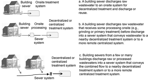

    

    Illustration of several scenarios with different wastewater conveyance options

  • • Basic features of collection and conveyance options include:

    • ○ Each building has internal drainage piping that collects wastewaters from fixtures and appliances

    • ○ Wastewater conveyed out of a building can be handled alone or combined with the wastewaters collected from other buildings

    • ○ Wastewater exits a building in a building sewer and can be fully treated and discharged or reused onsite, or be conveyed offsite to a nearby decentralized system, or be conveyed further away to a more centralized system

    • ○ Wastewater flows in sewers under gravity or pressure forces

• ■ Building drainage piping

  • • Fixtures and appliances are normally connected to drainage piping located within a building

  • • Building drainage piping systems are sized to handle intermittent discharges of fixture and appliance wastewaters

  • • Sizing is typically based on drainage fixture units (DFUs)

    • ○ 1 DFU is defined as a 7.5 gal/min discharge flow rate

  • • DFUs are assigned to each fixture or group of fixtures, e.g.:

    • ○ Toilet—1.6 gal gravity tank

      • * Private building = 3.0 DFUs

      • * Public building = 4.0 DFUs

    • ○ Clothes washer—automatic

      • * Private or public = 3.0 DFUs

  • • Pipe diameters and lengths depend on DFUs contributing

• ■ Drainage piping for buildings with source separation

  • • With source separation, modifications to conventional building drainage piping can be needed

    • ○ Two drainage networks are needed for:

      • * Urine diversion from a total wastewater stream

      • * Separating graywater and blackwater

    • ○ Three drainage networks are needed for:

      • * Separating graywater and blackwater plus urine diversion

  • • Installing modified drainage piping systems in buildings

    • ○ Easiest in new development or during major renovations

    • ○ In existing buildings, installation is possible, but more difficult to accomplish

• ■ Wastewater collection and conveyance in a sewer system

  • • A sewer system is comprised of pipelines, basins, pumps, controls, and other components that are used to collect and convey untreated or treated wastewaters from individual buildings to the site of treatment and discharge or reuse

  • • Conventional versus alternative sewer systems

    • ○ Conventional sewers—traditionally involves the collection and conveyance of raw or untreated wastewaters under gravity forces to a remotely located centralized treatment system for discharge or reuse

    • ○ Alternative sewers—typically involves collection and conveyance of processed or primary treated wastewaters under gravity or pressure forces to a decentralized treatment system for discharge or reuse or to a more remote centralized facility

• ■ Features of conventional gravity sewer systems

  • • Developed and used in the United States since the 1870s

  • • General design features include:

    • ○ Design capacity is based on the sewer flowing only half full (Fig. 5.2) for solids conveyance and cleaning equipment

      Fig. 5.2

      

      Cross-section of a typical gravity sewer

    • ○ Minimum diameter is usually >8-in. diameter

    • ○ Installed to provide a consistent slope with velocities > 2 ft/s

      • * Can lead to deep excavations and need for pumping stations to maintain slopes in areas with varied topography

    • ○ Access ports (manholes) for inspection and cleaning are provided at each change in slope or alignment, but usually no further apart than 400 ft.

    • ○ Installation of conventional gravity sewers can be very disruptive and costly as illustrated in Fig. 5.3

      Fig. 5.3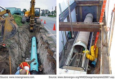

      

      Photographs of conventional sewer line installation5.8

• ■ Features of alternative sewer systems

  • • Alternatives were developed and used in the United States starting in the 1970s to reduce the high cost of conventional gravity sewers in rural and peri-urban areas

    • ○ The alternatives include two general features:

      • * Wastewater processing or treatment near buildings so wastewater solids are removed or reduced in size

      • * Use of small diameter pipes with watertight joints that are installed at shallow depths below the ground surface

    • ○ There are four alternatives that include:

      • * Septic tank effluent gravity sewers

      • * Septic tank effluent pressure sewers

      • * Raw wastewater grinder pump pressure sewers

      • * Raw wastewater vacuum sewers

    • ○ Features of these alternatives are highlighted in Table 5.1 and briefly described in the following pages

      Table 5.1 Representative features of alternative sewer systems

  • • Septic tank effluent gravity sewers

    • ○ Wastewater from a source is treated in a septic tank near the source and then septic tank effluent (STE) in collected and conveyed in a small diameter gravity sewer system

      • * These effluent sewers have several names, including:

        • – Septic tank effluent gravity sewers (STEG), small-bore sewers, effluent drains

        • – In the United States they are called STEG systems

    • ○ General design features include:

      • * Sewers can be designed to flow full or nearly full (Fig. 5.4) and small diameter pipes can be used (e.g., 2 in.)

        Fig. 5.4

        

        Cross-section of a STEG sewer

      • * Installation can be shallower and at variable slopes and

      • *  ≥2 ft/s scouring velocities are not needed

      • * Watertight joints and fewer access points can yield low I&I

  • • Septic tank effluent pressure sewers

    • ○ Wastewater from a source is treated in a septic tank near the source and then STE is pumped into a small diameter pressurized sewer system for collection and conveyance

      • * These effluent sewers are referred to as STEP systems

    • ○ General design features include:

      • * Sewers can be designed to flow full (Fig. 5.4) and small diameter pipes can be used (e.g., 1.5 in.) (Fig. 5.5)

        Fig. 5.5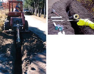

        

        Photographs illustrating the installation of a septic tank effluent pressure sewer (STEP) in a rural development area. Installation is made using a continuous trencher (left) and insulation can be added for shallow burial in cold climates (top). (Photographs courtesy of R.J. Otis)

      • * Installation can be shallower and at variable slopes and ≥ 2 ft/s scouring velocities are not needed

      • * Watertight joints and fewer access points can yield low I&I

      • * STEP systems can be favorable over STEG systems in hilly terrain where gravity is not capable of moving STE to a location targeted for treatment operations

  • • Grinder pump pressure sewer systems

    • ○ Wastewater flows by gravity from a building into a nearby sump containing a grinder pump (Fig. 5.6)

      Fig. 5.6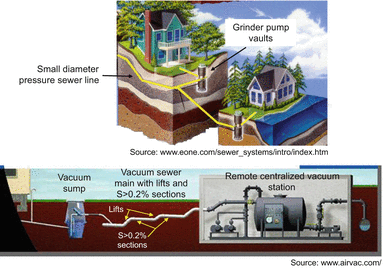

      

      Illustration of the key components of a grinder pump pressure sewer system (top) and a vacuum sewer system (bottom)

      • * The grinder pump is turned on periodically by float controls and it chops up the raw wastewater and reduces the heterogeneous mix of solids and objects into a slurry

      • * The pump discharges the wastewater slurry into a small diameter pressure sewer system

    • ○ General design features include:

      • * Sewers can be designed to flow full and small diameter pipes can be used (e.g., 2 in.)

      • * Installation can be shallower and at variable slopes but the velocity achieved in the pressure sewer has to achieve scouring and solids conveyance (e.g., ≥2 ft/s)

      • * Watertight joints and fewer access points can yield low I&I

  • • Vacuum sewer systems

    • ○ A vacuum pump in a remote collection station maintains a vacuum of 15–20 in. Hg on the main sewer lines (Fig. 5.6)

      • * Wastewater from a building flows to a sump separated from a vacuum sewer main by a vacuum valve

      • * When a volume of wastewater accumulates, a vacuum valve is opened and air and wastewater is sucked into the main sewer

      • * The wastewater flow is two phase (air and water), which can break down larger solids and aid conveyance

    • ○ General design features include:

      • * Sewers are designed to flow partially full at velocities that achieve scouring and solids conveyance (e.g., ≥ 2 ft/s)

      • * Small diameter pipes (e.g., 4 in.) are installed at shallow depths

      • * Watertight joints and fewer access points can limit I&I

• ■ Conditions that are well-suited for alternative sewers

  • • The existing or new development is located in an area with level or varied topography, shallow bedrock, or high ground water

  • • Wastewater needs to be collected from a cluster of buildings, a housing development, or town that has:

    • ○ Larger lot sizes (e.g., >0.5 acres) or limited connections per mile of sewer line (e.g., <100) (Fig. 5.7)

      Fig. 5.7

      

      Examples of a small town (left) and lower density rural housing development (right) where there are larger lot sizes and would be limited connections per mile of sewer line

    • ○ Existing or potential for onsite treatment or processing

5.1.1.2 5-2. Principles and Processes

• ■ Conveyance using small-bore sewers

  • • Small-bore sewer systems do not handle gross solids and debris or high concentrations of total suspended solids (TSS) and fats, oils and greases (FOG)

  • • In STEG and STEP systems, a septic tank (Chap. 6) is used for primary treatment at each building in a development to produce an effluent that is suitable for small-bore conveyance

  • • Small-bore sewers can also be used for other wastewaters

    • ○ Wastewater effluents with low solids contents that are produced by unit operations other than septic tanks (e.g., aerobic unit, porous media biofilter, etc.)

    • ○ Graywater (e.g., untreated or after a settling basin)

  • • Chapter 5 is focused on small-bore sewers for conveyance of septic tank effluent (STEG and STEP systems)

• ■ Alternative sewer system types and layouts

  • • The outlet is the terminus of the sewer system that collects wastewater effluent from the buildings within a development

  • • The outlet elevation relative to the elevation within a development guides suitability for each system (Fig. 5.8)

    Fig. 5.8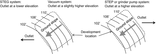

    

    Illustration of topographic conditions and the collection network outlet location as it relates to the suitability of using a particular alternative sewer system

  • • Development of effluent sewer system layouts

    • ○ Topographic base maps enable system layout and design

    • ○ Based on the outlet location, a system type is chosen

    • ○ Sewer line layouts can then be selected to suit the development

      • * Consider landscape features and try to minimize disruption to structures, roads, and other features

      • * Consider options for dividing the collection network into segments

        • – Segments are used to enable rational upsizing of sewer pipe diameters as more flow is accumulated toward the outlet

        • – A new segment is also typically used downstream of the junction of multiple segments

    • ○ Figures 5.9 and 5.10 illustrate a STEG and STEP system as laid out for the Mines Park development of 26 apartment buildings located on the Colorado School of Mines campus

      Fig. 5.9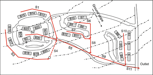

      

      Illustration of a STEG system serving a development of 26 apartment buildings (denoted by B1, B2, etc.). Note: The STEG system has 11 segments denoted as S1, S2, etc.

      Fig. 5.10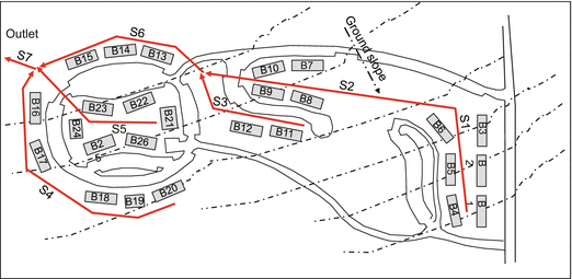

      

      Illustration of a STEP system serving a development of 26 apartment buildings (denoted by B1, B2, etc.). Note: The STEP system has 7 segments denoted as S1, S2, etc. Segment S1 and S2 could be combined into a single segment if the majority of the flow originates from the upstream end

  • • Cross sections are used to show elevation and length as illustrated in Fig. 5.11.

    Fig. 5.11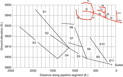

    

    Topographic cross-section of the 11 segments within a STEG system serving a development of 26 apartment buildings as shown in Fig. 5.9

• ■ Equivalent dwelling units (EDU)

  • • The EDU concept is used to normalize the discharges from different types of sources connected to a sewer

    • ○ For example, there can be houses, restaurants, schools, etc.

    • ○ An EDU is based on a selected average daily flow rate

      • * Designers or authorities can decide on the gal/d per EDU

      • * Based on Q_A for a DU, 150–250 gal/day per EDU is typical

  • • Calculating the number of EDUs

    • ○ For a single building or other source, Eq. 5.1 is used

      $$ \mathrm{E}\mathrm{D}\mathrm{U}=\frac{{\mathrm{Q}}_{\mathrm{A}}}{{\mathrm{Q}}_{\mathrm{EDU}}} $$

      (5.1)

      Where:

      • EDU = number of equivalent dwelling units (no.)

      • Q_A = average daily flow from a building or other source (gal/d)

      • Q_EDU = defined daily flow per EDU (gal/d per EDU) (e.g., 150–250 gal/day)

    • ○ For multiple buildings or other sources, Eq. 5.2 can be used

      $$ {\mathrm{N}}_{\mathrm{EDU}}={\displaystyle \sum_{\mathrm{B}=1}^{\mathrm{n}}\mathrm{B}=}\left(\frac{{\mathrm{Q}}_{\mathrm{A}1}+{\mathrm{Q}}_{\mathrm{A}2}+\cdots {\mathrm{Q}}_{\mathrm{A}\mathrm{n}}}{{\mathrm{Q}}_{\mathrm{EDU}}}\right) $$

      (5.2)

      Where:

      • N_EDU = number of equivalent dwelling units (no.)

      • B = building or other source

      • Q_A1…An = average daily flow from a building or other source (gal/d)

      • Q_EDU = defined daily flow per EDU (gal/d per EDU)(e.g., 150–250 gal/day)

    • ○ Example calculation results are shown in Table 5.2

      Table 5.2 Results of EDU calculations for several building and source conditions

  • • Determining the number of EDUs for sizing a particular segment within a sewer system

    • ○ EDUs for sizing a segment include the EDUs from any upstream segments plus those from buildings attached to the segment

    • ○ Equation (5.3) can be used to calculate the number of EDUs contributing to the segment being sized

      $$ {\mathrm{N}}_{\mathrm{EDU}}={\displaystyle \sum_{\mathrm{S}=1}^{\mathrm{n}}\mathrm{U}\mathrm{pstream}\kern0.5em \mathrm{E}\mathrm{D}\mathrm{U}}+{\displaystyle \sum_{\mathrm{B}=1}^{\mathrm{n}}\mathrm{Segment}\kern0.5em \mathrm{E}\mathrm{D}\mathrm{U}} $$

      (5.3)

      Where:

      • N_EDU = number of equivalent dwelling units contributing to a segment (no.)

      • Upstream EDU = EDUs contributing via an upstream segment (S_1…n)

      • Segment EDU = EDUs of buildings attached to the segment (B_1…n)

      • B_1…n = building or other source connected to the segment being sized

      • S_1…n = upstream segment(s) contributing to the segment being sized

    • ○ For the example segment shown in Fig. 5.12, N_EDU = 134 and this would be used to size the segment

      Fig. 5.12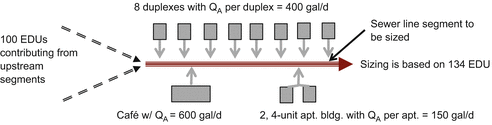

      

      Example calculation of the number of EDUs contributing to a sewer line segment where there are upstream EDUs contributing plus EDUs from buildings connected directly to the segment

      $$ {\mathrm{N}}_{\mathrm{EDU}}={\displaystyle \sum_{\mathrm{S}=1}^{\mathrm{n}}\mathrm{U}\mathrm{pstream}\kern0.5em \mathrm{E}\mathrm{D}\mathrm{U}}+{\displaystyle \sum_{\mathrm{B}=1}^{\mathrm{n}}\mathrm{Segment}\kern0.5em \mathrm{E}\mathrm{D}\mathrm{U}} $$

      (5.3)
      $$ {\mathrm{N}}_{\mathrm{EDU}}=100+\left[\left(\frac{8\times 400}{150}\right)+\left(\frac{600}{150}\right)+\left(\frac{2\times 4\times 150}{150}\right)\right]=133.3\Rightarrow 134 $$

  • • EDUs accumulate as you go from one segment to the next toward the outlet as illustrated in Fig. 5.13

    Fig. 5.13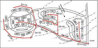

    

    Illustration of how EDUs accumulate in a STEG system serving a development of 26 apartment buildings as shown in Fig. 5.9. Note: There are 11 segments and the N_EDU shown are equal to the accumulated number at the end of each segment including the N_EDU from all upstream segments plus the N_EDU from buildings connected to the segment

    • ○ EDUs accumulating in an effluent sewer system is analogous to water flows increasing as you go downstream in a river system

• ■ Q_DP values for sizing a segment

  • • Q_DP = design flow rate (gal/min) for sizing a segment if it has a certain number of EDUs contributing to it

  • • Q_DP values can be affected by the type of sewer system, e.g.:

    • ○ STEG systems

      • * Effluent leaves a septic tank by gravity and enters the sewer

      • * Discharges from a septic tank are usually <1 gal/min, often in the 0.3–0.6 gal/min range, with periods of zero flow

    • ○ STEP systems

      • * Effluent is periodically pumped into the sewer

      • * In STEP systems, commonly used pumps discharge in the range of 5–20 gal/min

      • * Each connection has long periods of zero flow with periodic bursts of 5–20 gal/min flow

      • * Need to consider the particular pump’s discharge rate plus the probability of multiple pumps discharging simultaneously

    • ○ Q_DP values for sizing alternative sewer systems

      • * Data has been obtained by monitoring operating STEP systems serving residential developments and small towns (Fig. 5.14)

        Fig. 5.14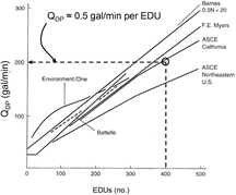

        

        Q_DP values versus cumulative EDUs. Source: Fig. 2.12 in USEPA 1991 shown as Fig. 6.3. Crites and Tchobanoglous 1998 Notes: • These Q_DP data are for STEP systems. • Data are based on monitoring of systems with older water-using fixtures and appliances contributing to the total wastewater flows. • It is uncertain how this might change for sources with modern water efficient plumbing or just graywater

  • • Estimating Q_DP for sizing a segment

    • ○ Q_DP might be estimated from monitoring data for existing systems

    • ○ It is more common to make predictions of Q_DP using Eq. 5.4

      $$ {\mathrm{Q}}_{\mathrm{DP}}=\kern0.5em {\mathrm{Q}}_{\mathrm{MIN}}+{\mathrm{Q}}_{\mathrm{EDU}}\left({\mathrm{N}}_{\mathrm{EDU}}\right) $$

      (5.4)

      Where:

      • Q_DP = design peak flow at a location in the sewer system (gal/min)

      • Q_MIN = minimum discharge rate from one EDU (gal/min)

      • = values of 10–20 gal/min are often used to account for the peak flow rate from one or a few buildings

      • Q_EDU = discharge per EDU for the development size (gal/min per EDU)

      • = values of 0.5 gal/min are typically used for systems with 50 or more connections

        Notes: The actual Q_MIN for a STEG system equals the likely peak rate of gravity discharge from a single septic tank that can be 1 gal/min or less depending on the building being served. The actual Q_MIN for a STEP or grinder pump system is often in the 10 to 25 gal/min range based on the type of pump used and its discharge rate. Also, flow controllers in a discharge line can maintain the pump discharge in the range of 10 gal/min. The actual Q_MIN from a vacuum vault can be 100 gal/min but this flow rate is rapidly attenuated in the vacuum sewer line.

      • N_EDU = number of EDUs contributing to Q_DP at a particular location

    • ○ Examples of Q_DP for sizing sewer line segments with varied numbers of EDUs contributing

    • ○ The Q_DP values shown in the Table 5.3 are calculated using Eq. 5.4

      Table 5.3 Examples of Q_DP values for sewer line segments with varied EDUs

• ■ Hydraulics of flow to handle the design peak flow

  • • Calculating velocity and head loss

    • ○ Velocity calculations can be made using the Hazen-Williams equation (Eq. 5.5) with substitutions for R (Eq. 5.6) and S (Eq. 5.7) for round pipes flowing full:

      

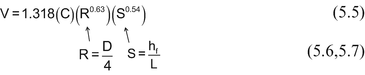
      Where:

      • V = velocity of flow (ft/s)

      • C = Hazen-Williams coefficient (−) (depends on pipe type and condition: C = 150 for new PVC pipe; C = 120–140 is used to account for aging)

      • R = hydraulic radius (flow area divided by wetted perimeter) (ft)

      • S = slope of energy grade line (ft/ft)

      • D = true inside pipe diameter (ft)

      • h_f = head loss due to friction (ft)

      • L = length of pipeline (ft)

    • ○ Head loss calculations

      • * To calculate head loss (h_f) due to flow in a pipeline segment, flow rate needs to be calculated (Eq. 5.8)

        $$ \begin{array}{l}{\mathsf{Q}}_{\mathsf{CAP}}=\left(\mathsf{V}\right)\times \left(\mathsf{A}\right)=\left[\left(\mathsf{1}.\mathsf{318}\mathsf{C}\right){\left(\frac{\mathsf{D}}{\mathsf{4}}\right)}^{\mathsf{0}.\mathsf{63}}{\left(\frac{{\mathsf{h}}_{\mathsf{f}}}{\mathsf{L}}\right)}^{\mathsf{0}.\mathsf{54}}\right]\times \left(\frac{\mathsf{\pi}{\mathsf{D}}^{\mathsf{2}}}{\mathsf{4}}\right)\end{array} $$

        (5.8)

        Where:

        • Q_CAP = flow rate capacity for a given pipe size and EGL slope (ft³/s)

        • V = flow velocity (ft/s)

        • A = pipe inside cross-sectional area (ft²)

        • D = true inside pipe diameter (ft)

        • h_f = head loss due to friction (ft)

        • L = length of pipeline (ft)

        • C = Hazen-Williams coefficient (−) (depends on pipe type and condition:

        • C = 150 for new PVC pipe; C = 120–140 is used to account for aging)

      • * Head loss (h_f) can be calculated by rearranging Eq. 5.8 to yield Eq. 5.9:

        $$ {\mathsf{h}}_{\mathsf{f}}=\mathsf{4}.\mathsf{72}\left(\mathsf{L}\right){\left(\frac{{\mathsf{Q}}_{\mathsf{C}\mathsf{AP}}}{\mathsf{C}}\right)}^{\mathsf{1}.\mathsf{85}}{\left(\mathsf{D}\right)}^{-\mathsf{4}.\mathsf{87}} $$

        (5.9)

        Equation (5.10) applies when the flow rate is in gal/min and the pipe diameter is in inches:

        $$ {\mathsf{h}}_{\mathsf{f}}=\mathsf{10}.\mathsf{5}\left(\mathsf{L}\right){\left(\frac{{\mathsf{Q}}_{\mathsf{C}\mathsf{AP}}}{\mathsf{C}}\right)}^{\mathsf{1.85}}{\left(\mathsf{D}\right)}^{-\mathsf{4.87}} $$

        (5.10)

        Where:

        • h_f = head loss (ft)

        • L = length of pipeline segment (ft)

        • Q_CAP = flow rate capacity for a given pipe size and EGL slope (gal/min)

        • C = Hazen-Williams coefficient (−) (depends on pipe type and condition: C = 150 for new PVC pipe; C = 120 to 140 is used to account for aging)

        • D = true inside pipe diameter (in.)

  • • Selection of a pipe type and diameter for a segment

    • ○ Tables and charts relate Q_CAP for pipe sizes to S and V

      • * For example, if sizing a STEP segment where Q_DP = 60 gal/min, new 3-in. diameter Class 200 pipe appears okay since S = 0.7 % and V = 2.45 ft/s (Table 5.4)

        Table 5.4 Q_DP values for different slope and velocity values to aid initial pipe size selection

    • ○ Calculations for pipe sizing need to account for pipe attributes

      • * Need to use true inside diameters which vary based on the nominal size and type of pipe (Table 5.5)

        Table 5.5 True inside diameters of pipes of different types and sizes

      • * Need to use roughness coefficients that reflect pipe aging

        • – For example use Hazen-Williams C values of 120 to 140 rather than 150, which applies to new plastic pipe

  • • Hydraulic and energy grade lines

    • ○ Hydraulic grade line (HGL)

      • * Represents the potential energy of a liquid in a pipeline

    • ○ Energy grade line (EGL)

      • * Represents potential plus kinetic energy along a pipeline

      • * Kinetic energy is determined by the velocity of flow (V)

      • * In most systems, V is low and contributes little to the EGL

        • – For example with V = 10 ft/s, the velocity head = 1.5 ft.

    • ○ For alternative sewers, the HGL ≈ EGL

      • * Velocity head can usually be ignored

      • * STEG systems—HGL is fixed based on ΔElevations

      • * STEP, grinder pump, vacuum systems—HGL depends on pump or vacuum discharge characteristics

    • ○ During flow in a pipe, friction causes head losses that reduce the head available for flow

    • ○ Head loss during flow at different rates in different pipe sizes is shown in Table 5.6

      Table 5.6 Headloss during flow in a full section of a sewer pipe

      • * For example: In a new 3-in. pipeline at S = 0.7 %, the Q_CAP = 60 gal/min and the headloss h_f = 7.0 ft per 1000 ft of length

  • • Development of the EGL

    • ○ An EGL can be developed for STEG, STEP and grinder systems but vacuum systems are more complicated due to the flow regime

    • ○ The EGL is based on calculated head losses (h_f) during flow in the segments of the STEG, STEP or grinder pump system

      • * For example, for a 3 segment system where segment 1 leads to the outlet:

        • – The h_f required to transport Q_DP in Segment 1 is added to the elevation of the static head, which equals the outlet elevation

        • – The h_f for Q_DP in Segment 2 is added to the elevation of the upstream end of Segment 1

        • – The h_f for Q_DP in Segment 3 is added to the elevation of the upstream end of Segment 2

        • – This process is used to establish the EGL pressure head in the main sewer line and in STEP or grinder pump systems, the total dynamic head (TDH) required for a pumping unit

    • ○ Examples of EGLs for a STEG system and STEP system are shown in Figs. 5.15 and 5.16

      Fig. 5.15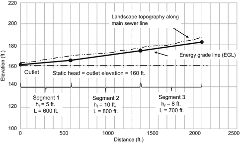

      

      Illustration of an EGL along 3 segments of a STEG system

      Fig. 5.16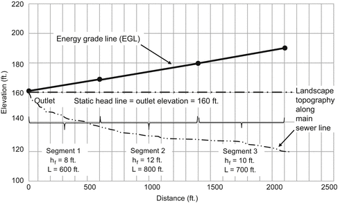

      

      Illustration of an EGL along 3 segments of a STEP system

  • • Pumps used in STEP or grinder pump systems

    • ○ Type of pump

      • * STEP systems and grinder pump systems utilize high-head, low-flow rate pumps

      • * This ensures the pumps can pressurize the sewer system at levels sufficient to transport the Q_DP in the main sewer lines and achieve needed velocities

      • * Often one type and size of pump can be used throughout a sewer system serving a development

    • ○ Pumps operate intermittently, based on float controls

      • * Pumps may cycle on 3 to 5 +/− times a day

      • * Discharge of 50 gal will draw down the water surface in a tank with 20 ft² of surface area by only 4 in.

    • ○ Pumps used in STEP systems are selected and set up to discharge at low rates (e.g., 5–20 gal/min)

      • * Low pumping rates out of the septic tanks help ensure limited turbulence in the tank and minimum solids carry over

    • ○ The TDH for a pumping unit is illustrated in Fig. 5.17 and calculations can be made using Eq. 5.11

      Fig. 5.17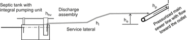

      

      Illustration of TDH components in a STEP system

      $$ \mathrm{T}\mathrm{D}\mathrm{H}={\mathrm{h}}_{\mathrm{p}}+\left({\mathrm{h}}_{\mathrm{e}}+{\mathrm{h}}_{\mathrm{h}\mathrm{v}}+{\mathrm{h}}_{\mathrm{l}}\right) $$

      (5.11)

      Where:

      • TDH = total dynamic head for a particular pumping unit (ft)

      • h_p = pressure head needed to transport Q_DP flow in the main sewer line at the point where the service lateral connects to it (ft)

      • h_e = change in elevation between the water level in the septic tank and the service lateral connection point at the main sewer line (ft)

      • h_hv = friction losses in the discharge assembly at a pumping unit (ft)

      • h_l = friction losses in the service lateral (ft) Note: h_hv + h_l are ~5 to 10 ft typ.

    • ○ The TDH that a pump could have to discharge against along 3 segments of a STEP system is illustrated in Fig. 5.18

      Fig. 5.18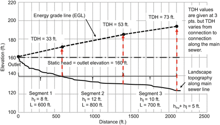

      

      Illustration of TDH along 3 segments within a STEP system

    • ○ A representative head-discharge curve for a high head pump used in a STEP system is shown in Fig. 5.19

      Fig. 5.19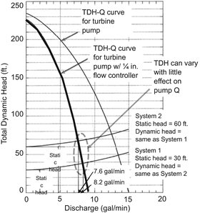

      

      Illustration of the head—discharge curve for a ½-hp high head submersible pump such as used in a STEP system. Note: Pumps are typically 0.5 to 1.5 hp. The pump discharge can be limited to 5 to 10 gal/min using a 1/4-in. flow controller in the discharge line. Also, a 1/8-in. bypass hole allows expulsion of trapped air and recirculation when the main sewer line pressure is too high. Source: From Orenco Systems^®, Inc. shown as Fig. 6.9 in Crites and Tchobanoglous 1998

5.1.1.3 5-3. Design and Implementation

• ■ Design and implementation (D&I) considerations for STEG and STEP systems

  • • Development features

  • • Typical design parameter values

  • • Type of pipe

  • • Approach to pipeline sizing

  • • Pipe size suitability

  • • System components

  • • Hybrid systems

  • • Special considerations

  • • System installation

  • • System O&M

    Note: This section is focused on STEG and STEP systems since they are most widely used in decentralized infrastructure applications. Elements of the design process used for STEP systems also applies to grinder pump systems but vacuum sewer systems are more complicated. Design and implementation of STEP, grinder pump, and vacuum sewer systems is often completed with the involvement of one of the major technology vendors and equipment manufacturers (e.g., Orenco Systems®, Inc., Environment One, AIRVAC®, respectively).

• ■ D&I considerations —Development features

  • • Land use and development attributes

    • ○ Type and number of buildings and wastewater sources

    • ○ Density of the development

    • ○ Planned development growth in the future, if any

    • ○ Location of the site for treatment and discharge or reuse

  • • Topography

    • ○ Level or gently sloping vs. hilly and mountainous terrain

  • • Subsurface characteristics

    • ○ Depth of soil and presence of shallow bedrock

    • ○ Depth to ground water

    • ○ Depth of freezing zone (if applicable)

• ■ D&I considerations—Typical design parameters

  • • Listed in Table 5.7 are the range of values that can be used for different design parameters for STEG and STEP systems

    Table 5.7 Representative values for different design parameters for STEG and STEP systems

• ■ D&I considerations —Type of pipe

  • • Different types of plastic pipe can be used in STEG and STEP systems (Table 5.8)

    Table 5.8 Features of different types of plastic pipe used for STEG and STEP systems

    Table 5.9 Q_DP values for different slope and velocity values to aid initial pipe size selection

• ■ D&I considerations—Approach to pipeline sizing

  • • STEG systems

    • ○ EGL slope is determined by gravity given the site topography

    • ○ Pipe diameters have to be large enough so that under a given S the sewer line Q_CAP exceeds the Q_DP

    • ○ Typically the Q_DP will be only a fraction of the capacity available (Q_CAP), so at times the pipe may not flow full

  • • STEP systems

    • ○ EGL slope is determined by the pumping units selected to transport the Q_DP and the TDH during system operation

    • ○ Typically, the Q_CAP will be equal to the design peak flow rate the system is designed for (i.e., Q_DP) and the pipe will flow full

  • • Steps followed during sizing a segment in a STEG system

    • ○ Determine the N_EDU contributing and calculate the Q_DP

    • ○ Determine the length of the sewer line segment

    • ○ Determine the drop in elevation and slope

    • ○ Select a trial pipe diameter to handle Q_DP at S and suitable V

    • ○ Calculate the velocity assuming the pipe is flowing full (check that V is near or < 5 ft/s)

    • ○ Calculate the pipe cross-sectional area

    • ○ Calculate the pipe capacity (Q_CAP) when flowing full

    • ○ Compare Q_DP to the flowing full capacity, Q_CAP

      • * Q_DP/Q_CAP < 1: pipeline segment flows only partially full

      • * Q_DP/Q_CAP > 1: surcharge flow occurs during peak Q

      • * Q_DP/Q_CAP >> 1: repeat calculations with a larger pipe diameter

  • • Steps followed during sizing a segment in a STEP system

    • ○ Determine the N_EDU contributing and calculate Q_DP

      • * Note that the required Q_CAP = Q_DP

    • ○ Determine the length of the sewer line segment

    • ○ Select a trial pipe diameter to handle Q_DP at suitable S and V

    • ○ Calculate the slope of the energy grade line (EGL) for the pipe segment (confirm that S is reasonable, e.g., 0.5–1.5 %)

    • ○ Calculate the pipe cross-sectional area

    • ○ Determine the velocity by dividing the Q_CAP by the cross-sectional area (confirm that V is reasonable, near or < 5 ft/s)

    • ○ Calculate the head loss due to friction (h_f) based on S and L

    • ○ Plot the EGL on the system profile to determine the TDH each pump would have to discharge against

• ■ D&I considerations —Pipe size (diameter) suitability

  • • Suitability based on EGL slope

    • ○ For many systems, designs can yield an EGL S = 0.5–1.5 %

      • * Minimum slopes

        • – The system EGL S to the outlet must be > 0.0 %

        • – If S for a segment is too low, it could indicate the pipe size is bigger than needed

      • * Maximum slopes

        • – For some STEG systems, S can be high (e.g., >1.5 %)

        • – If S is too high in STEP systems, it indicates the pipe diameter is too small and energy due to pumping is being wasted

    • ○ S can be controlled by topography

      • * For a STEG system, S is largely controlled by landscape topography and it can be >1.5 %

      • * For a STEP system, topography will not control S since pumps can be selected to yield a desired S

  • • Suitability based on flow velocity (V)

    • ○ For many systems, designs can yield V < 5 ft/s

      • * Minimum velocities

        • – Technically a minimum V is not required

        • – But some regulatory agencies can require one

          •       e.g., V minimum = 1.0–1.5 ft/s during peak Q

      • * Maximum velocities

        • – To avoid excessive friction losses and damage to fittings and valves, particularly in STEP systems, try to keep V < 5 ft/s

    • ○ V can be affected by topography

      • * For STEG systems, V can be controlled in part by landscape topography which controls S

      • * For STEP systems, topography won’t control V since pumps can be selected to yield a desired S and V

• ■ D&I considerations—System components

  • • STEG system components

    • ○ Onsite components

      • * Septic tank (potentially including an effluent screen)^a

        ^aSeptic tank units are described in Chap. 6. One septic tank can serve multiple buildings. If septic tanks are already existing but are old, they may need to be replaced with watertight, properly sized and installed units.

      • * Service laterals from each septic tank to the sewer main

    • ○ Collection system components

      • * Check valves and shutoff valves on the service lateral

      • * Small diameter gravity flow sewer line segments

      • * Cleanouts at certain locations

      • * Vents and and combinations of air release/vacuum valves

      • * Corrosion and odor control options

    • ○ An illustration of STEG onsite system components in Fig. 5.20

      Fig. 5.20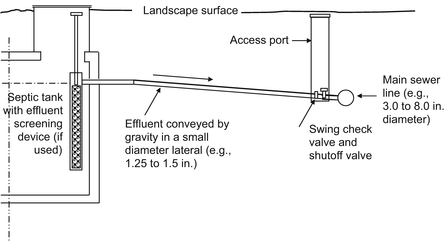

      

      Illustration of the onsite system components of a STEG system

  • • STEP system components

    • ○ Onsite components

      • * Septic tank with effluent screen^b

        ^b Notes: One septic tank can serve multiple buildings. If septic tanks are already existing but are old, they may need to be replaced with watertight, properly sized and installed units.

      • * Pumping unit with pressurized lateral to a sewer main

    • ○ Collection system components

      • * Check valves and shutoff valves on the service lateral

      • * Small diameter pressurized sewer lines

      • * Cleanouts at certain locations

      • * Valves placed throughout the system

        • – Air release valves

        • – Pressure sustaining valves

      • * Corrosion and odor control options

    • ○ Illustrations of STEP onsite system components are shown in Figs. 5.21 and 5.22

      Fig. 5.21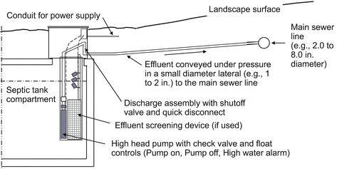

      

      Illustration of the onsite system components of a STEP system (Orenco Systems^®, Inc.)

      Fig. 5.22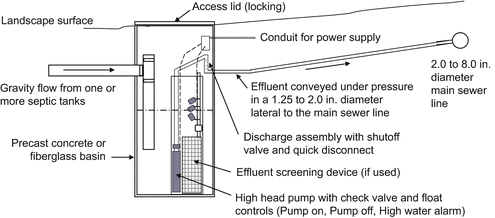

      

      Illustration of an external pumping unit for a STEP system

  • • Collection system components

    • ○ Air release valves (Fig. 5.23)

      Fig. 5.23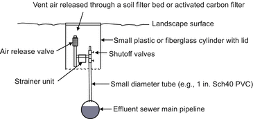

      

      Illustration of an air release valve setup

      • * Used at high points to release air that can accumulate

    • ○ Pressure sustaining valves

      • * Used to maintain upstream static pressures in those portions of a STEP system which are higher in elevation than the outlet

    • ○ Cleanouts

      • * In STEG or STEP systems cleanouts can facilitate cleaning of one or more pipeline segments if needed (Fig. 5.24)

        Fig. 5.24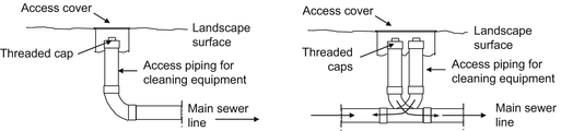

        

        Illustration of cleanouts used in STEG systems at the end of a terminal segment (left) and along a segment (right)

      • * However, cleaning has rarely been required even in systems that have been operating for decades

      • * Cleanouts are typically installed at just a few locations, e.g.:

        • – Ends of terminal pipe segments

        • – Pipe junctions or pipe size changes

• ■ D&I considerations—Hybrid systems

  • • Developments can be served by individual STEG or STEP systems or hybrids

  • • Examples of hybrid systems include:

    • ○ A STEG system used for most of a subdivision development with a STEP system used for part of it (based on area-wide topography), the combination of which are conveyed to the treatment site

    • ○ A STEG or STEP system, which discharges into a conventional sewer system with gravity collection and conveyance of STE and raw wastewater to the treatment site

    • ○ A STEG system with a pump station at the outlet and pressurized force main that conveys STE to the treatment site

• ■ D&I considerations—Special considerations

  • • Air binding and air release valves

    • ○ Air can become entrapped in STEG or STEP sewers based on the variable grades that are used

    • ○ Air release valves are important to mitigate the air entrapment and its effects on flow capacity

    • ○ Air release valves are typically needed at high points of sewer lines where air can accumulate

    • ○ Air release valves can be manual or automatic

    • ○ The air released through an air release valve is typically treated in a soil bed or activated carbon filter before release to the atmosphere

    • ○ Air release valves are typically inspected on an annual basis

  • • Corrosion and odor

    • ○ STE that is conveyed in STEG or STEP sewers is low in dissolved oxygen and can contained reduced compounds such as H₂S

    • ○ When STE contacts air—such as during flow through a manhole and connection to a conventional gravity sewer or discharge into a treatment unit—there is potential for both corrosion and odor (sulfur compounds are often involved)

    • ○ Corrosion control options include:

      • * Limit exposure to air

      • * Provide corrosion resistance equipment such as plastic, stainless steel, or coated products

        • – Corrosion protection is especially important for electrical wiring

    • ○ Odor control devices can also be used

• ■ D&I considerations —Installation

  • • Installation practices are illustrated in Figs. 5.25, 5.26 and 5.27

    Fig. 5.25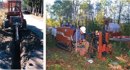

    

    Photographs of effluent sewer main installation using a continuous trencher (left) and directional drilling (right) methods. (Photographs courtesy of R. J. Otis)

    Fig. 5.26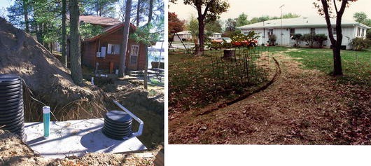

    

    Photographs of a septic tank/pump vault installation along a lakeshore development (left) and a service lateral run from a residence to the main sewer line (right). (Photographs courtesy of R. J. Otis)

    Fig. 5.27

    

    Photograph of insulated pipe used for shallow burial of sewer pipe in a cold climate. (Photograph courtesy of R. J. Otis)

• ■ D&I consideration—Operation and maintenance

  • • For STEG and STEP systems

    • ○ Septic tank operation and maintenance (refer to Chap. 6)

      • * Inspect tanks and measure solids accumulation at 1–3 years to estimate a solids removal frequency

        • – Solids that are removed periodically need to be properly managed

      • * Screening devices (if used) need to be cleaned annually

    • ○ Cleaning of a segment of the sewer system could be required to remove accumulating solids, though this is rarely needed

  • • For STEP systems (in addition to the above)

    • ○ The pumping equipment needs attention if an alarm condition occurs due to loss of power, blockage or other cause

    • ○ Pump replacement is needed at a frequency based on the pump design life (e.g., 20 years)

5.1.1.4 5-4. Summary

• ■ Decentralized infrastructure can require collection and conveyance of wastewaters

  • • Alternative sewer systems convey septic tank effluent from one or multiple sources under gravity (STEG) or pressure (STEP) or convey raw wastewater using grinder pumps and pressurized sewers or without grinding in vacuum sewers

• ■ STEG or STEP systems are widely used and offer potential benefits

  • • Use passive primary treatment of raw wastewater at a source

  • • Convey STE in small-diameter pipe with watertight joints laid at variable grades in shallow trenches without manholes

  • • Enable clustering of multiple sources and more efficient treatment and discharge or reuse based on economies of scale

5.1.1.5 5-5. Example Problems

• ■ 5EP-1. Design of a STEG system for Mines Park

  • • Given information

    • ○ A housing development is located on the Colorado School of Mines campus in Golden, Colorado

      • * The development characteristics are revealed in an aerial photograph (Fig. 5EP.1) and a topographic base map

        Fig. 5EP.1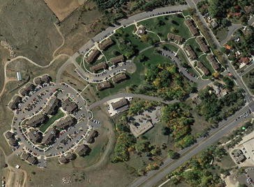

        

        Aerial photograph of the Mines Park housing development located on the campus of the Colorado School of Mines in Golden, Colorado USA

        • – There are 26 buildings with different numbers of apartments and occupants (Table 5EP.1)

          Table 5EP.1 Building information for the Mines Park development

      • * The effluent collected from the buildings will be discharged at the outlet shown to a membrane bioreactor with disinfection for nonpotable reuse within the development

    • ○ One EDU is defined as Q_A = 150 gal/day

  • • Determine

    • ○ Layout a STEG collection system for the development and complete the sizing calculations for Segment 1 of the system

  • • Solution

    • ○ Assumptions made:

      • * Building information is shown in Table 5EP.1

      • * Assume Q_A per DU = 80 % of 69.2 + 37.2N_P/DU (Eq. 3.2) where 80 % is used here since there are no clothes washers in the DUs

      • * Use Q_DP = 15 + 0.5N_EDU for all STEG segments

      • * Use Schedule 40 PVC pipe with C = 130 to account for aging; minimum pipe size = 2 in. (true ID = 2.067 in.)

    • ○ Layout a STEG collection system divided into segments

      • * One proposed layout is shown in Fig. 5EP.2

        Fig. 5EP.2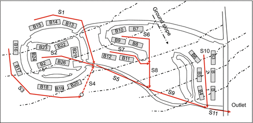

        

        STEG collection system layout for the Mines Park development. (Note: there are other layouts that could also work.)

    • ○ Contributing EDUs and design peak flows for each segment

      • * Determine the N_EDU contributing based on building information and layout (Table 5EP.1)

        • – N_EDU = upstream EDUs plus segment buildings EDUs

      • * Determine the design peak flows using Eq. 5.4 with Q_MIN = 15 gal/min and Q_EDU = 0.5 gal/min (Table 5EP.2)

        Table 5EP.2 EDUs contributing to each STEG segment in the Mines Park development

        $$ {\mathsf{Q}}_{\mathsf{DP}}=\kern0.5em 15+0.5\left({N}_{EDU}\right) $$

        (5.4)

    • ○ Complete the pipeline sizing calculations for Segment 1

      • * Segment 1 is highlighted in Fig. 5EP.3

        Fig. 5EP.3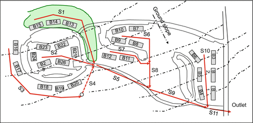

        

        STEG system layout for the Mines Park development with Segment 1 highlighted. (Note: there are other layouts that could also work.)

      • * Select a trial pipe diameter for Segment 1

        • – Use the calculated Q_DP for Segment 1 (Table 5EP.2)

        • – Using a topographic base map:

          • Determine the length of Segment 1

          • Determine the elevation drop over the pipe length

        • – Calculate the slope available

        • – Select a pipe diameter that appears able to handle Q_DP (for example using Table 5.4)

      • * Calculate the velocity of flow in Segment 1

        • – Use the slope and trial pipe diameter shown in Table 5EP.3 and the Hazen-Williams equation (Eq. 5.5)

          Table 5EP.3 Design peak flow and slope applicable for Segment 1 leading to a trial pipe diameter

        $$ \begin{array}{l}V=1.318(C)\left({R}^{0.63}\right)\left({S}^{0.54}\right)\\ {}V=1.318(130)\left[{\left(\frac{2.067/12}{4}\right)}^{0.63}\right]{(0.046)}^{0.54}\\ {}V=1.318(130)(0.138)(0.1896)\\ {}V=4.48\kern0.5em \mathrm{ft}/\mathrm{s}\end{array} $$

        (5.5)

      • * Calculate the segment capacity, Q_CAP, and compare it to the design flow rate, Q_DP (Table 5EP.4)

        Table 5EP.4 Segment 1 flow rate capacity compared to the design peak flow contributing to it

        $$ \begin{array}{l}{\mathrm{Q}}_{\mathrm{CAP}}=\mathrm{V}\times \mathrm{A}\\ {}{\mathrm{Q}}_{\mathrm{CAP}}=\left(4.48\kern0.5em \mathrm{f}\mathrm{t}./\mathrm{s}\right)\left(\frac{3.63\kern0.5em {\mathrm{in}}^2}{144 in./{\mathrm{ft}}^2}\right)\\ {}{\mathrm{Q}}_{\mathrm{CAP}}=0.113\kern0.5em \mathrm{f}{t}^3/\;\mathrm{s}\\ {}{\mathrm{Q}}_{\mathrm{CAP}}=0.113\kern0.5em {\mathrm{ft}}^3/\;\mathrm{s}\left(\frac{449\kern0.5em \mathrm{gal}/ \min }{1\kern0.5em {\mathrm{ft}}^3/\mathrm{s}}\right)=50.7\kern0.5em \mathrm{gal}/ \min \end{array} $$

        (5.8)

      • * Assessing suitability of pipeline sizing

        • – A 2-in. diameter pipe was selected for Segment 1 since:

          •   It appears to have the capacity to handle the Q_DP in the normal range of S (0.5–1.5 %) and V (<5 ft/s)

          •   2-in. diameter pipe is a minimum size often used for STEG mains

        • – The slope determined for the Segment 1 was higher than the normal 0.5–1.5 % due to topography at the site

        • – Due to the high slope and 2-in diameter size, the pipeline segment V is high (5.2 ft/s)

      • * Suitability?

        • – Reducing the diameter (say to 1.5 in.) would reduce V and A and reduce Q_CAP and thereby increase the utilization of the pipeline capacity (i.e., increase the ratio of Q_DP to Q_CAP from 0.48 toward 1.0)

        • – But, given the 2-in. diameter minimum sizing, pipeline sizing for Segment 1 is okay (even though it is somewhat oversized)

• ■ 5EP-2. Design of a STEP system for Mines Park

  • • Given information

    • ○ A housing development is located on the Colorado School of Mines campus

      • * The development characteristics are revealed in an aerial photo (Fig. 5EP.1) and a topographic base map

      • * There are 26 buildings with different numbers of apartments and occupants (Table 5EP.1)

      • * The effluent collected from the buildings will be discharged at the outlet to a soil-based treatment system located in the open space

    • ○ One EDU is defined as Q_A = 150 gal/day

  • • Determine

    • ○ Layout a STEP collection system for the development and complete the sizing calculations for Segment 1 of the system

  • • Solution^c

    ^cAssumptions made are the same as for Problem 5EP-1 except class 200 pipe is used

    • ○ Layout a STEP collection system divided into segments (Fig. 5EP.4)

      Fig. 5EP.4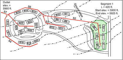

      

      STEP collection system layout for the Mines Park development with Segment 1 highlighted. (Note: there are other layouts that could also work.)

    • ○ Determine the design peak flows for each pipeline segment

      • * For a STEP system, determine Q_DP using Eq. 5.4 with Q_MIN = 15 gal/min and Q_EDU = 0.5 gal/min (Table 5EP.5)

        Table 5EP.5 Design peak flows for each segment of the STEP system in the Mines Park development

        $$ {\mathsf{Q}}_{\mathsf{DP}}=15+0.5\left({\mathrm{N}}_{\mathrm{EDU}}\right) $$

        (5.4)

    • ○ Select a trial pipe diameter for Segment 1

      • * Select a trial pipeline diameter to handle Q_DP = 28.5 gal/min

      • * Using Table 5.4, select a trial pipe size

        • – New 2-in. Class 200 pipe appears to have capacity to handle Q_DP at a suitable slope (0.5–1.5 %) and velocity (<5 ft/s)

    • ○ Calculate the slope (S) of the energy grade line (EGL) needed to convey the Q_DP in Segment 1 using Eqs. 5.7 and 5.10

      $$ \begin{array}{c}\hfill \begin{array}{l}S=\frac{h_f}{L}=10.5{\left(\frac{Q_{CAP}}{C}\right)}^{1.85}{(D)}^{-4.87}\\ {}S=10.5{\left(\frac{28.5\kern0.5em \mathrm{gal}/ \min }{130}\right)}^{1.85}{(2.149)}^{-4.87}\\ {}S=10.5(0.0603)(0.0241)\\ {}S=0.0153\kern0.5em \mathrm{ft}./\mathrm{ft}.=1.5\%\end{array}\hfill \end{array} $$

      (5.7, 5.10)

    • ○ Determine the velocity of flow in Segment 1

      • * Calculate the pipe cross-sectional area

      • * Divide the Q_DP (which = Q_CAP) by the cross-sectional area and determine V

        $$ \mathrm{A}=\frac{{\uppi \mathrm{d}}^2}{4}=\frac{3.1414{\left(\frac{2.149\kern0.5em \mathrm{in}.}{12\kern0.5em \mathrm{in}./\mathrm{ft}.}\right)}^2}{4}=0.0252\kern0.5em {\mathrm{ft}}^2 $$
        $$ \mathrm{V}=\frac{{\mathrm{Q}}_{\mathrm{CAP}}}{\mathrm{A}}=\frac{28.5\kern0.5em \mathrm{gal}/ \min }{\left(\frac{449\kern0.5em \mathrm{gal}/ \min }{{\mathrm{ft}}^3/\mathrm{s}}\right)}\left(\frac{1}{0.0252\kern0.5em \mathrm{f}{\mathrm{t}}^2}\right)=2.52\kern0.5em \mathrm{f}\mathrm{t}/\mathrm{s} $$

    • ○ Assessing the suitability of Segment 1 pipeline sizing

      • * A 2-in. diameter pipe was selected for Segment 1 since:

        • – It appeared to have the capacity to handle the Q_DP in the normal range of S (0.5–1.5 %) and V (<5 ft/s)

        • – 2-in. diameter is a size often used for STEP mains

    • ○ Suitability?

      • * The slope determined for Segment 1 was 1.5 %, which is okay since it is in the normal range of 0.5–1.5 %

      • * The velocity determined for Segment 1 was 2.5 ft/s, which is fine since it is less than the recommended 5 ft/s

    • ○ Calculate the head loss due to friction (h_f) based on S and L using Eq. 5.7

      $$ \begin{array}{l}{\mathrm{h}}_{\mathrm{f}}=\mathrm{S}\times \mathrm{L}\\ {}{\mathrm{h}}_{\mathrm{f}}=\left(0.015\kern0.5em \mathrm{ft}/\mathrm{ft}\right)\left(420\kern0.5em \mathrm{ft}.\right)=6.3\kern0.5em \mathrm{ft}.\end{array} $$

      (5.7)

    • ○ TDH components for Segment 1

      $$ \mathrm{T}\mathrm{D}\mathrm{H}={\mathrm{h}}_{\mathrm{p}}+\left({\mathrm{h}}_{\mathrm{e}}+{\mathrm{h}}_{\mathrm{h}\mathrm{v}}+{\mathrm{h}}_{\mathrm{l}}\right) $$

      (5.11)

      • * h_p = pressure head loss

        •  = 6.3 ft plus the sum of h_f for Segments 2–11

      • * h_e = elevation head loss

        • = outlet elevation—segment elevation

        •  = 5960 ft—5900 ft = 60 ft.

      • * h_hv = discharge assembly losses

      • * h_l = lateral headloss due to friction

        Typ. 5–10 ft.

References

References cited in Chap. 5 are listed along with other references that have content relevant to the topics covered in Chap. 5.
AIRVAC® (2015) AIRVAC vacuum sewers. Bilfinger AIRVAC Water Technologies, 200 Tower Drive, Unit A, Oldsmar, FL. http://www.airvac.com
Crites RW, Tchobanoglous G (1998) Small and decentralized wastewater management systems. McGraw-Hill, 1084 pp
Environment One (2015) E/One sewer systems. Environment One Corporation, 2773 Balltown Road, Niskayuna, NY. http://www.eone.com
Orenco Systems® (2012) Effluent sewer design manual. 56 pp. www.orenco.com
USEPA (1991) Manual for Alternative Wastewater Collection Systems. U.S. Environmental Protection Agency, EPA/625/1-91/024. October. 220 pp
Author information
Authors and Affiliations