Treatment Using Constructed Wetlands

Abstract

A constructed wetland is an engineered natural plant and water system that is designed to treat wastewater by exploiting the processes that occur within natural wetland ecosystems. This chapter describes the principles and processes that occur in constructed wetlands that are important to wastewater treatment and water reclamation. This chapter discusses the considerations important to design and implementation of free water surface and subsurface vegetated bed wetlands for use in decentralized systems.

Slides of Chapter 10 Decentralized Water Reclamation

10.1.1 Chapter 10: Treatment Using Constructed Wetlands

Contents

• 10-1. Introduction

• 10-2. Treatment performance

• 10-3. Principles and processes

• 10-4. Design and implementation

• 10-5. Summary

• 10-6. Example problems

10.1.1.1 10-1. Introduction

• ■ Constructed wetlands as a treatment unit operation

  • • Constructed wetlands used as a treatment unit operation in decentralized systems are designed to exploit the water renovation characteristics of natural wetland ecosystems

  • • Impaired water, wastewater, or sludge can be delivered as the influent to a constructed treatment wetland

    • ○ Influent delivery to the wetland can be passively done using gravity or via intermittent pumping

    • ○ Influent is distributed into the inlet of the wetland and flows through it to an outlet end

  • • Treatment occurs during long hydraulic retention times (e.g., days) primarily due to biological treatment and plant-based processes

  • • A constructed treatment wetland can also provide wildlife habitat and other aesthetic benefits

  • • Constructed treatment wetlands are among a variety of constructed land-based plant and water systems (Fig. 10.1)

    Fig. 10.1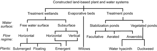

    

    Classification of constructed treatment wetlands within the constructed land-based plant and water systems

    • ○ Constructed treatment wetlands can be classified by water surface position, flow direction, and type of vegetation

  • • There are three major types of constructed treatment wetlands

    • ○ Horizontal flow free water surface wetlands (FWS)

      • * Used for stormwaters , acid mine drainage, oil and gas co-produced waters, wastewaters

      • * For wastewater applications, FWS wetlands are typically used for tertiary polishing of secondary effluents discharged from wastewater treatment plants

    • ○ Horizontal flow subsurface vegetated bed wetlands (VSB)

      • * Used for small flows wastewater applications, VSBs typically receive primary effluent as the influent and produce a secondary effluent

    • ○ Vertical flow subsurface vegetated bed wetlands (VVSB)

      • * Used for treatment of high strength wastewaters and sludge drying and treatment

  • • The features of the three types of wetlands are summarized in Table 10.1 and highlighted in the following pages

    Table 10.1 Summary of the key features of the major types of constructed treatment wetlands

  • • Features of a typical FWS wetland are shown in Fig. 10.2

    Fig. 10.2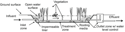

    

    Features of a typical horizontal flow free water surface constructed wetland

    • ○ Water surface is visible over most of the wetland, with open water zones and densely planted zones

    • ○ Wastewater enters the wetland and flow is horizontal from an inlet zone to an outlet zone, primarily through an open water zone that benefits treatment by aeration, volatilization, and photodegradation processes

    • ○ Vegetation can be emergent, floating, and/or submerged

  • • Features of a typical VSB wetland are shown in Fig. 10.3

    Fig. 10.3

    

    Features of a typical horizontal flow subsurface bed constructed wetland

    • ○ Water surface is below the top of the VSB and is not visible

      • * You can walk across a subsurface flow wetland

    • ○ Wastewater enters the inlet of the wetland and flow is horizontal through a saturated bed of planted porous media

    • ○ Vegetation is dominantly emergent vegetation

  • • Features of a typical VVSB wetland are shown in Fig. 10.4

    Fig. 10.4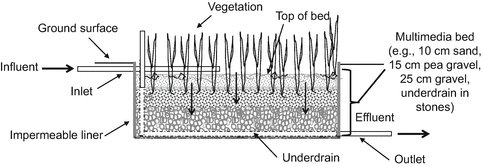

    

    Features of a typical vertical flow subsurface bed constructed wetland

    • ○ A VVSB wetland is a single pass, multimedia filter with vegetation

    • ○ Intermittent dosing of wastewater (or sludge) over the filter surface

    • ○ Flow is intermittent and vertical from the surface to an underdrain by downflow or upflow saturation, with holding and then drainage

• ■ Where are constructed treatment wetlands used?

  • • Where there is adequate land area available and a desire to utilize passive, natural treatment systems

  • • FWS wetlands have been used for tertiary polishing of secondary effluents to enable surface discharge and reuse of effluent (the wetland effluent may have to be disinfected first)

  • • VSB wetlands have been used to produce a secondary effluent often for discharge to a decentralized land-based treatment unit

  • • VVSB wetlands have been used for sludge dewatering

• ■ This chapter covers FWS and VSB constructed wetlands as used for treatment of wastewaters and other impaired waters

Note: From hereon in Chap. 10, constructed treatment wetlands will be referred to simply as constructed wetlands

10.1.1.2 10-2. Treatment Performance

• ■ Constructed wetlands are normally designed to achieve secondary treatment of primary effluents or tertiary polishing of secondary effluents

  • • BOD and TSS removal

    • ○ Typically occurs through biological processes (BOD) and sedimentation and filtration (TSS)

  • • N and P removal (depends on design and environment)

    • ○ N removal can occur via biological processes and also plant uptake and volatilization

    • ○ Phosphorus removal can occur by plant uptake^a and sorption

  • • Other pollutants and pathogens

    • ○ Removal (to some extent) is possible by various processes

    • ○ The open water surface in a FWS wetland enables volatilization and photodegradation processes

      ^a Note: removal by plant uptake is often only considered true removal if the plants are harvested and removed.

• ■ Treatment efficiency

  • • Removal efficiency (R_E) as illustrated in Fig. 10.5 can be calculated for a VSB or FWS using Eq. 10.1

    Fig. 10.5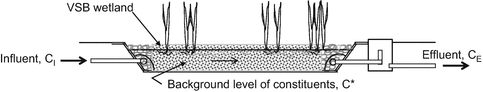

    

    Illustration of treatment efficiency achieved in a VSB constructed wetland

    • Treatment efficiencies for constituents of potential concern within a FWS or VSB wetland are presented in Table 10.2

    Table 10.2 Representative treatment efficiency achieved within a well designed and operated constructed wetland^a

    • $$ {\mathrm{R}}_{\mathrm{E}}=\left(\frac{\left({\mathrm{C}}_{\mathrm{I}}+\mathrm{C}*\right)-{\mathrm{C}}_{\mathrm{E}}}{{\mathrm{C}}_{\mathrm{I}}+\mathrm{C}*}\right)\times 100\% $$

      (10.1)

      Where:

      R_E = removal efficiency for C_I (%)

      C_I = influent concentration (mg/L)

      C* = background constituents (mg/L)

      C_E = effluent concentration (mg/L)

• ■ Constructed wetland effluent composition

  • • Factors affecting treatment efficiency and effluent composition

    • ○ Wetland type, surface area and volume provided to handle the design flow rate and remove constituents of concern

    • ○ Establishing and maintaining a plug-flow like regime through the wetland and avoiding short-circuiting and inactive flow zones

    • ○ Suitable local hydrologic and climatic conditions which are properly accounted for in system design and operation

  • • Modifications for enhanced treatment purposes

    • ○ Effluent recirculation instead of single pass flow

      • * Ability to recirculate partially or fully treated effluent may offer some modest improvements to performance, particularly in VSB wetlands

      • * Recirculation may add dissolve oxygen (DO) and reduce BOD and TSS concentrations in the wetland effluent

    • ○ Active aeration instead of passive aeration

      • * Aeration can be used to increase DO levels

        • – Using compressed air delivery to increase DO levels and improve removal of BOD

        • – Can create aerobic and anoxic zones and increase removal of nitrogen

    • ○ Use of reactive media in place of gravel in a VSB

      • * Media with surface reactivity can be used

        • – e.g., aggregates with high sorption for phosphorus

    • ○ Hybrid wetland systems

      • * Hybrid wetland systems can improve overall performance

      • * For example to polish BOD removal and enable improved denitrification, hybrids could include:

        • – Use of a VSB followed by VVSB

        • – Use of a FWS followed by a VSB

10.1.1.3 10-3. Principles and Processes

• ■ Natural wetlands in the environment

  • • Natural wetlands are located in land areas with hydric soils that are wet during part or all of the year

    • ○ Historically, wetlands have been referred to as:

      • * Swamps, Marshes, Bogs, Fens, Sloughs

    • ○ All wetlands are ‘wet’ long enough each year that they exclude plant and vegetation species that cannot grow in saturated settings

  • • Natural wetlands are complex ecosystems wherein a range of processes can occur, including:

    • ○ Hydrologic and hydraulic processes

    • ○ Purification processes: plant, microbial, physical, chemical

  • • Natural wetlands have the potential to transform common pollutants to harmless or even beneficial products

• ■ Constructed wetlands

  • • Constructed wetlands are designed to exploit many of the same processes that occur in natural wetlands

  • • However, system design and operation allows greater control over natural processes to help achieve a desired treatment performance from a particular type of wetland

    • ○ FWS wetlands and VSB wetlands have different applications and similar as well as different processes and performance attributes

  • • Depending on the type of wetland (FWS vs. VSB), concerns can vary regarding:

    • ○ Access

    • ○ Wildlife intrusion

    • ○ Mosquito habitat

    • ○ Operation and maintenance

• ■ Vegetation in constructed wetlands

  • • Vegetation can have multiple functions in constructed wetlands, the nature and extent of which depend on the wetland type and setting

    • ○ Physical

      • * Water transpiration, flow resistance, particulate removal

    • ○ Chemical

      • * Growth cycle and uptake and release of nutrients

      • * Generation of stable residuals

      • * Provision of surfaces for microbes to grow on

      • * Oxygen supply effects including blocking wind, shading the water surface, photosynthesis, oxygen flux to roots

      • * Provision of bioavailable carbon for microbial processes

    • ○ Ecological

      • * Wildlife habitat and aesthetics

  • • Different types of vegetation can be present in wetlands

    • ○ Macrophytes (Fig. 10.6)

      Fig. 10.6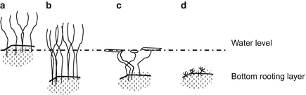

      

      Illustration of emergent macrophytes in a VSB (a) and emergent macrophytes (b), floating macrophytes (c) and submerged macrophytes (d) in a FWS

      • * Emergent (e.g., Bullrush, Common reed, Cattail)

      • * Floating (e.g., Water lily, Duckweed, Water hyacinth)

      • * Submerged (e.g., Pondweed, American shoreweed)

    • ○ Woody species

      • * Shrubs and trees (e.g., willow trees)

  • • Adaptation of vegetation in a constructed wetland

    • ○ As constructed wetlands are started up, conditions evolve due to the fact that the influent is wastewater (Table 10.3)

      Table 10.3 Wetland characteristics and conditions imposed by wastewater influent

      • * Vegetation must adapt to these conditions

• ■ Hydrology and hydraulics in a constructed wetland

  • • Hydrology and hydraulics determine the:

    • ○ Ability of the wetland to handle the design daily flow without backup or surface overflows

    • ○ Achievement of flow conditions that approximate a plug-flow regime without short-circuiting

    • ○ Hydraulic retention time and conditions for removal processes to function and produce a desired effluent quality

  • • To achieve the treatment performance potential of a constructed wetland…

    • ○ It is critical that design provides for, and operation maintains, the desired hydrology and hydraulic conditions

  • • In horizontal flow wetlands—both FWS and VSB designs—the hydraulics are generally determined by key features:

    • ○ Geometry of the wetland

      • * Surface area

      • * Aspect ratio (length to width)

      • * Water depth (Note: typically 1–5 ft (higher end in FWS))

    • ○ Hydraulic gradient from inlet to outlet

    • ○ Flow controls

      • * Inlet and outlet design

      • * Internal flow controls

  • • In addition, for horizontal flow in a VSB wetland

    • ○ Hydraulics can also be determined by the saturated hydraulic conductivity (K_S) of the clean porous media used and the decline from K_S that occurs due to operation (Eq. 10.2, Fig. 10.7)

      Fig. 10.7

      

      Cross section of a vegetated subsurface bed wetland which has a capacity for flow

    • $$ {\mathrm{Q}}_{\mathrm{C}}=\left({\mathrm{K}}_{\mathrm{E}}\right)\left(\mathrm{S}\right)\left({\mathrm{A}}_{\mathrm{xc}}\right) $$

      (10.2)

      Where:

      Q_C = flow through the wetland (gal/day)

      K_E = effective saturated hydraulic conductivity of porous media (gal/day/ft²)

         K_E equals the operational conductivity which is a fraction of K_S

      S = hydraulic gradient of water surface from inlet to outlet (–)

      A_xc = cross-sectional area through which flow occurs (ft²)

  • • The hydraulic effects of vegetation growth and pore clogging

    • ○ Vegetation growth

      • * Leads to root networks and plant parts that can occupy space and reduce hydraulic capacity

    • ○ Pore clogging

      • * Shorter-term processes

        • – Establishment of plant root networks within pores

        • – Filtration of TSS and development of microbial biomass

      • * Longer-term processes

        • – Deposition of inert (mineral) suspended solids

        • – Accumulation of refractory organic materials

        • – Formation of chemical precipitates

    • ○ Hydraulic effects due to vegetation and pore clogging are most important to the function of VSB wetlands (Fig. 10.8) and much less so for FWS wetlands

      Fig. 10.8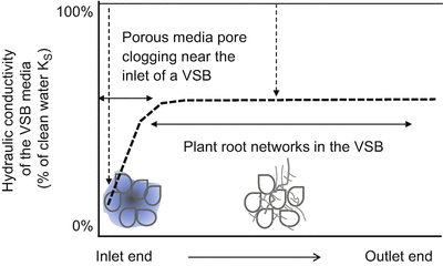

      

      Illustration of how the hydraulic conductivity of the media in a VSB constructed wetland can change from inlet to outlet due to clogging and vegetation (as a percentage of the pre-startup K_S)

    • ○ Effective hydraulic conductivity is used for VSB design

      • * The effective hydraulic conductivity for VSB design (K_E) accounts for clogging processes

      • * Clogging within the inlet zone of a VSB

        • – If the hydraulic capacity declines below the daily loading rate, the inlet of a VSB can become saturated and ponding may occur

          • – Influent that ponds at the inlet can re-infiltrate into the porous media within the VSB a short distance away from the inlet

          • This may or may not be viewed as an unacceptable condition

      • * Clogging within the treatment zone of a VSB

        • – Clogging by vegetation growth can occur but plant decay can yield a stable condition where K_E can be about 50 % of the K_S

      • ○ Choosing a K_E for design of a VSB?

        • – USEPA (2002) recommends setting K_E = 1 % of K_S in the initial 30 % and K_E  = 10 % in the balance of the treatment zone

        • – Jenssen (2015) recommends using an overall value of K_E = 50 % of K_S for sizing of VSBs used for residential applications

• ■ Redox zones within a constructed wetland

  • • Constructed wetlands can have regions or zones that are aerobic, anoxic, or even anaerobic

    • ○ Dissolved oxygen sources and sinks determine redox conditions (Table 10.4)

      Table 10.4 Wetland processes and their effects on dissolved oxygen levels^a

• ■ Water temperatures in a constructed wetland

  • • Temperature is important since it can influence the rates of bioprocesses, the rate of evaporative loss, and water freezing

  • • Wetland water temperatures depend on local climate conditions

    • ○ Daily cycles can be up to 8–10 °C in warm months

    • ○ Annual cycles

      • * In mild to warm climate conditions

        • – Summer maximum and winter minimum

        • – Wetland water temperatures approximate the mean daily air temperatures (under moderate humidity and air temperature)

      • * In cold climate conditions

        • – During winter periods, ice can develop

        • – Ice as well as snow and mulch can help insulate water in the wetland from freezing

        • – However, under-ice water temperatures can be reduced as low as the 1–2 °C range

• ■ Animals and insects in constructed wetlands

  • • Animals and insects can inhabit or visit a constructed wetland

    • ○ The types of animals and insects will be much the same as those that inhabit or visit a natural wetland in the same location

    • ○ Some animals and insects are desirable (e.g., deer, birds, beetles) but others are often not (e.g., snakes, rodents, mosquitos)

    • ○ Constructed wetland design and operation can influence to some extent, whether the animals and insects that inhabit it will be a positive or negative attribute

  • • For VSB constructed wetlands

    • ○ The biggest problems tend to occur in locations where there are undesirable animals (e.g., poisonous snakes, nasty rodents) in the natural environment that can also inhabit and thrive in a VSB wetland

      • * This situation is difficult if not impossible to control through VSB design and operation

  • • For FWS constructed wetlands

    • ○ In some FWS wetlands there can be undesirable animals (e.g., poisonous snakes and dangerous reptiles) and noxious insects, most notably mosquitos

    • ○ Mosquitos will inhabit most FWS wetlands but their numbers can be controlled by design and operation

      • * Control larvae generation that yields mosquitos

      • * Need to foster predator access to larvae

        • – Increase open and deep pool water areas

        • – Avoid large monotypic stands of emergent vegetation

        • – Add birdhouses

    • ○ However, in many situations it is difficult to design and operate a FWS wetland so that it is mosquito-free

      • * An achievable goal? Minimize mosquito production so it is similar to natural wetlands in the same location

10.1.1.4 10-4. Design and Implementation

• ■ Considerations for design and implementation (D&I) of a constructed wetland to achieve secondary treatment and partial nutrient removal or tertiary polishing

  • • Wetland type features and suitability for a particular project

  • • Wastewater source and treatment prior to the wetland

  • • Wetland surface area sizing to handle the daily flow

    • ○ Use of loading specifications

    • ○ Use of modeling techniques

    • ○ Use of a combination of the two

  • • Wetland geometry, porous media, flow controls, and other construction details

  • • Wetland establishment and startup

  • • Wetland O&M

• ■ D&I considerations—Constructed wetland type

  • • FWS and VSB constructed wetlands have different features (Table 10.1) that lend one or the other to particular project applications (Table 10.5)

    Table 10.5 Applications of FWS versus VSB constructed treatment wetlands

• ■ D&I considerations—Wastewater source and treatment prior to the wetland

  • • Wastewaters from varied sources can be treated

    • ○ e.g., graywater, residential wastewater, commercial wastewater

  • • Treatment prior to a wetland

    • ○ The influent to a FWS is typically secondary effluent

      • * e.g., nitrified effluent from an aerobic treatment unit

    • ○ The influent to a VSB is typically primary effluent

      • * e.g., effluent from a septic tank or sedimentation basin

      • * Secondary effluents can also be polished in a VSB wetland

  • • Delivery of influent to a wetland

    • ○ Influent can be delivered to the inlet end of a wetland by gravity flow or through pressurized delivery

• ■ D&I considerations—Wetland surface area required

  • • Wetlands need to be sized with sufficient surface area so they can achieve treatment of one or more constituents of concern

    • ○ For example, produce an effluent with BOD and TSS ≤ 30 mg/L

  • • Surface area sizing is primarily based on

    • ○ Design hydraulic loading rate (HLR_D)

    • ○ Organic loading rate (OLR) limits

  • • Approaches for wetland area sizing

    • ○ Different approaches have been used for surface area sizing of different types of wetlands

    • ○ Two common approaches for sizing are discussed in this section

      • * Area sizing using empirical data from past experiences

      • * Area sizing using modeling of constituent removals

  • • Wetland area sizing—Areal Loading Rates (ALRs)

    • ○ Based on experience, a maximum loading rate per unit of wetland surface area can be specified that is expected to yield a certain effluent quality

      • * For example, for a VSB wetland to achieve an effluent BOD = 20 mg/L, one ALR is ≤0.33 lb-BOD/day/1000 ft²

    • ○ The ALR method is similar to the approach used for sizing oxidation ponds, lagoons, and land treatment units

    • ○ The ALR method works reasonably well for design of wetlands to yield a given effluent BOD₅ and TSS, such as:

      • * BOD and TSS = 30 mg/L

      • * BOD and TSS <20 mg/L and some nutrient removal

    • ○ Example ALR values prescribed to achieve a given effluent quality with respect to BOD or TSS are shown in Table 10.6

      Table 10.6 Areal loading rates to achieve different effluent qualities (after USEPA 2002)

      • * ALRs are based on the entire wetland horizontal surface area

    • ○ For an ALR design the wetland surface area (Fig. 10.9) is calculated using Eq. 10.3

      $$ {\mathrm{A}}_{\mathrm{w}}=\frac{\left({\mathrm{Q}}_{\mathrm{D}}\right)\left({\mathrm{C}}_{\mathrm{I}}\right)\left(\mathrm{F}\right)}{\left(\mathrm{A}\mathrm{L}\mathrm{R}\right)} $$

      (10.3)

      Fig. 10.9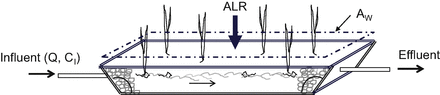

      

      Illustration of the wetland surface area determined by loading rate sizing

      Where:

      A_W = total surface area of the wetland (L × W) (ft²)

      ALR = areal loading rate for a constituent (e.g., BOD) (lb/day/ft²)

      C_I = influent concentration (mg/L)

      Q_D = design daily flow rate (gal/day)

      F = 8.34 × 10⁻⁶ = conversion factor for mg/L to lb/gal

  • • Wetland area sizing—Modeling of constituent removals

    • ○ Constituent removal in a wetland can be modeled assuming reactions are occurring during plug-flow like water movement

      • * A plug-flow like regime can be simulated using a number of continuously stirred tank reactors in series (Fig. 10.10)

        Fig. 10.10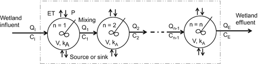

        

        Illustration of a mathematical representation of a pseudo plug-flow regime through a constructed wetland using multiple continuously stirred tank reactors in series

      • * Modeling can account for hydraulic inefficiencies and changes in reaction rate constants with distance in the wetland

    • ○ The P-k_A-C* modeling approach is discussed in this section

    • ○ The P-k_A-C* modeling method accounts for a departure from true plug flow due to hydraulic inefficiencies plus a declining reaction rate constant with distance from the inlet to the outlet in the wetland

      • * Steps in determining the wetland surface area required^a

        • – Select concentration(s) in the influent to the wetland and appropriate background concentrations

        • – Choose target effluent concentrations (e.g., BOD = 20 mg/L)

        • – Analyze potential water balance additions or deletions to flow

          • (inflow and seepage, rain and evapotranspiration)

        • • – Select rate constants and consider temperature effects

          • – Select hydraulic efficiency values (e.g., P-values)

        • – Calculate the areal hydraulic loading rate and the resulting wetland surface area required

        • – Choose other sizing parameters (water depth, geometry, etc.)

        • – Iterate as necessary until effluent concentrations are met

        • – Consider constraints, if any, such as growth cycles, biogeochemical cycles, etc.

          ^aBased on methods in Kadlec and Wallace (2009).

    • ○ In the P-k_A-C* modeling method, Eq. 10.4 can be used to determine an area-based loading rate, q

      $$ \left(\frac{\mathrm{C}-\mathrm{C}*}{{\mathrm{C}}_{\mathrm{I}}-\mathrm{C}*}\right)={\left(1+\frac{{\mathrm{k}}_{\mathrm{A}}\mathrm{y}}{\mathrm{Pq}}\right)}^{-\mathrm{P}} $$

      (10.4)

      Where:

      C = concentration of a constituent at the outlet or a fractional distance from the inlet, y (mg/L)

      C_I = inlet concentration of a constituent (mg/L)

      C* = background concentration of a constituent (mg/L)

      k_A = first-order area-based rate constant (ft/day)

      P = apparent no. of tanks in series for modeling that varies by constituent to account for weathering based on field data (–)

      q = area-based design hydraulic loading rate (HLR) (ft/day or ft³/ft²/day)

      y = fractional distance from the inlet to outlet, unitless (for effluent, y = 1.0)

      ○ Tables 10.7 and 10.8 list input parameter values for P-k_A-C* modeling of FWS and VSB wetlands, respectively

      Table 10.7 P-k_A-C* values for modeling of FWS wetlands (after Kadlec and Wallace 2009)

      Table 10.8 P-k_A-C* values for modeling of VSB wetlands (after Kadlec and Wallace 2009)

    • ○ Equation 10.4 can be rearranged to solve for the area-based HLR to yield a certain pollutant removal (Eq. 10.5)

      $$ \mathrm{q}=\frac{{\mathrm{k}}_{\mathrm{A}}\mathrm{y}}{\mathrm{P}\left[{\left(\frac{1}{\left(\mathrm{C}-\mathrm{C}*\right)/\left({\mathrm{C}}_{\mathrm{I}}-\mathrm{C}*\right)}\right)}^{1/\mathrm{P}}-1\right]} $$

      (10.5)

    • ○ The required wetland surface area can be determined from the calculated area-based hydraulic loading rate using Eq. 10.6

      $$ {\mathrm{A}}_{\mathrm{W}}=\frac{{\mathrm{Q}}_{\mathrm{D}}}{\mathrm{q}} $$

      (10.6)

      Where:

      A_W = wetland surface area (wetted land area) (ft²)

      Q_D = design flow rate (ft³/day)

      q = area-based hydraulic loading rate (HLR) (ft/day)

  • • Other considerations in modeling for wetland area sizing

    • ○ Water balance effects

      • * In some situations, water gains and losses will be important to consider during wetland sizing

        • – Primary water gain is due to precipitation (P)

        • – Primary water losses are due to evapotranspiration (ET)

      • * For sizing, P and ET can be factored into the calculations made using a modeling approach (e.g., by changing Q within one or more tanks in series)

    • ○ Temperature effects

      • * Biological processes and transformation rates can be temperature dependent

        • – Rates can be adjusted for temperature using an appropriate temperature correction factor, θ

      • * For some processes, low or high temperatures can inhibit reactions

        • – For example, the nitrification process can be greatly retarded or cease at temperatures below 10 °C

      • * A common formulation to correct for the temperature effects on biological processes is shown in Eq. 10.7

        $$ {\mathrm{k}}_{\mathrm{T}}={\mathrm{k}}_{20}{\uptheta}^{\left(\mathrm{T}-20\right)} $$

        (10.7)

        Where:

        k_T = reaction rate at T °C (days⁻¹)

        k₂₀ = reaction rate at 20 °C (days⁻¹)

        T = temperature (°C)

        θ = temperature activity coefficient (–)

         Note: In activated sludge biological systems, θ for BOD removal can be about 1.02–1.06 and some adopt values in this range for use with constructed wetlands. However, for constructed wetlands there is evidence that θ for BOD removal may be closer to 1.0. For constituents other than BOD, θ can vary widely (e.g., see Tables 10.7 and 10.8)

  • • Wetland area sizing —Checking the organic loading rate

    • ○ OLR is limited to avoid anaerobic conditions and minimize odors

      • * Maximum OLRs depend on wetland type and the targeted effluent quality as shown in Table 10.9

        Table 10.9 Organic loading rate limits (lb-BOD/day/1000 ft²) for constructed wetlands

      • * For A_W determined by the P-k_A-C* method, the OLR can be checked using Eq. 10.8

        $$ \mathrm{O}\mathrm{L}\mathrm{R}=\frac{\left({\mathrm{Q}}_{\mathrm{D}}\right)\left({\mathrm{BOD}}_5\right)\left(\mathrm{F}\right)}{{\mathrm{A}}_{\mathrm{W}}\hbox{'}} $$

        (10.8)

        Where:

        OLR = organic loading rate (lb-BOD₅/day/ft²)

        For guidance on maximum rates see Table 10.9

        Q_D = design daily flow (gal/day)

        BOD₅ = Influent BOD₅ (mg/L)

        A_W′ = wetland surface area actually provided based on the chosen geometry (L × W) (ft²)

        F = 8.34 × 10⁻⁶ = conversion factor for mg/L to lb/gal

• ■ D&I considerations—Water depth and rooting depth

  • • In a VSB wetland (Fig. 10.11a)

    Fig. 10.11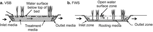

    

    Illustration of water depth and rooting bed depth in constructed wetlands

    • ○ Typical porous media depths are 1.5–2.5 ft to provide for rooting and horizontal water flow

    • ○ The water surface is normally 0.25–0.5 ft below the bed surface

  • • In a FWS wetland (Fig. 10.11b)

    • ○ Some depth of media is required for rooting plants (e.g., 1 ft)

    • ○ Water depths in the inlet and outlet zones are often 2–3 ft while the open water surface zone is 4–5 ft

  • • Relationship of water depth to treatment efficiency

    • ○ For a wetland design based on areal loading rates

      • * R_E is based on the areal loading rate and not directly related to HRT (Fig. 10.12)

        Fig. 10.12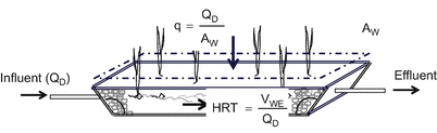

        

        Relationship of design hydraulic parameters in a VSB wetland

    • ○ For a wetland design based on modeling with area-based reaction rates where q = Q_D/A_W and R_E is not affected by the HRT

      • * For a given Q_D, q does not change with increases in depth

    • ○ Thus, increasing water depth alone would not be predicted to increase R_E

• ■ D&I considerations—Wetland volume and HRT

  • • Wetland volume

    • ○ The nominal volume of a wetland is equal to the bulk volume of the wetland defined by the area and water depth (Eq. 10.9)

      $$ {\mathrm{V}}_{\mathrm{N}}=\left({\mathrm{A}}_{\mathrm{W}}\right)\left({\mathrm{d}}_{\mathrm{W}}\right) $$

      (10.9)

    • ○ The water-filled volume accounts for the presence of gravel or plants as given by Eq. 10.10

      $$ {\mathrm{V}}_{\mathrm{W}}=\left(\upvarepsilon \right){\mathrm{V}}_{\mathrm{N}} $$

      (10.10)

      Where:

      V_N = nominal wetland volume is the bulk volume = L × W × d_W (ft³)

      V_W = water volume equals the open porosity in the wetland media (ft³)

      A_W = wetland surface area (ft²)

      d_W = water depth (ft)

      ε = porosity of clean gravel (other similar media) in a VSB (ft³/ft³)

       =plant-based void ratio in a FWS (ft³/ft³)

    • ○ Some designers consider an effective water volume that accounts for the presence of gravel or plants plus inactive flow zones using Eqs. 10.11 and 10.12

      $$ {\mathrm{V}}_{\mathrm{WE}}=\left({\mathrm{e}}_{\mathrm{V}}\right)\left(\upvarepsilon \right){\mathrm{V}}_{\mathrm{N}} $$

      (10.11)
      $$ {\mathrm{e}}_{\mathrm{V}}=\left(\frac{{\mathrm{V}}_{\mathrm{A}}}{{\mathrm{V}}_{\mathrm{B}}}\right) $$

      (10.12)

      Where:

      V_B = bulk volume of the wetland = L × W × d_W (ft³)

      V_WE = effective water volume accounting for porosity and inactive zones (ft³)

      V_A = volume of wetland containing water active in flow (ft³)

      A_W = wetland surface area (ft²)

      d_W = water depth (ft)

      ε = porosity of clean gravel in a VSB (ft³/ft³) (often assumed 0.40)

       =plant-based void ratio in a FWS (reported as 0.65–0.75)

      e_V = wetland volumetric efficiency accounting for inactive flow zones (–) (reported as FWS = 0.82, VSB = 0.83)^a

      ^a Source: Kadlec and Wallace (2009)

  • • Wetland hydraulic retention time

    • ○ With the wetland volume determined, the hydraulic retention time can be calculated using Eqs. 10.13 and 10.14

      $$ {\mathrm{HRT}}_{\mathrm{N}}=\frac{{\mathrm{V}}_{\mathrm{N}}}{\mathrm{Q}} $$

      (10.13)
      $$ {\mathrm{HRT}}_{\mathrm{E}}=\frac{{\mathrm{V}}_{\mathrm{WE}}}{\mathrm{Q}} $$

      (10.14)

      Where:

      HRT_N = nominal hydraulic retention time (days)

      HRT_E = effective hydraulic retention time (days)

      V_N = nominal wetland volume is the bulk volume = L × W × d_W (ft³)

      V_WE = effective water volume accounting for porosity plus inactive flow zones (ft³)

      Q = flow rate through the wetland—design or actual (ft³/day)

• ■ D&I considerations—Wetland porous media

  • • A description of flow zones is presented in Table 10.10 and a summary of the media size ranges used is given in Table 10.11

    Table 10.10 Features of key flow zones within a VSB constructed wetland

    Table 10.11 Characteristics of porous media used in VSB wetlands (after Knowles et al. 2011)

• ■ D&I considerations—Flow rate capacity of a VSB

  • • Flow rate capacity is controlled by the cross-sectional area of the wetland (A_XC) and K_E of the porous media after accounting for hydraulic conductivity loss during operation (Fig. 10.13)

    Fig. 10.13

    

    Example approach to cross-sectional area sizing within a VSB wetland

  • • A minimum A_XC is required so the VSB can handle the daily flow without surfacing of water flowing through it

  • • The minimum cross-sectional area required can be calculated using Eq. 10.15

    • $$ {\mathrm{A}}_{\mathrm{XC}}=\left({\mathrm{d}}_{\mathrm{W}}\right)\left(\mathrm{W}\right)=\frac{{\mathrm{Q}}_{\mathrm{D}}}{\left({\mathrm{K}}_{\mathrm{S}}\right)\left(\mathrm{F}\right)\left(\mathrm{S}\right)} $$

      (10.15)

      Where:

      A_XC = cross-sectional area of the wetland required for Q_D (ft²)

      d_W = depth of water in the wetland (ft)

      W = width of the wetland (ft)

      Q_D = design flow rate (ft³/day)

      K_S = saturated hydraulic conductivity of the clean VSB media (ft/day)

      F = factor to account for loss in K_S due to clogging (Note: (K_S)(F) = K_E) (USEPA (2002) recommends F = 0.01 for the initial 30 % of the treatment zone and 0.10 for the balance of that zone; Jenssen (2015) recommends F = 0.50 for the overall treatment zone)

      S = hydraulic gradient from the inlet to outlet (slope) (ft/ft) (If the VSB bottom is sloped, can use that as S (typ. ≤0.01) For flat bottoms with outlet control use S ≈ 0.001)

    • ○ Hydraulic conductivity properties of porous media used within the treatment zone of a VSB wetland

      • * Table 10.12 shows example media with hydraulic properties and the flow rate capacities per unit of A_XC based on K_E = 10 or 50 % of K_S

        Table 10.12 Hydraulic conductivity properties of porous media used in VSB wetlands

• ■ D&I considerations—Wetland surface area geometry

  • • The length (L) and width (W) can be selected to help achieve plug-flow like conditions and avoid short-circuiting

    • ○ L:W ratios of 1:1 to 4:1 are generally desirable

      • * L:W ratios apply to the entire wetland or individual cells within it if flow control boundaries are used (Fig. 10.14)

        Fig. 10.14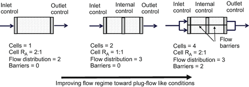

        

        Illustration of geometries, cell aspect ratios, and internal flow control structures to enhance plug-flow conditions (Note: The wetland A_W is the same for all three configurations)

    • ○ Length and width can yield a desired aspect ratio (R_A) (Eq. 10.16)

      $$ {\mathrm{R}}_{\mathrm{A}}=\frac{\mathrm{L}}{\mathrm{W}} $$

      (10.16)

      Where:

      W = width of the wetland or a cell within it (ft)

      W has to be sufficient so the cross-sectional area (A_XC = W × d_w) is ≥the size needed to handle Q_D (Eq. 10.15); but limited to avoid short circuiting (e.g., W ≤ 200 ft)

      L = length of the wetland or a cell within it (ft)

      R_A = aspect ratio, length to width of the wetland or cell within it (e.g., 1:1 to 4:1)

  • • Flow controls can be used to improve wetland hydraulics

    • ○ Vertical flow controls can be used to divide the wetland into cells (Fig. 10.14)

      • * Horizontal flow controls can be used if density driven flow is of concern

    • ○ Illustration of a potential solution for a wetland area that has a high A_XC needed to handle Q_D (as calculated using Eq. 10.15)

      • * Dividing the wetland into four parallel that provide the same total A_XC but have better L:W ratios (Fig. 10.15)

        Fig. 10.15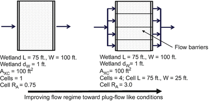

        

        Illustration of an approach to provide the same wetland A_W and A_XC but with improved flow regime characteristics

• ■ D&I considerations—Installation at the site

  • • Establishment of a constructed wetland includes the physical design, construction, and vegetation planting

  • • Wetland location on a site must account for constraints such as:

    • ○ Ensuring construction equipment access

    • ○ Choosing sites with gentle slopes (1–3 % are easiest)

    • ○ Avoiding damage to existing utilities

    • ○ Floodplains vs. floodways—avoid

    • ○ Compliance with applicable regulations and permitting processes

  • • Layout and configuration of the wetland

    • ○ Number of independent wetland flow paths (e.g., ≥2 for larger design flows and wetland sizes)

    • ○ Wetland area geometry and flow controls for cell configurations

  • • Bed containment and bed depth

    • ○ Containment

      • * Synthetic liners

        • – For small projects (e.g., <1000 ft²), one-piece factory seamed PVC liners (0.76 mm thick) can be used

        • – For larger projects, high density polyethylene (1.1–1.5 mm thick) can be used with in-field welded seams after placement

      • * Natural liners

        • – In some applications, compacted soil (with high clay content) might be used

    • ○ Bed depth

      • * FWS require bed depth for rooting (e.g., 1 ft) and additional water column depth for flow (e.g., 2–3 ft in the inlet and outlet zones and 4–5 ft in the open water zone)

      • * VSB wetlands need depth for rooting and flow (e.g., 2 ft)

  • • Water flow controls

    • ○ Inlet structures (Fig. 10.16)

      Fig. 10.16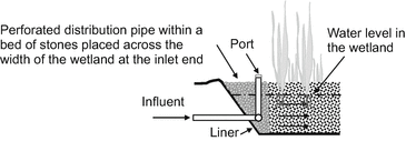

      

      Cross section of an example inlet configuration

      • * Designed to achieve distribution of the influent across the entire A_XC of the wetland inlet zone

      • * Uniform distribution across the inlet Is very important to achieving plug-flow like hydraulics, which are needed for high treatment efficiency

      • * Inlets can be made with piping, channels, chambers, and coarse rock beds

    • ○ Outlet structures and water level controls (Fig. 10.17)

      Fig. 10.17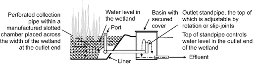

      

      Cross section of an example of an outlet and water level control configuration 10.63

      • * Outlet design is very important to wetland hydraulics to:

        • – Enhance plug-flow regime through the wetland

        • – Avoid short-circuiting and inactive flow zones

        • – Enable control of the water level in the wetland

      • * Outlets can be made with piping, rock channels, chambers, and combinations thereof

      • * Water level controls can be implemented in the body of the wetland or in a separate basin near the outlet end

    • ○ Photographs of a VSB inlet and outlet are shown in Fig. 10.18

      Fig. 10.18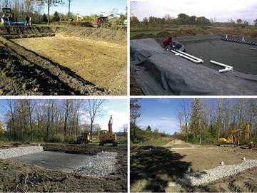

      

      Photographs of a VSB wetland during construction (Source: www.goshen.edu/merrylea/collegiate/riethvillage.html)10.64

  • • Vegetation establishment

    • ○ Plant selection

      • * Select plants that are locally available and are noninvasive species

      • * Plants must be suited to the climate and wetland environment with consideration of aesthetic values

    • ○ Planting

      • * Cuttings (e.g., 4-in. long) or potted plants are placed about 2 in. into the porous media

      • * For most common species, spacing is on the order of 20–60 plants per 100 ft²

    • ○ Initiating growth

      • * The wetland zone is flooded with water to initiate growth

    • ○ Figure 10.19 presents a photograph of a newly planted subsurface vegetated bed wetland.

      Fig. 10.19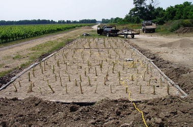

      

      Photograph of a newly planted VSB wetland

• ■ D&I considerations—Wetland startup

  • • Once a wetland is established and started up it can take time to achieve stable performance with respect to treatment efficiency

  • • Startup can occur relatively quickly with VSBs

    • ○ Biological processes that occur in biofilms that develop during flow through porous media that are not dependent on plants

  • • Startup for FWS wetlands can take longer

    • ○ For FWS wetlands, stable performance can take up to 1–2 growing seasons

• ■ D&I considerations—Operation and maintenance

  • • After startup, routine operation of a constructed wetland is typically minimal, and might include:

    • ○ Flow monitoring and adjustments as needed

    • ○ Inspection of inlets and outlets as well as berms

    • ○ Need for monitoring of effluent quality varies widely

      • * Depends on discharge plans and regulatory requirements

  • • Maintenance functions in a properly designed and implemented wetland can include:

    • ○ Harvesting of plants (required for true removal of constituent uptake)

    • ○ Solids removal in FWS wetlands (possibly only every 10–15 years)

    • ○ Recovering from clogging in VSB wetlands (possibly only every 20 years±)

10.1.1.5 10-5. Summary

• ■ Constructed wetlands exploit natural wetland processes to treat wastewaters and other impaired waters

  • • FWS wetlands utilize horizontal flow through a shallow pond planted with floating, submerged or emergent vegetation

    • ○ Often used for tertiary polishing of secondary effluents

  • • VSB wetlands utilize subsurface flow through a bed of porous media that is planted with emergent vegetation

    • ○ Often used for secondary treatment of primary effluents

• ■ Constructed wetland design and implementation

  • • Constructed wetlands can produce a high quality effluent and potentially provide wildlife habitat and aesthetic benefits

  • • Wetlands can be passive and not require power or chemicals

  • • Constructed wetlands can be implemented in a wide range of conditions, including very cold and very hot climates

  • • Wetlands do require land area and time for startup

10.1.1.6 10-6. Example Problems

• ■ 10EP-1. Adjusting a total nitrogen removal rate constant for temperature

  • • Given information

    • ○ The wetland type is a free water surface wetland that is being designed using a P-k_A-C* modeling approach

    • ○ A removal rate constant is needed for the wetland that will be located in a climate with an average temperature of 12 °C

  • • Determine

    • ○ Calculate the k_A for a wetland that is operated at 12 °C

  • • Solution

    • ○ Based on literature data, select a k_A value for total N removal = 0.11 ft/day at 20 °C with a θ = 0.156 (e.g., see Table 10.7)

    • ○ Using Eq. 10.7, adjust the k_A at 20 °C to k_A at 12 °C

      $$ \begin{array}{l}{\mathrm{k}}_{\mathrm{T}}={\mathrm{k}}_{20}{\uptheta}^{\left(\mathrm{T}-20\right)}={\mathrm{k}}_{20}{1.056}^{\left(12-20\right)}\\ {}{\mathrm{k}}_{12}={\mathrm{k}}_{20}(0.647)\\ {}{\mathrm{k}}_{12}=0.11(0.647)=0.071\;\mathrm{ft}/\mathrm{d}\end{array} $$

      (10.7)

• ■ 10EP-2. Sizing a VSB constructed wetland

  • • Given information

    • ○ Design daily flow = 10,000 gal/day from an apartment complex

    • ○ Treatment prior to the wetland is by a septic tank unit w/ screen (STE BOD₅ = 150 mg/L, TSS = 40 mg/L, NH₄ ⁺-N = 40 mg-N/L)

    • ○ Wetland temperature is relatively constant at 10 °C

    • ○ Treatment goal: reduce the STE BOD₅ to 30 mg/L (after accounting for internally produced BOD)

    • ○ VSB treatment zone = 20–30 mm diameter gravel (ε = 0.40, K_S = 32,800 ft/day, F = 0.1). VSB bed depth = 1.5 ft with a water depth = 1 ft and a VSB hydraulic gradient = 0.5 %

  • • Determine

    • ○ Using ALR and P-k_A-C* methods, determine the wetland surface area (ft²), hydraulic retention time (days), and wetland volume (ft³)

  • • Solution

    • ○ VSB wetland area based on ALR loading specifications

      $$ \begin{array}{c}{\mathrm{A}}_{\mathrm{W}}=\frac{\left({\mathrm{Q}}_{\mathrm{D}}\right)\left({\mathrm{C}}_{\mathrm{I}}\right)\left(\mathrm{F}\right)}{\left(\mathrm{A}\mathrm{L}\mathrm{R}\right)}\hfill \\ {}{\mathrm{A}}_{\mathrm{W}}=\frac{\left(10,\kern-1pt 000\kern0.5em \mathrm{gal}/\mathrm{d}\right)\left(150\;\mathrm{mg}/\mathrm{L}\right)\left(8.34\times {10}^{-6}\right)}{1.23\kern0.5em \mathrm{lb}/\mathrm{d}\mathrm{ay}/1000{\mathrm{ft}}^2}\\ {}\mathrm{A}\mathrm{L}\mathrm{R}\ {\mathrm{A}}_{\mathrm{W}}=10,\kern-1pt 170\kern0.5em {\mathrm{ft}}^2\hfill \end{array} $$

      (10.3)

    • ○ Wetland area based on P-k_A-C* modeling

      • * Calculate the areal hydraulic loading rate, q

        $$ \begin{array}{l}\mathrm{q}=\frac{{\mathrm{k}}_{\mathrm{A}}\mathrm{y}}{\mathrm{P}\left[{\left(\frac{1}{\left(\mathrm{C}-\mathrm{C}*\right)/\left({\mathrm{C}}_{\mathrm{I}}-\mathrm{C}*\right)}\right)}^{1/\mathrm{P}}-1\right]}\\ {}\mathrm{q}=\frac{(0.22)(1)}{3\left[{\left(\frac{1}{\left(30-10\right)/\left(150-10\right)}\right)}^{1/3}-1\right]}\\ {}\mathrm{q}=\frac{0.22}{2.74}=0.08\kern0.5em \mathrm{ft}/\mathrm{day}\end{array} $$

        (10.5)

      • * Calculate the wetland surface area (A_w) using the calculated hydraulic loading rate (q) and the design daily flow rate (Q_D)

        $$ \begin{array}{c}{\mathrm{A}}_{\mathrm{W}}=\frac{{\mathrm{Q}}_{\mathrm{D}}}{\mathrm{q}}\\ {}{\mathrm{A}}_{\mathrm{W}}=\frac{1337\kern0.5em {\mathrm{ft}}^3/\mathrm{day}}{0.08\kern0.5em \mathrm{ft}/\mathrm{day}}\\ {}\mathrm{PTIS}\ {\mathrm{A}}_{\mathrm{W}}=16,\kern-1pt 710\kern0.5em {\mathrm{ft}}^2\end{array} $$

        (10.6)

      • * Check to see if the organic loading rate for the A_W determined by P-k_A-C* modeling is acceptable

        $$ \mathrm{O}\mathrm{L}\mathrm{R}=\frac{\left({\mathrm{Q}}_{\mathrm{D}}\right)\left({\mathrm{BOD}}_5\right)\left(\mathrm{F}\right)}{{\mathrm{A}}_{\mathrm{W}}\hbox{'}} $$

        (10.8)
        $$ \begin{array}{l}\mathrm{O}\mathrm{L}\mathrm{R}=\frac{\left({\mathrm{Q}}_{\mathrm{D}}\right)\left({\mathrm{BOD}}_5\right)\left(8.34\times {10}^{-6}\right)}{{\mathrm{A}}_{\mathrm{W}}\hbox{'}}\\ {}\mathrm{O}\mathrm{L}\mathrm{R}=\frac{\left(10,\kern-1.75pt 000\kern0.5em \mathrm{gal}\right)\left(150\kern0.5em \mathrm{mg}\kern0.1em /\kern0.1em \mathrm{L}\right)\left(8.34\times {10}^{-6}\right)}{16,\kern-1.5pt 710{\mathrm{ft}}^2}\\ {}\mathrm{O}\mathrm{L}\mathrm{R}=0.00075\kern0.5em \mathrm{lb}\kern0.6em {\mathrm{BOD}}_5\kern0.1em /\kern0.1em {\mathrm{ft}}^2\\ {}\mathrm{O}\mathrm{L}\mathrm{R}=0.75\kern0.5em \mathrm{lb}\kern0.6em {\mathrm{BOD}}_5/1,\kern-1pt 000\kern0.22em {\mathrm{ft}}^2\end{array} $$

• ✓ This OLR is okay based on a guidance value of 1.23 lb-BOD₅/1000 ft² (refer to Table 10.9)

  • ○ Determine the wetland volume

    • * Nominal volume (V_N) depends on A_W and selected d_W

      $$ {\mathrm{V}}_{\mathrm{N}}=\left({\mathrm{A}}_{\mathrm{W}}\right)\left({\mathrm{d}}_{\mathrm{W}}\right) $$

      (10.9)
      $$ \begin{array}{l}\underline {\mathrm{V}:\kern0.5em \mathrm{A}\mathrm{L}\mathrm{R}\;\mathrm{based}\;{\mathrm{A}}_{\mathrm{W}}}\\ {}{\mathrm{V}}_{\mathrm{N}}=\left({\mathrm{A}}_{\mathrm{w}}\right)\left({\mathrm{d}}_{\mathrm{W}}\right)\\ {}{\mathrm{V}}_{\mathrm{N}}=\left(10170\kern0.5em {\mathrm{ft}}^2\right)\left(1\kern0.5em \mathrm{ft}\right)\\ {}{\mathrm{V}}_{\mathrm{N}}=10,\kern-1.5pt 170\kern0.5em {\mathrm{ft}}^3\\ {}{\mathrm{V}}_{\mathrm{W}\mathrm{E}}=(0.83)(0.4)\left(10,\kern-1.5pt 170\kern0.5em {\mathrm{ft}}^3\right)\\ {}{\mathrm{V}}_{\mathrm{W}\mathrm{E}}=3,\kern-1.5pt 376\kern0.5em {\mathrm{ft}}^3\end{array} $$
      $$ {\mathrm{V}}_{\mathrm{WE}}=\left({\mathrm{e}}_{\mathrm{V}}\right)\left(\upvarepsilon \right){\mathrm{V}}_{\mathrm{N}} $$

      (10.11)
      $$ \begin{array}{l}\underline {\mathrm{V}:\kern0.5em \mathrm{P}-{\mathrm{k}}_{\mathrm{A}}-\mathrm{C}\kern0.1em *\kern0.5em \mathrm{based}\kern0.5em {\mathrm{A}}_{\mathrm{W}}}\\ {}{\mathrm{V}}_{\mathrm{N}}=\left({\mathrm{A}}_{\mathrm{w}}\right)\left({\mathrm{d}}_{\mathrm{W}}\right)\\ {}{\mathrm{V}}_{\mathrm{N}}=\left(16710\kern0.5em {\mathrm{ft}}^2\right)\left(1\kern0.5em \mathrm{ft}\right)\\ {}{\mathrm{V}}_{\mathrm{N}}=16,\kern-1.5pt 710\kern0.5em {\mathrm{ft}}^3\\ {}{\mathrm{V}}_{\mathrm{W}\mathrm{E}}=(0.83)(0.4)\left(16710\kern0.5em {\mathrm{ft}}^3\right)\\ {}{\mathrm{V}}_{\mathrm{W}\mathrm{E}}=5,\kern-1.5pt 540\kern0.5em {\mathrm{ft}}^3\end{array} $$

    • * Effective volume (V_WE) accounts for porosity and inactive flow zones

  • ○ Determine the effective wetland hydraulic retention time (HRT_E)

    • * Nominal HRT_N depends on calculated A_W and selected d_W

    • * Effective HRT_E accounts for porosity and volumetric efficiency

    • * Note Q can be chosen to equal Q_D or the actual daily flow rate

      $$ {\mathrm{HRT}}_{\mathrm{N}}=\frac{{\mathrm{V}}_{\mathrm{N}}}{\mathrm{Q}}\kern1pc (10.13)\kern5pc {\mathrm{HRT}}_{\mathrm{E}}=\frac{{\mathrm{V}}_{\mathrm{WE}}}{\mathrm{Q}} $$

      (10.14)
      $$ \begin{array}{l}\underline {{\mathrm{HRT}}_{\mathrm{E}}:\kern0.5em \mathrm{A}\mathrm{L}\mathrm{R}\kern0.5em \mathrm{based}\kern0.5em {\mathrm{A}}_{\mathrm{W}}}\\ {}{\mathrm{HRT}}_{\mathrm{E}}=\frac{{\mathrm{V}}_{\mathrm{W}\mathrm{E}}}{{\mathrm{Q}}_{\mathrm{D}}}\\ {}{\mathrm{HRT}}_{\mathrm{E}}=\frac{3,\kern-1.5pt 376\kern0.5em {\mathrm{ft}}^3}{1,\kern-1.5pt 337\kern0.5em {\mathrm{ft}}^3\kern0.1em /\kern0.1em \mathrm{day}}=2.5\kern0.5em \mathrm{day}\mathrm{s}\end{array}\begin{array}{l}\underline {{\mathrm{HRT}}_{\mathrm{E}}:\kern0.5em \mathrm{P}-{\mathrm{k}}_{\mathrm{A}}-\mathrm{C}\kern0.1em *\kern0.5em \mathrm{based}\kern0.5em {\mathrm{A}}_{\mathrm{W}}}\\ {}{\mathrm{HRT}}_{\mathrm{E}}=\frac{{\mathrm{V}}_{\mathrm{W}\mathrm{E}}}{{\mathrm{Q}}_{\mathrm{D}}}\\ {}{\mathrm{HRT}}_{\mathrm{E}}=\frac{5,\kern-1.5pt 540\kern0.5em {\mathrm{ft}}^3}{1,\kern-1.5pt 337\kern0.5em {\mathrm{ft}}^3\kern0.1em /\kern0.1em \mathrm{day}}=4.1\kern0.5em \mathrm{day}\mathrm{s}\end{array} $$

  • ○ A comparison of results is shown in Table 10EP.1

    Table 10EP.1 Comparison of a wetland designed using different approaches

  • ○ Some derived values based on the given values and sizing calculations are shown in Table 10EP.2

    Table 10EP.2 Comparison of some derived values based on the results for a wetland designed using different approaches

• ■ 10EP-3. Determining the geometry for a VSB constructed wetland

  • • Given information

    • ○ Design daily flow = 10,000 gal/day (1337 ft³/day)

    • ○ VSB surface area = 13,140 ft²

    • ○ VSB treatment zone = 30 mm diameter gravel (ε = 0.40, clean media K_S = 32,800 ft/day, F = 0.1). VSB bed depth = 2.0 ft with a water-filled depth = 1.5 ft and VSB hydraulic gradient = 0.5 %

  • • Determine

    • ○ The minimum cross-sectional area required to handle the design flow rate and the length and width of the wetland surface area

  • • Solution

    • ○ Calculation of A_XC using Eq. 10.15

      $$ \begin{array}{l}{\mathrm{A}}_{\mathrm{XC}}=\left({\mathrm{d}}_{\mathrm{W}}\right)\left(\mathrm{W}\right)=\frac{{\mathrm{Q}}_{\mathrm{D}}}{\left({\mathrm{K}}_{\mathrm{S}}\right)\left(\mathrm{F}\right)\left(\mathrm{S}\right)}\\ {}{\mathrm{A}}_{\mathrm{XC}}=\frac{1,\kern-1.5pt 337\;{\mathrm{ft}}^3\kern0.1em /\kern0.1em \mathrm{day}}{\left(32,\kern-1.5pt 800\;\mathrm{ft}\kern0.1em /\kern0.2em \mathrm{day}\right)(0.1)(0.005)}\\ {}{\mathrm{A}}_{\mathrm{XC}}=81.5\kern0.5em {\mathrm{ft}}^2\end{array} $$

      (10.15)

    • ○ Calculation of the minimum width needed to handle Q_D

      $$ \begin{array}{l}{\mathrm{A}}_{\mathrm{XC}}=\left({\mathrm{d}}_{\mathrm{W}}\right)\left(\mathrm{W}\right)=81.5\ {\mathrm{ft}}^2\\ {}\mathrm{W}=\frac{81.5\ {\mathrm{ft}}^2}{1\;.5\;\mathrm{ft}}=54.3\kern0.5em \mathrm{ft}\end{array} $$

      (10.15)

    • ○ Calculation of the length based on the minimum width required

      $$ \begin{array}{l}{\mathrm{A}}_{\mathrm{W}}=\mathrm{L}\times \mathrm{W}\\ {}\mathrm{L}=\frac{{\mathrm{A}}_{\mathrm{W}}}{\mathrm{W}}=\frac{13,140\;{\mathrm{ft}}^2}{54.3\;\mathrm{ft}}=242\kern0.5em \mathrm{ft}\end{array} $$

    • ○ Calculate the aspect ratio

      $$ {\mathrm{R}}_{\mathrm{A}}=\frac{\mathrm{L}}{\mathrm{W}}=\frac{242}{54.3}=4.5 $$

      (10.16)

      • * The wetland aspect ratio of 4.5 is fine and within a reasonable range based on engineering practice limits

      • * If the landscape area available required a different wetland geometry the length and width could be adjusted as long as the resulting R_A (with one or more cells) would be conducive to plug-flow like conditions in the wetland

References

References cited in Chap. 10 are listed along with other references that have content relevant to the topics covered in Chap. 10.
Borjesson P, Bends G (2006) The prospects for willow plantations for wastewater treatment in Sweden. Biomass Bioenergy 30:428–438
Colorado Constructed Treatment Wetlands Inventory, Office of Energy Management and Conservation, March 2001
Crites RW, Tchobanoglous G (1998) Small and decentralized wastewater management systems. McGraw-Hill, New York, 1084 pp
Gagnon V, Chazarenc F, Comeau Y, Brisson J (2007) Influence of saprophyte species on microbial density and activity in constructed wetlands. Water Sci Technol 56(3):249–254
ITRC (2003) Technical and regulatory guidance document for constructed treatment wetlands. Interstate Technology and Regulatory Council. 199 pp. http://www.itrcweb.org/Guidance/ListDocuments?topicID=29&subTopicID=41
ITRC (2005) Characterization, design, construction, and monitoring of mitigation wetlands. Interstate Technology and Regulatory Council. 197 pp. http://www.itrcweb.org/Guidance/ListDocuments?topicID = 29&subTopicID = 41
Jenssen PD (2015) Norwegian University of Life Sciences, Ås, Norway. Personal communication. October 27, 2015
Kadlec RH, Wallace SD (2009) Treatment wetlands, 2nd edn. CRC Press, New York, NY, 1016 pp
Knowles P, Dort G, Nivala J, Garcia J (2011) Review of Clogging in subsurface-flow treatment wetlands: occurrence and contributing factors. Ecol Eng 37(2011):99–112
Sanford WE, Steenhuis TS, Parlance JY, Surface JM, Peverly JH (1995) Hydraulic conductivity of gravel and sand as substrates in rock-reed filters. Ecol Eng 4:L321–L336
U.S. Environmental Protection Agency (2000) Constructed wetlands treatment of municipal wastewaters. EPA/625/R-99/010. Office of Research and Development, Cincinnati, OH. 166 pp. http://water.epa.gov/type/wetlands/restore/upload/constructed-wetlands-design-manual.pdf
U.S. Environmental Protection Agency (2002) Onsite wastewater treatment systems manual. EPA/625/R-00/008. http://www.epa.gov/ORD/NRMRL/Pubs/625R00008/625R00008.htm
Vymazal J, Kröpfelová L (2008) Wastewater treatment in constructed wetlands with horizontal sub-surface flow. Springer Science+Business Media B.V., Dordrecht, The Netherlands
WERF (2006) Small-scale constructed wetland treatment systems. WERF Publication No. 01-CTS-5
Author information
Authors and Affiliations