Product Rules and Distributive Laws

Abstract

We give a categorical perspective on various product rules, including Brzozowski’s product rule ($(st)_a = s_a t + o(s) t_a$) and the familiar rule of calculus ($(st)_a = s_a t + s t_a$). It is already known that these product rules can be represented using distributive laws, e.g. via a suitable quotient of a GSOS law. In this paper, we cast these product rules into a general setting where we have two monads S and T, a (possibly copointed) behavioural functor F, a distributive law of T over S, a distributive law of S over F, and a suitably defined distributive law $TF \Rightarrow FST$. We introduce a coherence axiom giving a sufficient and necessary condition for such triples of distributive laws to yield a new distributive law of the composite monad ST over F, allowing us to determinize FST-coalgebras into lifted F coalgebras via a two step process whenever this axiom holds.

J. Winter—This work was supported by the Polish National Science Centre (NCN) grant 2012/07/E/ST6/03026.

These keywords were added by machine and not by the authors. This process is experimental and the keywords may be updated as the learning algorithm improves.

1 Introduction

In [Brz64], Brzozowski introduced a calculus of derivatives for regular expressions, including amongst other rules the product rule

$$\begin{aligned} (xy)_a = x_a y + o(x) y_a \end{aligned}$$

which can be contrasted with the familiar (Leibniz) product rule from calculus (here rephrased with a somewhat uncommon nomenclature, to highlight the correspondences and differences with Brzozowski’s rule)

$$\begin{aligned} (xy)_a = x_a y + x y_a. \end{aligned}$$

In the work of Rutten, starting with [Rut98], a picture started to emerge in which Brzozowski’s calculus of derivatives was absorbed into the framework of universal coalgebra. Notably, in [Rut03, Rut05] both product rules were considered as behavioural differential equations, or coinductive definitions, possessing unique solutions, and defining respectively the convolution product (Brzozowski’s rule) and the shuffle product (Leibniz’ rule) on the final coalgebra.

In the work of Bonsangue and Rutten together with the present author, starting with [WBR11], a coalgebraic presentation of the context-free languages was given, in which Brzozowski’s derivative rules (excluding the star rule) again play a crucial role. This work was based on a concretely presented extension of $2 \times \mathcal {P}_\omega (-^*)^A$-coalgebras into $2 \times -^A$-coalgebras, as in the following diagram:

In [BHKR13], it was shown that the above diagram could be understood in terms of a distributive law of the monad $\mathcal {P}_\omega (-^*)$ over the cofree copointed functor on $2 \times -^A$, that is, over $(- \times (2 \times -^A), \pi _1)$ by means of a suitable quotient of distributive laws. This firmly established the connection between the work of [WBR11] and the general categorical framework of bialgebras and distributive laws, considered in e.g. [LPW00, Bar04, Jac06a, Jac06b, Kli11, JSS12], as well as to the (closely related) generalized powerset construction presented in [SBBR10, SBBR13].

Moreover, in [BRW12], the approach was generalized from formal languages to formal power series, thus giving a coalgebraic characterization of the constructively algebraic power series.

In [Win14], the author’s Ph.D. thesis, this extension was broken up into a two step process, as in the diagram,

and it was noted that the first extension corresponded directly to the product rule (combined with the unit rule), whereas the second extension was simply an instance of ordinary determinization, applied to a coalgebra which is by itself infinite. This two-step process again easily generalizes from the setting of languages to the setting of noncommuting power series over commutative semirings; however, no general categorical presentation of this two-step process was given in the thesis.

The main aim of this paper is to give such a categorical presentation of this two-step process. This involves a setting including both distributive laws between monads $\lambda ^0: TS \Rightarrow ST$, distributive laws of a monad over a functor (or copointed functor) $\lambda ^2: SF \Rightarrow FS$, as well as a, suitably defined, distributive law of type $\lambda ^1: TF \Rightarrow FST$ (this definition will be given in Sect. 3).

In Sect. 4, we will present our main result, which states that the three laws as suggested above can be combined to form a new distributive law $\hat{\lambda }$ of the composite monad ST over F, if and only if a certain coherence axiom involving the three laws is satisfied. This construction works regardless whether F is an ordinary or copointed functor. The proof that satisfaction of the coherence axiom implies the multiplicative law of the distributive law of the composite monad ST over F was automatically derived using a Prolog program written for this purpose.

We then show that both the Brzozowski and Leibniz product rules, as well as the (simpler) pointwise rule defining the Hadamard product, can be cast into this setting, and that the coherence axiom is satisfied in these cases, and additionally present a counterexample where the coherence axiom is not satisfied. We conclude with a presentation of an extension of the generalized powerset construction to incorporate these two-step extensions.

Related work. All of the aforementioned references can be regarded as related work. In particular, [Che07] gives a similar coherence condition, for the existence of composite distributive laws in the context of distributive laws between monads. The relationships between [Che07] and the present paper involve some subtleties, and in Sect. 6, we will present a more detailed investigation of the relationship.

Additionally, [MMS13, Sch14] also give a compositional approach to distributive laws, however, in a setting different from our approach, not including the combination of distributive laws between monads and distributive laws of monads over functors into new distributive laws. In [Jac06b], a coinductive presentation of the shuffle product using a two-step process is also given, however, the coinductive definition of the multiplication there is not given using a distributive law.

2 Preliminaries

2.1 General Preliminaries

We assume familiar the basic notions of category theory (functors, natural transformations, monads, (Eilenberg-Moore) algebras), of (commutative) monoids and semirings, and of coalgebras for a functor. These can be found in e.g. [Awo10] or [Mac71] for general categorical notions, and in [Rut00] for the basics of coalgebra.

An important endofunctor we will use is the functor $K \times -^A$ on $\mathbf {Set}$, representing automata with output in K over the input alphabet A, often called Moore automata but in this paper simply K-automata. The transition of coalgebras for this functor is represented as a pair $(o, \delta )$, called an output-derivative pair, with $\delta (x)(a)$ denoted by $x_a$. A final coalgebra for this functor exists, and can be given by $({K} \langle \!\langle {A} \rangle \!\rangle , O, \varDelta )$, where ${K} \langle \!\langle {A} \rangle \!\rangle$ is the function space $A^* \rightarrow K$, $O(\sigma ) = \sigma (1)$ and $\sigma _a(w) = \sigma (aw)$ for all $\sigma \in {K} \langle \!\langle {A} \rangle \!\rangle$, $a \in A$, and $w \in A^*$. Here, and elsewhere in this paper, 1 denotes the empty word.

A copointed endofunctor is a pair $(F, \epsilon )$, where F is a $\mathbf {C}$-endofunctor, and $\epsilon$ is a natural transformation $\epsilon : F \Rightarrow 1_\mathbf {C}$. A coalgebra for a copointed endofunctor $(F, \epsilon )$ consists of a coalgebra $(X, \delta )$ for the endofunctor F, satisfying the condition that $\epsilon _X \circ \delta = 1_X$.

Of special interest to us are cofree copointed endofunctors, which can be constructed in any category that has binary products. Given an ordinary endofunctor F, the cofree copointed endofunctor on F is the pair $(\mathrm {Id} \times F, \pi _1)$. For any functor F such that a cofree copointed endofunctor on F exists, there is an isomorphism between coalgebras for the ordinary endofunctor F, and coalgebras for the copointed endofunctor $(\mathrm {Id} \times F, \pi _1)$.

Given a monad T (we will frequently refer to a monad simply using the name of its functorial part) and an endofunctor F, a (T, F)-bialgebra is a triple $(X, \alpha , \delta )$ such that $(X, \alpha )$ is an algebra for the monad T and $(X, \delta )$ is a F-coalgebra. If F is a copointed functor (here again, we often refer to the copointed functor simply using the name of the functor), we additionally require the coalgebraic part of a (T, F)-bialgebra to be a coalgebra for the copointed functor. (We will turn to $\lambda$-bialgebras involving a distributive law soon!)

Given a commutative semiring K (in this paper, we will essentially only be concerned with commutative semirings), a K-semimodule $(M, 0, +, \times )$ consists of a commutative monoid $(M, 0, +)$ and an operation $\times : K \times M \rightarrow M$ (called scalar product) such that, for all $k, l \in k$ and $m, n \in M$:

$$\begin{aligned} \begin{array}{rclrcl} k \times (m + n) &{} = &{} (k \times m) + (k \times n) &{} 1_K \times m &{} = &{} m \\ (k + l) \times m &{} = &{} (k \times m) + (l \times m) &{} 0_K \times m &{} = &{} 0 \\ (kl) \times m &{} = &{} k \times (l \times m) &{} k \times 0 &{} = &{} 0 \end{array} \end{aligned}$$

For any commutative semiring K ¹, the K-semimodules are exactly the algebras for the monad $(\mathrm {Lin}_{K}({-}), \eta , \mu )$, where $\mathrm {Lin}_{K}({X})$ is the set of finitely supported functions on X, and, given a function $f: X \rightarrow Y$,

$$\begin{aligned} \mathrm {Lin}_{K}({f}) = y \mapsto \sum _{x \in f^{-1}(y)} f(x). \end{aligned}$$

The multiplication of the monad, for any X and any $f \in \mathrm {Lin}_{K}({\mathrm {Lin}_{K}({X})})$, can be given by

$$\begin{aligned} \mu _X(f) = x \mapsto \sum _{g \in \mathrm {supp}(f)} f(g) \cdot g(x) \end{aligned}$$

and the unit of the monad, for any $x \in X$, by:

$$\begin{aligned} \eta _X(x) = y \mapsto \mathbf{if }~x = y~\mathbf{then }~1~\mathbf{else }~0 \end{aligned}$$

Given some $\sigma \in \mathrm {Lin}_{K}({X})$ and some $x \in X$, we furthermore write $[\sigma \Downarrow x]$ for the application of $\sigma$ at x.

Given a commutative semiring K, a K-algebra² (see e.g. [Eil76]) is a tuple $(X, 0, 1, +, \cdot , \times )$ such that $(X, 0, 1, +, \cdot )$ is a semiring, $(X, 0, +, \times )$ is a K-semimodule, such that for all $k \in K$ and $x \in X$:

$$\begin{aligned} (k \times 1) \cdot x = k \times x = x \cdot (k \times 1) \end{aligned}$$

An equivalent, and as it turns out for us more convenient, characterization is the following: a K-algebra is a tuple $(X, 0, 1, +, \cdot , \times )$ such that $(X, 1, \cdot )$ is a monoid, $(X, 0, +, \times )$ is a K-semimodule, furthermore satisfying the following axioms:

$$\begin{aligned}&x \cdot ( y + z ) = x \cdot y + x \cdot z \\&(x + y) \cdot z = x \cdot z + y \cdot z \\&(k \times 1) \cdot x = k \times x = x \cdot (k \times 1) \end{aligned}$$

(Note that the pair of semiring axioms $0 \cdot x = 0 = x \cdot 0$ can be derived from the pair of axioms on the third line.)

For some semirings K, the categories of K-semimodules and K-algebras correspond to familiar categories. We summarize some of these in the following table:

Moreover, it is easily verified that the monad $\mathrm {Lin}_{\mathbb {B}}({-})$ is naturally isomorphic to the finite powerset monad $\mathcal {P}_\omega$.

2.2 Distributive Laws Between Monads

We now summarize the definitions and some important facts about distributive laws between monads, which can be found in e.g. [Bec69, BW85].

Given monads $(S, \mu ^S, \eta ^S)$ and $(T, \mu ^T, \eta ^T)$, a distributive law of the monad T over the monad S is a natural transformation $\lambda : TS \Rightarrow ST$ such that the four diagrams of natural transformations

commute.

In the presence of a distributive law of a monad T over another monad S, we obtain, amongst other things, the following:

• 1. A monad structure on the composite functor ST, given by:

  $$\begin{aligned} \eta ^{ST} = \eta ^ST \circ \eta ^T \qquad \text {and} \qquad \mu ^{ST} = S\mu ^T \circ \mu ^STT \circ S\lambda T \end{aligned}$$

• 2. A lifting of the monad S to a monad $\hat{S}$ in the category $\mathbf {C}^T$ of T-algebras, with the functorial part of $\hat{S}$ given by:

  $$\begin{aligned} \hat{S}(X, \alpha ) = (SX, S\alpha \circ \lambda _X) \end{aligned}$$

• 3. An isomorphism of categories between the categories of algebras for the monad ST and algebras for the monad $\hat{S}$. Given an $\hat{S}$-algebra $(X, \alpha ^T, \alpha ^S)$, the corresponding ST-algebra can be given by $(X, \alpha ^S \circ S\alpha ^T)$, and given a ST-algebra $(X, \alpha )$, the corresponding $\hat{S}$-algebra can be given by $(X, \alpha \circ \eta ^S_{TX}, \alpha \circ S\eta ^T_X)$. These constructions are mutually inverse, as shown in [Bec69, Section 2].

In the case where $T = -^*$ and $S = \mathrm {Lin}_{K}({-})$ (where K is a commutative semiring), there is a distributive law $\lambda : (\mathrm {Lin}_{K}({-}))^* \Rightarrow \mathrm {Lin}_{K}({-^*})$ of T over S, given by:

$$\begin{aligned} \lambda _X \Bigg ( \prod _{i=1}^n \sum _{j=1}^{m_i} k_{ij} \times x_{ij} \Bigg ) = \sum _{j_1=1}^{m_1} \cdots \sum _{j_n=1}^{m_n} \Bigg ( \prod _{i=1}^n k_{ij_i} \times \prod _{i=1}^n x_{ij_i} \Bigg ) \end{aligned}$$

(recall that $\times$ is the scalar product, and thus, the $k_{ij}$ here are scalars of K!) Here the product symbol $\prod$ denotes the operation on the monoid structure, and the summation symbol $\sum$ and times $\times$ denote the (sum and scalar product) on the semimodule structure, respectively.

It is well-known, at least³ in the cases of the semirings $\mathbb {B}$, $\mathbb {N}$, and $\mathbb {Z}$ (and probably in the remaining cases as well—nevertheless we give a full proof in the appendix), that this is a distributive law of $-^*$ over $\mathrm {Lin}_{K}({-})$:

Proposition 1

The natural transformation $\lambda$ as given above is a distributive law of the monad $\mathrm {Lin}_{K}({-})$ over the monad $-^*$.

We let ${K} \langle {-} \rangle = \mathrm {Lin}_{K}({-^*})$ denote the resulting composite monad. Elements of ${K} \langle {X} \rangle$ can be identified with noncommuting polynomials in variables from X. Moreover, the algebras for this monad are precisely the K-algebras: by definition, a K-algebra is both a monoid and a semimodule additionally satisfying

$$\begin{aligned}&x \cdot ( y + z ) = x \cdot y + x \cdot z \\&(x + y) \cdot z = x \cdot z + y \cdot z \\&(k \times 1) \cdot x = k \times x = x \cdot (k \times 1) \end{aligned}$$

for elements x, y, z and scalars k and an algebra for the monad ${K} \langle {-} \rangle$ is both a monoid and a semimodule additionally satisfying

$$\begin{aligned} \prod _{i=1}^n \sum _{j=1}^{m_i} k_{ij} \times x_{ij} = \sum _{j_1=1}^{m_1} \cdots \sum _{j_n=1}^{m_n} \Bigg ( \prod _{i=1}^n k_{ij_i} \times \prod _{i=1}^n x_{ij_i} \Bigg ) \end{aligned}$$

It is easily verified that these two conditions are equivalent.

2.3 Distributive Laws of a Monad over a (Copointed) Endofunctor

We now turn to a brief summary of distributive laws of monads over endofunctors and copointed endofunctors. The material which now follows can all be found in either [Bar04] or [JSS12]; supplementary presentations can be found in e.g. [Jac06a, Jac06b, Kli11, LPW00] (in which the notions of distributive laws of monads over endofunctors and copointed endofunctors were first considered).

Given a monad $(T, \mu , \eta )$ and an endofunctor F on any category $\mathbf {C}$, a distributive law of the monad T over F is a natural transformation $\lambda : TF \Rightarrow FT$ such that the two diagrams of natural transformations

commute.

Given a distributive law $\lambda$ of T over F, a $\lambda$-bialgebra is a (T, F)-bialgebra for which the following diagram commutes:

A distributive law of a monad $(T, \eta , \mu )$ over a copointed endofunctor $(F, \epsilon )$ is a distributive law of the monad over the (ordinary) endofunctor F, such that additionally the diagram

commutes.

For distributive laws of a monad over a copointed endofunctor, bialgebras can again be defined: the only modification needed here is that we additionally require $(X, \delta )$ to be a coalgebra for the copointed endofunctor F. Note that any distributive law $\lambda$ of a monad T over an ordinary functor F extends to a distributive law $\lambda '$ of T over the cofree copointed functor $(\mathrm {Id} \times F)$, such that the $\lambda$-bialgebras and $\lambda '$-bialgebras are isomorphic as categories.

In the presence of a distributive law $\lambda$ of T over F, we obtain, amongst other things, the following (both for ordinary and copointed endofunctors, see e.g. [Bar04] for proofs):

• 1. A lifting of F to a functor $\hat{F}$ in the category of algebras for the monad T, and of T to a functor $\hat{T}$ the category of F-coalgebras, together with an isomorphic correspondence between the categories of $\lambda$-bialgebras, $\hat{F}$-coalgebras, and algebras for the monad $\hat{T}$.

• 2. If F has a final coalgebra $(\varOmega , \omega )$, there is a unique algebra $\xi$ for the monad T on $\varOmega$ such that $(\varOmega , \xi , \omega )$ is a $\lambda$-bialgebra, which moreover is a final $\lambda$-bialgebra.

An important instance of a distributive law, considered in e.g. [JSS12], is the law of the functor $K \times -^A$ over the monad $\mathrm {Lin}_{K}({-})$ where K is any semiring⁴, given by:

$$\begin{aligned} \lambda _X \Bigg ( \sum _{i=1}^n k_i \times (o_i, a \mapsto d_{ia}) \Bigg ) = \Bigg ( \sum _{i=1}^n k_i o_i, a \mapsto \sum _{i=1}^n k_i \times d_{ia} \Bigg ) \end{aligned}$$

This distributive law can be obtained canonically by means of the strength operation (see e.g. [JSS12]), using the obvious K-semimodule structure on K itself. The bialgebras for this distributive law are precisely the structures that are both K-automata and K-semimodules, such that the output and derivative (with respect to an arbitrary alphabet symbol) are both linear mappings. A concrete formulation is the following: a K-linear automaton ⁵ is a tuple $(X, 0, +, \times , o, \delta )$ such that $(X, 0, +, \times )$ is a K-semimodule, $(X, o, \delta )$ is a K-automaton, and o and $\delta (-)(a)$ (for each $a \in A$) are linear mappings.

2.4 The Generalized Powerset Construction

We now turn to a summary of some of the main observations from [SBBR10, SBBR13] pertaining to the generalized powerset construction (many instances of which can be found in these two papers as examples). Beyond that, we also sketch how the ‘generalized powerset construction’ framework can be extended to distributive laws over (cofree) copointed functors, and highlight some of the (additional) subtleties that arise in this case.

Given a (possibly copointed) endofunctor F such that a final F-coalgebra exists, a monad T (on the same category), and a distributive law of T over F, any FT-coalgebra $(X, \delta )$ (if F is copointed, we additionally require that $\epsilon _{TX} \circ \delta = \eta _X$) can be extended canonically to an F-coalgebra $(TX, \hat{\delta })$, where $\hat{\delta }$ can be specified as:

$$\begin{aligned} \hat{\delta } = F\mu _X \circ \lambda _{TX} \circ T\delta \end{aligned}$$

In fact, it follows that $(TX, \mu _X, \hat{\delta })$ is a $\lambda$-bialgebra (and, hence, that FTX has the structure of an algebra for the monad T). If F has a final coalgebra $(\varOmega , \omega )$, we thus obtain

where $\llbracket {-} \rrbracket$ is a morphism of $\lambda$-bialgebras to the unique $\lambda$-bialgebra on the final F-coalgebra. If F is copointed, note that

$$\begin{aligned} \epsilon _{TX} \circ \hat{\delta }&= \epsilon _{TX} \circ F\mu _X \circ \lambda _{TX} \circ T\delta = \mu _X \circ \epsilon _{TTX} \circ \lambda _{TX} \circ T\delta \\&= \mu _X \circ T\epsilon _X \circ T\delta = \mu _X \circ T\eta _X = 1_{TX} \end{aligned}$$

so that $\hat{\delta }$ is indeed a coalgebra for the copointed functor.

When the functor F is a cofree copointed functor of the form $(\mathrm {Id} \times G, \pi _1)$, note that $\delta$ has to be of the form $(\eta _X, \zeta )$, where $\zeta$ is an (ordinary) GT-coalgebra, and because $\hat{\delta }$ is a coalgebra for the cofree copointed functor, it has to be of the form $(1_{TX}, \zeta ^\flat )$ for some $\zeta ^\flat$. Similarly, $\omega$ has to be of the form $(1_\varOmega , \psi )$, where $(\varOmega , \psi )$ is the final G-coalgebra. Now note that there is a correspondence of commuting diagrams of the form

and:

(1)

However, in general we are not guaranteed that the second diagram occurs as the result of an ordinary distributive law of T over G. Hence, in general, although we are guaranteed that $TX \times GTX$ has the structure of an algebra for the monad T, we do not have this guarantee of GTX itself (this may in fact fail, e.g. for GSOS rules that cannot be presented using the simple SOS format). On the other hand, we are still guaranteed that $\llbracket {-} \rrbracket$ is a T-algebra morphism, because this follows from the upper diagram.

3 Distributive Laws of a Monad over a (Copointed) Endofunctor into a Composite Monad

In this section, we present a definition of a new (as far as the author is aware) type of distributive law, which allows us to formulate the ‘two-step’ generalized powerset construction. We start by giving the general formulation, before turning to the main examples.

Given two monads $(S, \mu ^S, \eta ^S)$, $(T, \mu ^T, \eta ^T)$ such that a distributive law $\lambda ^0: TS \Rightarrow ST$ exists, and an endofunctor F, on any category $\mathbf {C}$, a distributive law of the monad T over F into the composite monad ST is a natural transformation $\lambda : TF \Rightarrow FST$ such that the two diagrams of natural transformations

commute.

We can again define a suitable notion of a $\lambda$-bialgebra for a distributive law of T over F into the composite monad ST. For such a $\lambda$, a $\lambda$-bialgebra $(X, \alpha , \delta )$ is a (ST, F)-bialgebra such that the diagram

commutes (note that we can here replace $\alpha \circ \eta ^S_{TX}$ with $\alpha ^T$).

A distributive law $\lambda$ of a monad $(T, \eta , \mu )$ over a copointed endofunctor $(F, \epsilon )$ into a composite monad is a distributive law of the monad over the (ordinary) endofunctor F into the same composite monad, such that additionally the diagram

commutes. Again, the corresponding notion of a $\lambda$-bialgebra is obtained by adding the additional requirement that $(X, \delta )$ is a coalgebra for the copointed functor F.

The following result is unspectacular, but will be useful for us later on:

Lemma 2

Given monads $(S, \eta ^S, \mu ^S)$ and $(T, \eta ^T, \mu ^T)$, and a (possibly copointed) endofunctor F, and a distributive law $\lambda ^0: TS \Rightarrow ST$, if a natural transformation $\lambda : TF \Rightarrow FT$ is a distributive law of T over F, then $\hat{\lambda } = F\eta ^ST \circ \lambda$ is a distributive law of T over F into the composite monad ST. If $\eta$ is pointwise monic and F preserves monos, the converse also holds.

3.1 Product Rules as Distributive Laws

Instantiating $S = \mathrm {Lin}_{K}({-})$, $T = -^*$, and $F = K \times -^A$, we can model each of the three product rules as distributive laws of the monad $(T, \eta ^T, \mu ^T)$ over the copointed functor $(\mathrm {Id} \times F, \pi _1)$ into the composite monad $(ST, \eta ^{ST}, \mu ^{ST})$ as follows:

• 1. The Brzozowski product rule can be specified as

  $$\begin{aligned}&\lambda _X \Bigg ( \prod _{i=1}^n (x_i, o_i, a \mapsto d_{ia}) \Bigg ) \\&\qquad \qquad = \Bigg ( \prod _{i=1}^n x_i, \prod _{i=1}^n o_i, a \mapsto \sum _{i=1}^n \Bigg ( \prod _{k=1}^{i-1} o_i \Bigg ) \times \Bigg ( d_{ia} \cdot \prod _{k=i+1}^n x_i \Bigg ) \Bigg ) \end{aligned}$$

  or equivalently inductively as:

  $$\begin{aligned} \lambda _X (1)= & {} (1, 1, a \mapsto 0) \\ \lambda _X (x, o, a \mapsto d_a)w= & {} (x \pi _0(\lambda _X(w)), \\&\qquad o \pi _1(\lambda _X(w)), a \mapsto d_a \pi _0(\lambda _X(w)) + o \pi _2(\lambda _X(w))(a)) \end{aligned}$$

  The latter pair of equations can be more conveniently represented using the output-derivative notation as:

  $$\begin{aligned} \begin{array}{rclcrcl} o(1) &{} = &{} 1 &{} &{} 1_a &{} = &{} 0 \\ o(xw) &{} = &{} o(x)o(w) &{} &{} (xw)_a &{} = &{} x_a w + o(x) w_a \end{array} \end{aligned}$$

• 2. The Leibniz product rule can be given as

  $$\begin{aligned}&\lambda _X \Bigg ( \prod _{i=1}^n (x_i, o_i, a \mapsto d_{ia}) \Bigg ) \\&\qquad \qquad = \Bigg ( \prod _{i=1}^n x_i, \prod _{i=1}^n o_i, a \mapsto \sum _{i=1}^n \Bigg ( \Bigg ( \prod _{k=1}^{i-1} x_i \Bigg ) \cdot d_{ia} \cdot \prod _{k=i+1}^n x_i \Bigg ) \Bigg ) \end{aligned}$$

  or inductively and using the output-derivative notation as:

  $$\begin{aligned} \begin{array}{rclcrcl} o(1) &{} = &{} 1 &{} &{} 1_a &{} = &{} 0 \\ o(xw) &{} = &{} o(x)o(w) &{} &{} (xw)_a &{} = &{} x_a w + x w_a \end{array} \end{aligned}$$

• 3. Finally, the pointwise (Hadamard) product rule is given as

  $$\begin{aligned} \lambda _X \Bigg ( \prod _{i=1}^n (o_i, a \mapsto d_{ia}) \Bigg ) = \Bigg ( \prod _{i=1}^n o_i, a \mapsto \prod _{k=1}^{n} d_{ia} \Bigg ) \end{aligned}$$

  or inductively and using the output-derivative notation as:

  $$\begin{aligned} \begin{array}{rclcrcl} o(1) &{} = &{} 1 &{} &{} 1_a &{} = &{} 1 \\ o(xw) &{} = &{} o(x)o(w) &{} &{} (xw)_a &{} = &{} x_a w_a \end{array} \end{aligned}$$

In the case of the Brzozowski and Leibniz product rules, it can be verified that they yield distributive laws using a lengthy verification.

Proposition 3

The Brzozowski and Leibniz product rule both are distributive laws of $-^*$ over the copointed endofunctor $(\mathrm {Id} \times F, \pi _1)$ into the composite monad ${K} \langle {-} \rangle$.

In the case of the Hadamard product, everything is a bit easier.

Proposition 4

The pointwise product rule is a distributive law of $-^*$ over the endofunctor F into the composite monad ${K} \langle {-} \rangle$.

Proof

This follows from the fact that the Hadamard product can be given as a pointwise distributive law of $-^*$ over $K \times -^A$ obtained using the strength operation and multiplication over K giving its monoid structure (see e.g. [Jac06b] for a detailed discussion of distributive laws obtained using strength). By Lemma 2, this distributive law yields another distributive law into the composite monad.    $\square$

We will henceforth refer to the three above distributive laws as $\lambda ^\mathrm {brz}$, $\lambda ^\mathrm {lei}$, and $\lambda ^\mathrm {had}$, respectively.

From the above propositions and the definition of $\lambda$-bialgebras for distributive laws of a monad over a functor into another monad, it follows directly that any $\lambda$-bialgebra for any of the above distributive laws satisfies the corresponding product rule for arbitrary elements. For example, it is easy to see from the definitions that the $\lambda$-bialgebras for the Brzozowski product rule are precisely the (T, F)-bialgebras that satisfy the unit and product rule

$$\begin{aligned} \begin{array}{rclrcl} o(1) &{} = &{} 1 &{} \qquad o(xy) &{} = &{} o(x)o(y) \\ 1_a &{} = &{} 0 &{} \qquad (xy)_a &{} = &{} x_a y + o(x) y_a \end{array} \end{aligned}$$

for arbitrary elements x and y of the bialgebra and alphabet symbols a. Mutatis mutandis, the same holds for the two other product rules.

4 Composite Distributive Laws

In this section we will introduce a coherence axiom, comparable to but different from the Yang-Baxter condition presented in [Che07]. The relation with the work in [Che07] will be discussed in Sect. 6. We consider a setting, where we are given monads S and T, a (possibly copointed) endofunctor F, on an arbitrary category $\mathbf {C}$, together with three distributive laws, as follows:

• $\lambda ^0: TS \Rightarrow ST$, a distributive law of T over S.

• $\lambda ^1: TF \Rightarrow FST$, a distributive law of T over F into the composite monad ST.

• $\lambda ^2: SF \Rightarrow FS$, a distributive law of S over F.

For such triples⁶, we can compose the distributive laws as follows, yielding a new natural transformation $\hat{\lambda }: (ST)F \Rightarrow F(ST)$ given by:

A triple of distributive laws $(\lambda ^0, \lambda ^1, \lambda ^2)$ as above is said to satisfy the coherence axiom whenever the following diagram commutes:

(2)

As it turns out, the coherence axiom is a sufficient and necessary condition for $\hat{\lambda }$ to be a distributive law:

Theorem 5

Given three distributive laws as above for monads S and T and a functor (or copointed functor) F, the natural transformation $\hat{\lambda }$ is a distributive law of the composite monad ST over the functor (or copointed functor) F if and only if the coherence axiom is satisfied.

Perhaps interesting to note, after initially finding myself unable to prove one of the directions of the above theorem by hand (the initial aim was to prove that a triple of distributive laws always yields a composite distributive law), I wrote a Prolog program generating all the possible ways to go from STSTF to STF, together with equivalences determined by naturality squares, the multiplicative laws for the monad, and the various distributive laws (however excluding the unit laws), as well as all of these equivalences with any functor applied to it. Using this program, the source of which can be found at

http://www.mimuw.edu.pl/~jwinter/distlaws.prolog

the following facts were found:

• 1. There are 784 different ways of going from STSTF to FST, using compositions of arbitrary natural transformations satisfying the regular expression:

  $$\begin{aligned} (S|T|F)^* (\mu ^S | \mu ^T | \lambda ^0 | \lambda ^1 | \lambda ^2) (S|T|F)^* \end{aligned}$$

• 2. Without the coherence axiom, and using the equivalence relation named above, these divide up into two different equivalence classes (of sizes 218 and 566, respectively).

• 3. With the coherence axiom added, the two equivalence classes collapse into one.

After the proof was found automatically, it was, however, easily verified by hand, and transformed into a (rather large) commuting diagram.

Later, it was found (by hand) that the coherence axiom can also be derived from the existence of a composite distributive law, turning the theorem into one giving a sufficient and necessary condition, and indeed a counterexample (soon to be presented) to the coherence axiom was found. (Note that neither the theorem, nor the falling apart of the paths into two equivalence classes is by itself a proof that there are counterexamples to the coherence axiom, but only a proof that the coherence axiom cannot be derived using one particular method.)

Furthermore, it turns out that each of the distributive laws from Sect. 3.1 satisfies the coherence axiom, when combined with the distributive laws presented in Sects. 2.2 and 2.3:

Proposition 6

The three distributive laws for the Brzozowski, Leibniz, and Hadamard product rules satisfy the coherence axiom, when instantiating $\lambda ^0$ with the distributive law between monads presented in Sect. 2.2, and instantiating $\lambda ^2$ with the distributive law of S over F from Sect. 2.3.

We will henceforth refer to the extensions of the three distributive laws earlier named as $\hat{\lambda }^\mathrm {brz}$, $\hat{\lambda }^\mathrm {lei}$, and $\hat{\lambda }^\mathrm {had}$, respectively.

We now turn to the counterexample, consisting of a distributive law of T over F into the composite monad ST, which, together with the same $\lambda ^2$ and $\lambda ^0$ as before, does not satisfy the coherence axiom.

Counterexample 1

Consider the natural transformation given by $\lambda ^1: (\mathbb {N}\times -^A)^* \Rightarrow \mathbb {N}\times {\mathbb {N}} \langle {-} \rangle ^A$ given by

$$\begin{aligned} \lambda ^1_X \Bigg ( \prod _{i=1}^n (x_i, o_i, a \mapsto d_{ia}) \Bigg ) = \Bigg ( \prod _{i=1}^n x_i, \sum _{i=1}^n o_i, a \mapsto \prod _{i=1}^n d_{ia} \Bigg ) \end{aligned}$$

This distributive law can again be given by means of a (pointwise) distributive law from $-^*$ over $\mathbb {N}\times -^A$ using the strength operator, this time by considering the additive monoid structure on $\mathbb {N}$ (as opposed to the multiplicative monoid structure, which yields the Hadamard product).

Now consider

$$\begin{aligned} ((x, 1, a \mapsto x) + (x, 1, a \mapsto x)) \cdot (x, 1, a \mapsto x) \end{aligned}$$

which is an element of $TSF\{x\}$. It now follows that by applying

$$\begin{aligned} F\mu ^ST \circ FS\lambda ^0 \circ \lambda ^1S \circ T\lambda ^2 \end{aligned}$$

we obtain an element $(y, o, d) \in FST\{x\}$ such that $o = 3$, whereas by applying

$$\begin{aligned} F\mu ^ST \circ \lambda ^2ST \circ S\lambda ^1 \circ \lambda ^0F \end{aligned}$$

we obtain an element $(y', o', d') \in FST\{x\}$ such that $o' = 4$. This proves that the coherence axiom is not satisfied, and hence, by Theorem 5, also that $\hat{\lambda }$, although a natural transformation, is not a distributive law of the composite monad ST over F.

Proposition 7

Given three distributive laws $\lambda ^0, \lambda ^1, \lambda ^2$ as above, such that $\hat{\lambda }$ is a distributive law over ST over F, a (ST, F)-bialgebra $(X, \alpha , \delta )$ is a $\hat{\lambda }$-bialgebra if and only if $(X, \alpha ^S, \delta )$ is a $\lambda ^2$-bialgebra and $(X, \alpha ^T, \delta )$ is a $\lambda ^1$-bialgebra.

Proof

We will establish the result by establishing the following implications (in the diagrams, each of the (internal) faces commutes by either one of the assumed algebras or bialgebras, one of the axioms for monads or distributive laws, a naturality square, or a functor applied to any of these types of diagrams):

• If $(X, \alpha , \delta )$ is a $\hat{\lambda }$-bialgebra, then $(X, \alpha ^T, \delta )$ is a $\lambda ^1$-bialgebra. This is established by the following diagram:

  

• If $(X, \alpha , \delta )$ is a $\hat{\lambda }$-bialgebra, then $(X, \alpha ^S, \delta )$ is a $\lambda ^2$-bialgebra. This is established by the following diagram:

  

• If $(X, \alpha ^T, \delta )$ is a $\lambda ^1$-bialgebra and $(X, \alpha ^S, \delta )$ is a $\lambda ^2$-bialgebra, then $(X, \alpha , \delta )$ is a $\hat{\lambda }$-bialgebra. This is established by the following diagram:

  

   $\square$

From the preceding proposition, we can now directly conclude that, given a commutative semiring K, the corresponding $\hat{\lambda }^\text {brz}$-bialgebras are precisely the structures $(X, 0, 1, +, \cdot , \times , o, \delta )$ such that $(X, 0, 1, +, \cdot , \times )$ is a K-algebra, that $(X, 0, +, \times , o, \delta )$ is a K-linear automaton, and such that additionally the unit and product rule are satisfied for arbitrary elements. Again, mutatis mutandis, the same holds for the Leibniz and pointwise product rules. It may be worthwhile to note that (in the context of a singleton alphabet A and a field as underlying semiring) the bialgebras for $\hat{\lambda }^\text {lei}$, are precisely differential algebras (as defined in e.g. [RR08]) together with output functions that are K-algebra morphisms.

Another corollary of this proposition is that the final $\hat{\lambda }$-bialgebra has a structure compatible with the final $\lambda ^2$-bialgebra, because the final $\hat{\lambda }$-bialgebra is a $\lambda ^2$-bialgebra (by the preceding proposition) compatible with the final F-coalgebra (as a consequence of [Bar04, Corollary 3.4.19]), and again by [Bar04, Corollary 3.4.19], there is a unique $\lambda ^2$-bialgebra compatible with the final F-coalgebra. By similar reasoning, the final $\hat{\lambda }$-bialgebra also has a structure with the final $\lambda ^1$-bialgebra. So, the final $\hat{\lambda }$-bialgebra can now be seen to naturally extend both the final $\lambda ^1$-bialgebra and the final $\lambda ^2$-bialgebra, inheriting the coalgebraic structure from the final F-coalgebra, and with algebraic structure compatible to that of the final bialgebras for $\lambda ^1$ and $\lambda ^2$.

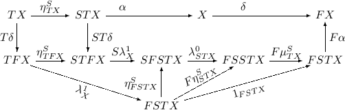
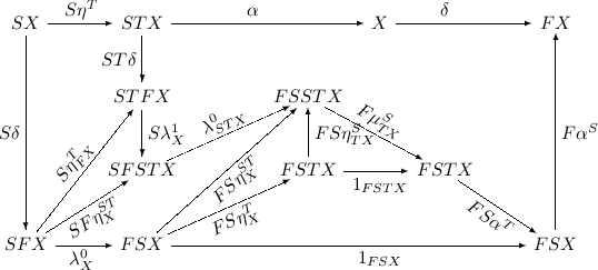
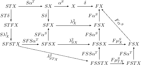
5 The Generalized Powerset Construction for Composite Distributive Laws

We can now formulate a two-step version of the generalized powerset construction, in the setting where we are given three distributive laws $\lambda ^0, \lambda ^1, \lambda ^2$ as in the previous section. Here the extensions can be specified as

$$\begin{aligned} \delta ^\sharp \; = \; F\mu ^{ST}_X \circ \lambda ^1_{STX} \circ T\delta \qquad \text {and} \qquad \hat{\delta } \; = \; F\mu ^S_{TX} \circ \lambda ^2_{STX} \circ S\delta ^\sharp . \end{aligned}$$

giving the following diagram if a final F-coalgebra exists:

We derive the following specification of $\hat{\delta }$ directly in terms of $\delta$:

$$\begin{aligned} \hat{\delta } = F\mu ^S_{TX} \circ \lambda ^2_{STX} \circ SF\mu ^{ST}_X \circ S\lambda ^1_{STX} \circ ST\delta \end{aligned}$$

Proposition 8

The extension $\hat{\delta }$ obtained by the above two step extension coincides with the extension obtained in one step using the distributive law $\hat{\lambda }: (ST)F \Rightarrow F(ST)$. In other words:

$$\begin{aligned} F\mu ^S_{TX} \circ \lambda ^2_{STX} \circ SF\mu ^{ST}_X \circ S\lambda ^1_{STX} \circ ST\delta = F\mu ^{ST}_X \circ \hat{\lambda }_{STX} \circ ST\delta \end{aligned}$$

Proof

The following commuting diagram

establishes that $F\mu ^S_{TX} \circ FS\mu ^{ST}_X = F\mu ^{ST}_X \circ F\mu ^S_{TSTX}$.

Next, observe that

$$\begin{aligned}&F\mu ^S_{TX} \circ \lambda ^2_{STX} \circ SF\mu ^{ST}_X \circ S\lambda ^1_{STX} \circ ST\delta \\ = \;&F\mu ^S_{TX} \circ FS\mu ^{ST}_X \circ \lambda ^2_{STSTX} \circ S\lambda ^1_{STX} \circ ST\delta \quad \text {(naturality) } \\ = \;&F\mu ^{ST}_X \circ F\mu ^S_{TSTX} \circ \lambda ^2_{STSTX} \circ S\lambda ^1_{STX} \circ ST\delta \quad \text {(result of above diagram) }\\ = \;&F\mu ^{ST}_X \circ \hat{\lambda }_{STX} \circ ST\delta \end{aligned}$$

completing the proof.    $\square$

As a result of this proposition, we can directly conclude that, in the two-step diagram above, FSTX can again be assigned the structure of an algebra for the monad ST, and the mappings $\hat{\delta }$ and $\llbracket {-} \rrbracket$ are ST-algebra morphisms.

Finally note that, if F is a cofree copointed functor $(\mathrm {Id} \times G)$, the same considerations as those surrounding the diagrams in (1) again apply.

Remark 9

Note that, when instantiating the above construction with the laws $\lambda ^0$ from Sect. 2.2, $\lambda ^{\text {brz}}$, and $\lambda ^2$ from 2.3, the resulting composite distributive law is a law between the monad ${S} \langle {-} \rangle$ and the cofree copointed endofunctor on $K \times -^A$. This law differs from (but is closely related to) the laws obtained in [WBR13, MPW16], in which a distributive law is defined between a suitably defined monad on ${K} \langle {A + -} \rangle$ and the endofunctor $K \times -^A$ (without copoint). However, the resulting law $\hat{\lambda }$ still has the property, that a language is context-free (resp. a power series is constructively algebraic) iff it is the final coalgebra semantics of the determinization of a finite $K \times {K} \langle {-} \rangle ^A$-coalgebra.

6 Comparison to the Coherence Condition from [Che07]

In [Che07], a similar coherence condition to the one from this paper is presented, providing a way of iterating distributive laws between which a coherence condition similar to (but simpler than) the one presented in this paper is used. We will concentrate on the specific case of just three monads with interacting distributive laws, as the more general iterated cases are less directly relevant to the present paper. In this case, the main result from [Che07] instantiates as:

Proposition 10

Given monads $(S, \eta ^S, \mu ^S)$, $(T, \eta ^T, \mu ^T)$, and $(U, \eta ^U, \mu ^U)$, together with distributive laws $\lambda ^0: UT \Rightarrow TU$, $\lambda ^1: US \Rightarrow SU$, and $\lambda ^2: TS \Rightarrow ST$, if the diagram

(called the coherence condition or Yang-Baxter condition) commutes, the natural transformations

$$\begin{aligned} \lambda ^2 U \circ T\lambda ^1 : (TU)S \Rightarrow S(TU) \end{aligned}$$

and

$$\begin{aligned} S \lambda ^0 \circ \lambda ^1 T : U(ST) \Rightarrow (ST)U \end{aligned}$$

are distributive laws between monads (of the composite monad TU over S, and of U over the composite monad ST), respectively). Moreover both of these laws yield the same composite monad on STU.

A difference between this result and the corresponding result from our paper is that the result in [Che07] is only presented in one direction, instead of as an equivalence. Thus, one can wonder if in this case, too, the result can be turned into an equivalence. In fact, it can be stated in the form of the following three-way equivalence:

Proposition 11

Given monads S, T, and U and distributive laws $\lambda ^0$, $\lambda ^1$, and $\lambda ^2$ as in the previous proposition, the following are equivalent:

• 1. The Yang-Baxter condition holds.

• 2. $\lambda ^2 U \circ T \lambda ^1$ is a distributive law of the composite monad TU over S.

• 3. $S \lambda ^0 \circ \lambda ^1 T$ is a distributive law of U over the composite monad ST.

As a variant on this result, bridging the gap between it and our result, we will move to a setting where, rather than three monads, we have two monads, $(S, \eta ^S, \mu ^S)$ and $(T, \eta ^T, \mu ^T)$ and an endofunctor F, together with a distributive law between monads $\lambda ^0: TS \Rightarrow ST$, and two distributive laws of the monad-over-endofunctor type, $\lambda ^1: TF \Rightarrow FT$, and $\lambda ^2: SF \Rightarrow FS$. We now obtain the following result, in much the same manner as before:

Proposition 12

Given monads $(S, \eta ^S, \mu ^S)$, $(T, \eta ^T, \mu ^T)$, and an endofunctor F, together with distributive laws $\lambda ^0: TS \Rightarrow ST$, $\lambda ^1: TF \Rightarrow FT$, and $\lambda ^2: SF \Rightarrow FS$, the following are equivalent:

• 1. The Yang-Baxter condition holds, as follows:

  

  (3)

• 2. $\lambda ^2 T \circ S \lambda ^1$ is a distributive law of the composite monad ST over F.

(Note that this result is very similar to, but different from, one direction of [BMSZ15, Proposition 7.1], which is concerned with two monads, an endofunctor, and one distributve law between these monads, and two Kleisli-type laws, i.e. laws of the endofunctor over both of the monads.)

In fact, the result can be related to the results from Sect. 4 by means of Lemma 2 and the following proposition:

Proposition 13

Given monads $(S, \eta ^S, \mu ^S)$ and $(T, \eta ^T, \mu ^T)$, an endofunctor F, and distributive laws $\lambda ^0: TS \Rightarrow ST$, $\lambda ^1: TF \Rightarrow FT$, and $\lambda ^2: SF \Rightarrow FS$, the Yang-Baxter condition (3) holds if and only if the law $\hat{\lambda }^1 = F\eta ^ST \circ \lambda ^1 : TF \Rightarrow FST$ makes diagram (2) (Sect. 4) commute.

Connecting this result to the three product rules mentioned in this paper, we recall that the Hadamard product rule can also be given directly as a distributive law of type $TF \Rightarrow FT$ (with $T = -^*$, $F = K \times -^A$) using the strength operator. This law can be given concretely by

$$\begin{aligned} \lambda _X \Bigg ( \prod _{i=1}^n (o_i, a \mapsto d_{ia}) \Bigg ) = \Bigg ( \prod _{i=1}^n o_i, a \mapsto \prod _{k=1}^n d_{ia} \Bigg ) \end{aligned}$$

with the difference that the right hand side is now regarded as an element of FT, instead of an element of FST (with $S = \mathrm {Lin}_{K}({-})$). The Leibniz and Brzozowski product rules, however, do not fit into this simpler scheme, as a direct result of the occurrence of a summation on the right hand side.

It thus turns out that, while the results from [Che07] are easily modified to a coalgebraic setting with laws $\lambda ^0: TS \Rightarrow ST$, $\lambda ^1: TF \Rightarrow FT$, and $\lambda ^2: SF \Rightarrow FS$, the usage of distributive laws into a composite monad (where $\lambda ^1$ is of the form $TF \Rightarrow FST$) allows us to specify product rules of the type $(xy)_a = x_y a + o(x)y_a$, where a summation occurs in the right hand side, that are not possible to specify in a two-step mechanism using the simple variant of the result in [Che07].

Additionally, in the case of distributive laws into composite monads, we require an octagonal coherence condition, rather than the hexagonal condition from [Che07].

7 Further Directions

One interesting direction for future work consists of making a further generalization from copointed functors to comonads. Another possible direction, owing inspiration to [Wor09] (where it is shown that K-algebras are precisely the monoids in the monoidal category of K-semimodules), consists of investigating whether we can reverse the order of the two-step process in the concrete setting of product rules, going from X via $\mathrm {Lin}_{K}({X})$ to ${K} \langle {X} \rangle$ instead of via $X^*$. Finally, it may be very worthwhile to further develop the Prolog-program, developed here in an ad hoc manner to prove a part of Theorem 5, into a more general tool able to (at least in certain contexts) prove commutativity of diagrams.

References

Awodey, S.: Category Theory. Oxford University Press, Oxford (2010)
Bartels, F.: On generalized coinduction and probabilistic specification formats. Ph.D. thesis, Vrije Universiteit Amsterdam (2004)
Bonchi, F., Bonsangue, M.M., Boreale, M., Rutten, J., Silva, A.: A coalgebraic perspective on linear weighted automata. Inf. Comput. 211, 77–105 (2012)
Beck, J.: Distributive laws. In: Eckmann, B. (ed.) Seminar on Triples and Categorical Homology Theory, pp. 119–140. Springer, Heidelberg (1969)
Bonsangue, M.M., Hansen, H.H., Kurz, A., Rot, J.: Presenting distributive laws. In: Heckel, R., Milius, S. (eds.) CALCO 2013. LNCS, vol. 8089, pp. 95–109. Springer, Heidelberg (2013)
Bonchi, F., Milius, S., Silva, A., Zanasi, F.: Killing epsilons with a dagger: a coalgebraic study of systems with algebraic label structure. Theoret. Comput. Sci. 604, 102–126 (2015). doi:10.1016/j.tcs.2015.03.024
Bonsangue, M.M., Rutten, J., Winter, J.: Defining context-free power series coalgebraically. In: Pattinson and Schröder [PS12], pp. 20–39
Brzozowski, J.A.: Derivatives of regular expressions. J. ACM 11, 481–494 (1964)
Barr, M., Wells, C.: Toposes, Triples, and Theories. Grundlehren der mathematischen Wissenschaften. Springer, New York (1985)
Cheng, E.: Iterated distributive laws (2007). http://arxiv.org/pdf/0710.1120v1.pdf
Eilenberg, S.: Automata, Languages, and Machines. Academic Press Inc., Orlando (1976)
Jacobs, B.: A bialgebraic review of deterministic automata, regular expressions and languages. In: Futatsugi, K., Jouannaud, J.-P., Meseguer, J. (eds.) Algebra, Meaning, and Computation. LNCS, vol. 4060, pp. 375–404. Springer, Heidelberg (2006)
Jacobs, B.: Distributive laws for the coinductive solution of recursive equations. Inf. Comput. 204(4), 561–587 (2006)
Jacobs, B., Silva, A., Sokolova, A.: Trace semantics via determinization. In: Pattinson and Schröder [PS12], pp. 109–129
Klin, B.: Bialgebras for structural operational semantics: an introduction. Theoret. Comput. Sci. 412(38), 5043–5069 (2011)
Lenisa, M., Power, J., Watanabe, H.: Distributivity for endofunctors, pointed and co-pointed endofunctors, monads and comonads. Electr. Notes Theor. Comput. Sci. 33, 230–260 (2000)
MacLane, S.: Categories for the Working Mathematician. Springer, New York (1971)
Milius, S., Moss, L.S., Schwencke, D.: Abstract GSOS rules and a modular treatment of recursive definitions. Logical Methods Comput. Sci. 9(3) (2013)
Milius, S., Pattinson, D., Wißmann, T.: A new foundation for finitary corecursion. CoRR, abs/1601.01532 (2016)
Pattinson, D., Schröder, L. (eds.): CMCS 2012. LNCS, vol. 7399. Springer, Heidelberg (2012)
Rosenkranz, M., Regensburger, G.: Integro-differential polynomials and operators. In: Proceedings of the Twenty-First International Symposium on Symbolic and Algebraic Computation, ISSAC 2008, pp. 261–268. ACM, New York (2008)
Rutten, J.J.M.M.: Automata and coinduction (an exercise in coalgebra). In: Sangiorgi, D., de Simone, R. (eds.) CONCUR 1998. LNCS, vol. 1466, pp. 194–218. Springer, Heidelberg (1998)
Rutten, J.: Universal coalgebra: a theory of systems. Theoret. Comput. Sci. 249(1), 3–80 (2000)
Rutten, J.: Behavioural differential equations: a coinductive calculus of streams, automata, and power series. Theoret. Comput. Sci. 308(1–3), 1–53 (2003)
Rutten, J.: A coinductive calculus of streams. Math. Struct. Comput. Sci. 15(1), 93–147 (2005)
Silva, A., Bonchi, F., Bonsangue, M.M., Rutten, J.: Generalizing the powerset construction, coalgebraically. In: Lodaya, K., Mahajan, M. (eds.) FSTTCS. LIPIcs, vol. 8, pp. 272–283. Schloss Dagstuhl–Leibniz-Zentrum für Informatik (2010)
Silva, A., Bonchi, F., Bonsangue, M., Rutten, J.: Generalizing determinization from automata to coalgebras. Logical Methods Comput. Sci. 9(1) (2013)
Schwencke, D.: Compositional and effectful recursive specification formats. Ph.D. thesis, Technische Universität Braunschweig (2014)
Winter, J., Bonsangue, M.M., Rutten, J.: Context-free languages, coalgebraically. In: Corradini, A., Klin, B., Cîrstea, C. (eds.) CALCO 2011. LNCS, vol. 6859, pp. 359–376. Springer, Heidelberg (2011)
Winter, J., Bonsangue, M.M., Rutten, Jan J. M. M : Coalgebraic characterizations of context-free languages. Logical Methods Comput. Sci. 9(3:14) (2013)
Winter, J.: Coalgebraic characterizations of automata-theoretic classes. Ph.D. thesis, Radboud Universiteit Nijmegen (2014)
Worthington, J.: Automata, representations, and proofs. Ph.D. thesis, Cornell University (2009)
Acknowledgements
For various discussions, comments, and criticism (hopefully in all cases taken as constructively as possible), I would like to thank Henning Basold, Marcello Bonsangue, Helle Hvid Hansen, Bart Jacobs, Bartek Klin, Jurriaan Rot, Jan Rutten, and Alexandra Silva, as well as to Charles Paperman for suggesting automation of the proofs (which in the end was carried out for only a part of just one of the propositions). Additionally I would like to thank the anonymous referees (as well as the anonymous refees of the earlier, rejected, submission) for a large amount of corrections and constructive comments.
Author information
Authors and Affiliations
Corresponding author
Editor information
Editors and Affiliations
Rights and permissions
Copyright information
© 2016 IFIP International Federation for Information Processing
About this paper
Cite this paper
Winter, J. (2016). Product Rules and Distributive Laws. In: Hasuo, I. (eds) Coalgebraic Methods in Computer Science. CMCS 2016. Lecture Notes in Computer Science(), vol 9608. Springer, Cham. https://doi.org/10.1007/978-3-319-40370-0_8
Download citation
DOI: https://doi.org/10.1007/978-3-319-40370-0_8
Published:
Publisher Name: Springer, Cham
Print ISBN: 978-3-319-40369-4
Online ISBN: 978-3-319-40370-0
eBook Packages: Computer ScienceComputer Science (R0)