Affine Monads and Side-Effect-Freeness

Abstract

The notions of side-effect-freeness and commutativity are typical for probabilistic models, as subclass of quantum models. This paper connects these notions to properties in the theory of monads. A new property of a monad (‘strongly affine’) is introduced. It is shown that for such strongly affine monads predicates are in bijective correspondence with side-effect-free instruments. Also it is shown that these instruments are commutative, in a suitable sense, for monads which are commutative (monoidal).

B. Jacobs—The research leading to these results has received funding from the European Research Council under the European Union’s Seventh Framework Programme (FP7/2007-2013)/ERC grant agreement nr. 320571.

1 Introduction

In a recent line of work in categorical quantum foundations [3–6, 13, 16] the notion of effectus has been proposed. Within that context one associates an instrument with each predicate, which performs measurement. These instruments are coalgebras, of a particular form, which may change the state. Indeed, it is one of the key features of the quantum world that measurement can change the object under observation. Thus, observation may have a side-effect.

In [6] a subclass of commutative effectuses is defined where there is a one-to-one correspondence between predicates and side-effect-free instruments. These commutative effectuses capture the probabilistic models, as special case of quantum models. Examples of commutative effectuses are the Kleisli categories $\mathcal {K}{}\ell (\mathcal {D})$ and $\mathcal {K}{}\ell (\mathcal {G})$ of the distribution monad $\mathcal {D}$ and the Giry monad $\mathcal {G}$, and the category of commutative von Neumann algebras.

The starting point for the work presented here is: can we translate these notions of side-effect-freeness and commutativity from effectus theory to the theory of monads — and coalgebras of monads — since they are instrumental in the semantics of programming languages? Especially, is there a connection between:

• 1. side-effect-freeness of measurment-instruments and the property that a monad is affine (that is, preserves the final object);

• 2. commutativity as in effectus theory and commutativity of a monad?

The main point of the paper is that these questions can be answered positively.

The first question makes sense because both the distribution and the Giry monad are affine, and it seems that this property is typical for monads that are relevant in probability theory. We shall see below that we actually need a slightly stronger property than ‘affine’, namely what we call ‘strongly affine’.

Given the terminological coincidence, the second question may seem natural, but the settings are quite different and a priori unrelated. Here we do establish a connection, via a non-trivial calculation.

The relation between predicates and associated actions (instruments / coalgebras) comes from quantum theory in general, and effectus theory in particular. This relationship is complicated in the quantum case, but quite simple in the probabilistic case (see Theorem 1 below). It is the basis for a novel logic and type theory for probabilism in [4] (see also [17]).

The background of this work is effectus theory [6] in which logic (in terms of effect modules) and instruments play an important role. Here we concentrate on these instruments, and show that they can be studied in the theory of monads, independent of the logic of effect modules. Including these effect modules in the theory (for special monads) is left to future work.

2 Preliminaries

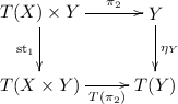
We assume that the reader is familiar with the notion of monad. We recall that a monad $T = (T, \eta , \mu )$ on a category with finite products $(\times , 1)$ is called strong if there is a ‘strength’ natural transformation $\mathrm {st}_{1}$ with components $(\mathrm {st}_{1})_{X,Y} :T(X)\times Y \rightarrow T(X\times Y)$ making the following diagrams commute — in which we omit indices, for convenience.

(1)

(2)

Each monad on the category $\mathbf {Sets}$ of sets and functions is automatically strong, via the definition $\mathrm {st}_{1}(u, y) = T(\lambda x.\,\langle x,y\rangle )(u)$.

Given a strength map $\mathrm {st}_{1}:T(X)\times Y \rightarrow T(X\times Y)$ we define an associated version $\mathrm {st}_{2}$ via swapping:

where $\gamma = \langle \pi _{2}, \pi _{1}\rangle$ is the swap map.

The monad T is called commutative (following [19]) when the order of applying strength in two coordinates does not matter, as expressed by commutation of the following diagram.

(3)

We then write dst: $T(X)\times T(Y) \rightarrow T(X\times Y)$ for ‘double strength’, to indicate the resulting single map, from left to right. Notice that $\mathrm {dst}\mathrel {\circ }\gamma = T(\gamma ) \mathrel {\circ }\mathrm {dst}$.

Below we shall use distributive categories. They have finite products $(\times , 1)$ and coproducts $(+,0)$, where products distribute over coproducts, in the sense that the following maps are isomorphisms.

(4)

Swapping yields an associated distributivity map:

It is an easy exercise to show that $\mathrm {dis}_{1}$ and $\mathrm {dis}_{2}$ interact in the following way.

(5)

The strength and distributivity maps also interact in the obvious way. There are two equivalent versions, with $\mathrm {st}_{1}$ and $\mathrm {dis}_{2}$ and with $\mathrm {st}_{2}$ and $\mathrm {dis}_{1}$. We describe the version that we actually need later on — and leave the verification to the meticulous reader.

(6)

The object $2 = 1+1$ will play a special role below. In a distributive category we have two ‘separation’ isomorphisms written as:

(7)

Explicitly, they are defined as:

These separation maps are natural in X and satisfy for instance:

$$\begin{aligned} \begin{array}{rclcrcl} \nabla \mathrel {\circ }\mathrm {sep}_{1} &{} = &{} \pi _{2} &{} &{} \nabla \mathrel {\circ }\mathrm {sep}_{2} &{} = &{} \pi _{1} \\ (\mathord {!}+\mathord {!}) \mathrel {\circ }\mathrm {sep}_{1} &{} = &{} \pi _{1} &{} &{} (\mathord {!}+\mathord {!}) \mathrel {\circ }\mathrm {sep}_{2} &{} = &{} \pi _{2} \\ {[\kappa _{2}, \kappa _{1}]} \mathrel {\circ }\mathrm {sep}_{1} &{} = &{} \mathrm {sep}_{1} \mathrel {\circ }([\kappa _{2}, \kappa _{1}]\!\times \!\mathrm {id}_{}) &{} &{} [\kappa _{2}, \kappa _{1}] \mathrel {\circ }\mathrm {sep}_{1} &{} = &{} \mathrm {sep}_{2} \mathrel {\circ }(\mathrm {id}_{}\!\times \!{[\kappa _{2}, \kappa _{1}])} \end{array} \end{aligned}$$

(8)

These two maps are related via: $\mathrm {sep}_{1} \mathrel {\circ }\gamma = \mathrm {sep}_{2}$, for $\gamma = \langle \pi _{2}, \pi _{1}\rangle$.

In the special case where $X=2$ we have inverses

It is not hard to see that:

$$\begin{aligned} \begin{array}{rcccl} \mathrm {sep}_{1} \mathrel {\circ }\gamma= & {} \mathrm {sep}_{2}= & {} [\kappa _{1}+\kappa _{1}, \kappa _{2}+\kappa _{2}] \mathrel {\circ }\mathrm {sep}_{1} \end{array} \end{aligned}$$

(9)

The isomorphism can be illustrated as:

3 Affine and Strongly Affine Monads

In this section we recall what it means for a monad to be affine (see [11, 20, 21]), and introduce a slightly stronger notion. We describe basic properties and examples.

Definition 1

Let $\mathbf {C}$ be a category with a monad $T:\mathbf {C} \rightarrow \mathbf {C}$.

• 1. Assuming that $\mathbf {C}$ has a final object 1, one calls T affine if the map $T(1) \rightarrow 1$ is an isomorphism, or simply, if $T(1) \cong 1$.

• 2. Assuming that $\mathbf {C}$ has binary products $\times$ and T is a strong monad, we call T strongly affine if the squares below are pullbacks.

  

  (10)

The notion of an ‘affine monad’ is well-known. What we call ‘strongly affine’ is new. The relationship with ordinary affine monads is quite subtle. Example 2 below show that ‘strongly affine’ is really stronger than ‘affine’. But first we describe some properties and examples.

Lemma 1

Let T be a strong monad on a category $\mathbf {C}$ with finite products $(\times , 1)$.

• 1. The monad T is affine iff the diagrams (10) commute. As a result, a strongly affine monad is affine.

• 2. There is at most one mediating (pullback) map for the diagram (10).

The first point gives an alternative formulation of affiness. An older alternative formulation is: $\langle T(\pi _{1}), T(\pi _{2})\rangle \mathrel {\circ }\mathrm {dst}= \mathrm {id}_{}$, see [20, Theorem 2.1], where $\mathrm {dst}$ is the double strength map from (3), for a commutative monad T.

The second point is useful when we wish to prove that a particular monad is strongly affine: we only need to prove existence of a mediating map, since uniqueness holds in general, see Example 1.

Proof

For the first point, let T be affine. We stretch Diagram (10) as follows.

The square on the left commutes by naturality of strength. For the one on the right we use that T(1) is final, so that $\pi _{2} :T(1)\times Y \rightarrow Y$ is an isomorphism, with inverse $\langle \eta _{1} \mathrel {\circ }\mathord {!}_{Y}, \mathrm {id}_{}\rangle$. Hence:

$$\begin{aligned} \begin{array}{rcl} T(\pi _{2}) \mathrel {\circ }\mathrm {st}_{1} &{} = &{} T(\pi _{2}) \mathrel {\circ }\mathrm {st}_{1} \mathrel {\circ }\langle \eta _{1} \mathrel {\circ }\mathord {!}_{Y}, \mathrm {id}_{}\rangle \mathrel {\circ }\pi _{2} \\ &{} = &{} T(\pi _{2}) \mathrel {\circ }\mathrm {st}_{1} \mathrel {\circ }(\eta _{1}\times \mathrm {id}_{}) \mathrel {\circ }\langle \mathord {!}_{Y}, \mathrm {id}_{}\rangle \mathrel {\circ }\pi _{2} \\ &{} \mathop {=}\limits ^{(2)} &{} T(\pi _{2}) \mathrel {\circ }\eta _{1\times Y} \mathrel {\circ }\langle \mathord {!}_{Y}, \mathrm {id}_{}\rangle \mathrel {\circ }\pi _{2} \\ &{} = &{} \eta _{Y} \mathrel {\circ }\pi _{2} \mathrel {\circ }\langle \mathord {!}_{Y}, \mathrm {id}_{}\rangle \mathrel {\circ }\pi _{2} \\ &{} = &{} \eta _{Y} \mathrel {\circ }\pi _{2}. \end{array} \end{aligned}$$

In the other direction, assume that diagrams (10) commute. We consider the special case $X=Y=1$.

The lower triangle commutes by (1). We need to prove that T(1) is final. It suffices to prove that the composite $\eta _{1} \mathrel {\circ }\mathord {!}:T(1) \rightarrow 1 \rightarrow T(1)$ is the identity. This is obtained from the upper triangle:

$$\begin{aligned} \begin{array}{rcccccl} \eta _{1} \mathrel {\circ }\mathord {!}= & {} \eta _{1} \mathrel {\circ }\pi _{2} \mathrel {\circ }\langle \mathrm {id}_{}, \mathord {!}\rangle= & {} \pi _{1} \mathrel {\circ }\langle \mathrm {id}_{}, \mathord {!}\rangle= & {} \mathrm {id}_{}. \end{array} \end{aligned}$$

For the second point in the lemma we prove uniqueness of mediating maps. Assume we have two maps $f,g :Z \rightarrow T(X)\times Y$ with $\pi _{2} \mathrel {\circ }f = \pi _{2} \mathrel {\circ }g$ and $\mathrm {st}_{1} \mathrel {\circ }f = \mathrm {st}_{1} \mathrel {\circ }g$. We then obtain $\pi _{1} \mathrel {\circ }f = \pi _{1} \mathrel {\circ }g$ from:

Example 1

Three examples of affine monads are the distribution monad $\mathcal {D}$ on $\mathbf {Sets}$ for discrete probability, the Giry monad $\mathcal {G}$ on the category $\mathbf {Meas}$ of measurable spaces, for continuous probability, and the expectation monad $\mathcal {E}$ on $\mathbf {Sets}$. We show that all of them are strongly affine.

(1) The elements of $\mathcal {D}(X)$ are the finite formal convex combinations $\sum _{i}r_{i}|{}x_i{}\rangle$ with elements $x_{i}\in X$ and probabilities $r_{i}\in [0,1]$ satisfying $\sum _{i}r_{i}=1$. We can identify such a convex sum with a function $\varphi :X \rightarrow [0,1]$ whose support $\mathrm {supp}(\varphi ) = \{x\;|\;\varphi (x) \ne 0\}$ is finite and satisfies $\sum _{x}\varphi (x) = 1$. We can thus write $\varphi = \sum _{x}\varphi (x)|{}x{}\rangle$.

We have $\mathcal {D}(1) \cong 1$, since the sole element of $\mathcal {D}(1)$ is the distribution $1|{}\!*\!{}\rangle$, where we write $*$ for the element of the singleton set $1 = \{*\}$.

We show that this monad is also strongly affine. So let in Diagram (10) $\varphi \in \mathcal {D}(X\times Y)$ be a given distribution with $\mathcal {D}(\pi _{2})(\varphi ) = 1|{}z{}\rangle$ for a given element $z\in Y$. Let’s write $\varphi = \sum _{x,y}\varphi (x, y)|{}x,y{}\rangle$, so that $\mathcal {D}(\pi _{2})(\varphi )$ is the marginal distribution:

$$ \begin{array}{rcl} \mathcal {D}(\pi _{2})(\varphi )= & {} {\displaystyle \sum }_{y}\big (\sum _{x}\varphi (x,y)\big )\big |{}y{}\big \rangle . \end{array} $$

If this is the trivial distribution $1|{}z{}\rangle$, then $\varphi (x,y) = 0$ for all x and $y\ne z$. We obtain a new distribution $\psi = \mathcal {D}(\pi _{1})(\varphi ) \in \mathcal {D}(X)$, which takes the simple form $\psi (x) = \varphi (x,z)$. The pair $(\psi ,z) \in \mathcal {D}(X)\times Y$ is the unique element giving us the pullback (10), since:

$$ \begin{array}{rcccccccl} \mathrm {st}_{1}\big (\psi , z\big )= & {} \sum _{x}\psi (x)|{}x,z{}\rangle= & {} \sum _{x}\varphi (x,z)|{}x,z{}\rangle= & {} \sum _{x,y}\varphi (x,y)|{}x,y{}\rangle= & {} \psi . \end{array} $$

(2) Next we consider the Giry monad $\mathcal {G}$ on the category $\mathbf {Meas}$ of measurable spaces. The elements of $\mathcal {G}(X)$ are probability measures $\omega :\Sigma _{X} \rightarrow [0,1]$. The unit $\eta :X \rightarrow \mathcal {G}(X)$ is given by $\eta (x)(M) = 1$ if $x\in M$ and $\eta (x)(M) = 0$ if $x\not \in M$, for each $M\in \Sigma _{X}$. The strength map $\mathrm {st}_{1} :\mathcal {G}(X) \times Y \rightarrow \mathcal {G}(X\times Y)$ is defined as the probability measure $\mathrm {st}_{1}(\omega , y) :\Sigma _{X\times Y} \rightarrow [0,1]$ determined by $M\times N \mapsto \omega (M)\cdot \eta (y)(N)$, see also [10, 12, 22].

So let’s consider the situation (10) for $T = \mathcal {G}$, with a joint probability measure $\omega \in \mathcal {G}(X\times Y)$ and an element $z\in Y$ with

$$\begin{aligned} \begin{array}{rcccl} \mathcal {G}(\pi _{2})(\omega )(N)= & {} \omega (X\times N)= & {} \eta (z)(N), \end{array} \end{aligned}$$

(11)

for all $N\in \Sigma _{Y}$. We prove ‘non-entwinedness’ of $\omega$, that is, $\omega$ is the product of its marginals. Abstractly this means $\omega = \mathrm {dst}\big (\mathcal {G}(\pi _{1})(\omega ), \mathcal {G}(\pi _{2})(\omega )\big )$, and concretely:

$$\begin{aligned} \begin{array}{rcl} \omega (M\times N)= & {} \omega (M\times Y) \cdot \omega (X\times N), \end{array} \end{aligned}$$

(12)

for all $M\in \Sigma _{X}$ and $Y\in \Sigma _{Y}$. We distinguish two cases.

• If $z\not \in N$, then, by monotonicity of the probability measure $\omega$,

  $$\begin{aligned} \begin{array}{rcccccl} \omega (M\times N)\le & {} \omega (X\times N)&\mathop {=}\limits ^{(11)}&\eta (z)(N)= & {} 0. \end{array} \end{aligned}$$

  Hence $\omega (M\times N) = 0$. But also:

  $$ \begin{array}{rcccccl} \omega (M\times Y) \cdot \omega (X\times N)&\mathop {=}\limits ^{(11)}&\omega (M\times Y) \cdot \eta (z)(N)= & {} \omega (M\times Y) \cdot 0= & {} 0. \end{array} $$

• If $z\in N$, then $z\not \in \lnot N$, so that:

  

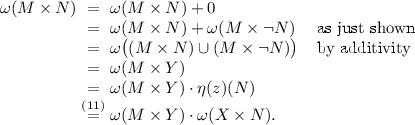
We now take $\phi \in \mathcal {G}(X)$ defined by $\phi (M) = \mathcal {G}(\pi _{1})(\omega )(M) = \omega (M\times Y)$. The pair $(\phi , z) \in \mathcal {G}(X)\times Y$ is then mediating in (10):

$$\begin{aligned} \begin{array}{rcl} \mathrm {st}_{1}(\phi , z)(M\times N) = \phi (M)\cdot \eta (z)(N) &{} = &{} \omega (M\times Y)\cdot \eta (z)(N) \\ &{} \mathop {=}\limits ^{(11)} &{} \omega (M\times Y)\cdot \omega (X\times N) \\ &{} \mathop {=}\limits ^{(12)} &{} \omega (M\times N). \end{array} \end{aligned}$$

Hence the Giry monad $\mathcal {G}$ is strongly affine.

(3) We turn to the expectation monad $\mathcal {E}(X) = \mathbf {EMod} ([0,1]^{X}, [0,1])$ on $\mathbf {Sets}$, where $\mathbf {EMod}$ is the category of effect modules, see [15] for details. Let $h\in \mathcal {E}(X\times Y)$ satisfy $\mathcal {E}(\pi _{2})(h) = \eta (z)$, for some $z\in Y$. This means that for each predicate $q\in [0,1]^{Y}$ we have $h(q \mathrel {\circ }\pi _{2}) = q(z)$.

Our first aim is to prove the analogue of the non-entwinedness equation (12) for $\mathcal {E}$, namely:

$$\begin{aligned} \begin{array}{rcl} h(\mathbf {1}_{U\times V})= & {} h(\mathbf {1}_{U\times Y}) \cdot h(\mathbf {1}_{X\times V}), \end{array} \end{aligned}$$

(13)

for arbitrary subsets $U\subseteq X$ and $V\subseteq Y$. Here we write $\mathbf {1}_{U\times V} :X\times Y \rightarrow [0,1]$ for the obvious indicator function. We distinguish:

• if $z\not \in V$, then $h(\mathbf {1}_{U\times V}) \le h(\mathbf {1}_{X\times V}) = h(\mathbf {1}_{V} \mathrel {\circ }\pi _{2}) = \mathbf {1}_{V}(z) = 0$. Hence (13) holds since both sides are 0.

• if $z\in V$, then $h(\mathbf {1}_{U\times V}) = h(\mathbf {1}_{U\times V}) + h(\mathbf {1}_{U\times \lnot V}) = h(\mathbf {1}_{U\times Y}) = h(\mathbf {1}_{U\times Y}) \cdot h(\mathbf {1}_{X\times V})$.

By [15, Lemma 12] each predicate can be written as limit of step functions. It suffices to prove the result for such step functions, since by [15, Lemma 10] the map of effect modules h is automatically continuous.

Hence we concentrate on an arbitrary step function $p\in [0,1]^{X\times Y}$ of the form $p = \sum _{i,j} r_{i,j} \mathbf {1}_{U_{i}\times V_{j}}$, where the $U_{i} \subseteq X$ and $V_{j}\subseteq Y$ form disjoint covers, and $r_{i,j} \in [0,1]$. We prove that $h(p) = \mathrm {st}_{1}\big (\mathcal {E}(\pi _{1})(h), z\big )(p)$, so that we can take $\mathcal {E}(\pi _{1})(h)\in \mathcal {E}(X)$ to obtain a pullback in (10).

Let $j_0$ be the (unique) index with $z\in V_{j_0}$, so that $p(x,z) = \sum _{i} r_{i,j_0}\mathbf {1}_{U_i}(x)$. Then:

$$\begin{array}{rcl} h(p) = h\big (\sum _{i,j} r_{i,j} \mathbf {1}_{U_{i}\times V_{j}}\big ) &{} = &{} \sum _{i,j}r_{i,j}h\big (\mathbf {1}_{U_{i}\times V_{j}}\big ) \\ &{} \mathop {=}\limits ^{(13)} &{} \sum _{i,j}r_{i,j}h\big (\mathbf {1}_{U_{i}\times Y}\big ) \cdot h\big (\mathbf {1}_{X\times V_{j}}\big ) \\ &{} = &{} \sum _{i,j}r_{i,j}h\big (\mathbf {1}_{U_{i}\times Y}\big ) \cdot \mathbf {1}_{V_{j}}(z) \\ &{} = &{} \sum _{i} r_{i, j_0} h\big (\mathbf {1}_{U_{i}\times Y}\big ) \\ &{} = &{} h\big (\sum _{i} r_{i,j_0} \mathbf {1}_{U_{i}\times Y}\big ) \\ &{} = &{} h\big (\lambda (x,y).\,p(x,z)\big ) \\ &{} = &{} \mathrm {st}_{1}\big (\mathcal {E}(\pi _{1})(h), z\big )(p). \end{array}$$

The following (counter) example is due to Kenta Cho.

Example 2

An example of an affine but not strongly affine monad is the ‘generalised distribution’ monad $\mathcal {D}_{\pm }$ on $\mathbf {Sets}$. Elements of $\mathcal {D}_{\pm }(X)$ are finite formal sums $\sum _i r_i|{}x_i{}\rangle$ with $r_i\in \mathbb {R}$ and $x_i\in X$ satisfying $\sum _i r_i =1$. The other data of a (strong) monad are similar to the ordinary distribution monad $\mathcal {D}$. Clearly $\mathcal {D}_{\pm }(1)\cong 1$, i.e. $\mathcal {D}_{\pm }$ is affine.

Now consider the square (10) with $X=\{x_1,x_2\}$ and $Y=\{y_1,y_2\}$. Define:

$$\begin{array}{rcccl} \varphi= & {} 1|{}x_1,y_1{}\rangle +1|{}x_1,y_2{}\rangle +(-1)|{}x_2,y_2{}\rangle\in & {} \mathcal {D}_{\pm }(X\times Y). \end{array}$$

We have $\mathcal {D}_{\pm }(\pi _2)(\varphi )=1|{}y_1{}\rangle =\eta (y_1)$, since the terms with $y_2$ cancel each other out. But there is no element $\psi \in \mathcal {D}_{\pm }(X)$ such that $\mathrm {st}_{1}(\psi ,y_{1})=\varphi$. Hence the square (10) is not a pullback.

The fact that the terms in this example cancel each other out is known as ‘interference’ in the quantum world. It already happens with negative coefficients. This same monad $\mathcal {D}_{\pm }$ is used in [1]. How the notions of non-locality and contextuality that are studied there relate to strong affineness requires further investigation.

For the record we recall from [2, 23] that each endofunctor on Sets can be written as a coproduct of affine functors.

The following result gives a ‘graph’ construction that is useful in conditional constructions in probability, see the subsequent discussion.

Proposition 1

For a strongly affine monad T there is a canonical bijective correspondence:

What we mean by ‘canonical’ is that the mapping downwards is given by $f \mapsto \mathrm {st}_{1} \mathrel {\circ }\langle f,\mathrm {id}_{}\rangle$.

Proof

The if-part of the statement is obvious, since the correspondence is a reformulation of the pullback property of the diagram (10). In the other direction, let T be strongly affine. As stated, the mapping downwards is given by $\overline{f} = \mathrm {st}_{1} \mathrel {\circ }\langle f,\mathrm {id}_{}\rangle$. Then:

$$\begin{array}{rcccccl} T(\pi _{2}) \mathrel {\circ }\overline{f}= & {} T(\pi _{2}) \mathrel {\circ }\mathrm {st}_{1} \mathrel {\circ }\langle f,\mathrm {id}_{}\rangle&\mathop {=}\limits ^{(10)}&\eta \mathrel {\circ }\pi _{2} \mathrel {\circ }\langle f, \mathrm {id}_{}\rangle= & {} \eta . \end{array}$$

In the other direction we map $g:Y \rightarrow T(X\times Y)$ to $\overline{g} = T(\pi _{1}) \mathrel {\circ }g$. Then:

$$\begin{array}{rcccccl} {\overline{\overline{f}}}= & {} T(\pi _{1}) \mathrel {\circ }\mathrm {st}_{1} \mathrel {\circ }\langle f,\mathrm {id}_{}\rangle&\mathop {=}\limits ^{(1)}&\pi _{1} \mathrel {\circ }\langle f,\mathrm {id}_{}\rangle= & {} f. \end{array}$$

In order to prove $\overline{\overline{g}} = g$ we notice that by the pullback property of diagram (10) we know that there is a unique $h:Y \rightarrow T(X)$ with $g = \mathrm {st}_{1} \mathrel {\circ }\langle h,\mathrm {id}_{}\rangle = \overline{h}$. But then ${\overline{\overline{h}} = h}$, by what we have just shown, so that:

The correspondence in this proposition is used (for the distribution monad $\mathcal {D}$) as Lemma 1 in [9]. There, the map $\mathrm {st}_{1} \mathrel {\circ }\langle f, \mathrm {id}_{}\rangle$ is written as $\mathrm {gr}(f)$, and called the graph of f. It is used in the description of conditional probability. It is also used (implicitly) in [8, §3.1], where a measure/state $\omega \in \mathcal {G}(X)$ and a Kleisli map $f:X \rightarrow \mathcal {G}(Y)$ give rise to a joint probability measure $\mathrm {gr}(f) \mathrel {\bullet }\omega$ in $\mathcal {G}(X\times Y)$.

4 Affine Parts of Monads, and Causal Maps

It is known for a long time that the ‘affine part’ of a monad can be extracted via pullbacks, see [21] (or also [11]). Here we shall relate this affine part to ‘causal’ maps in Kleisli categories of monads.

Proposition 2

Let T be a monad on a category $\mathbf {C}$ with a final object 1. Assume that the following pullbacks exist in $\mathbf {C}$, for each object X.

(14)

Then:

• 1. the mapping $X \mapsto T_{a}(X)$ is a monad on $\mathbf {C}$;

• 2. the mappings $\iota _{X} :T_{a}(X) \rightarrow T(X)$ are monic, and form a map of monads $T_{a} \Rightarrow T$;

• 3. $T_{a}$ is an affine monad, and in fact the universal (greatest) affine submonad of T;

• 4. if T is a strong resp. commutative monad, then so is $T_{a}$.

Proof

These results are standard. We shall illustrate point (3). If we take $X=1$ in Diagram (14), then the bottom arrow $T(\mathord {!}_{X}) :T(X) \rightarrow T(1)$ is the identity. Hence top arrow $T_{a}(1) \rightarrow 1$ is an isomorphism, since isomorphisms are preserved under pullback.

To see that $T_{a} \Rightarrow T$ is universal, let $\sigma :S \Rightarrow T$ be a map of monads, where S is affine, then we obtain a map $\overline{\sigma }_X$ in:

The outer diagram commutes since S is affine, so that $\eta _{1}^{S} \mathrel {\circ }\mathord {!}_{S(1)} = \mathrm {id}_{S(1)}$; then:

Example 3

We list several examples of affine parts of monads.

• 1. Let $\mathcal {M}= \mathcal {M}_{\mathbb {R}_{\ge 0}}$ be the multiset monad on $\mathbf {Sets}$ with the non-negative real numbers $\mathbb {R}_{\ge 0}$ as scalars. Elements of $\mathcal {M}(X)$ are thus finite formal sums $\sum _{i}r_{i}|{}x_i{}\rangle$ with $r_{i}\in \mathbb {R}_{\ge 0}$ and $x_{i}\in X$. The affine part $\mathcal {M}_{a}$ of this monad is the distribution monad $\mathcal {D}$ since $1|{}\!*\!{}\rangle = \mathcal {M}(\mathord {!})(\sum _{i}r_{i}|{}x_i{}\rangle ) = (\sum _{i}r_{i})|{}\!*\!{}\rangle$ iff $\sum _{i}r_{i} = 1$. Thus $\mathcal {D}(X) = \mathcal {M}_{a}(X)$ yields a pullback in Diagram (14).

  The monad $\mathcal {D}_{\pm }$ used in Example 2 can be obtained in a similar manner as an affine part, not of the multiset monad $\mathcal {M}_{\mathbb {R}_{\ge 0}}$ with non-negative coefficients, but from the multiset monad $\mathcal {M}_{\mathbb {R}}$ with arbitrary coefficients: its multisets are formal sums $\sum _{i}r_{i}|{}x_i{}\rangle$ where the $r_i$ are arbitrary real numbers.

• 2. For the powerset monad $\mathcal {P}$ on $\mathbf {Sets}$ the affine submonad $\mathcal {P}_{a} \rightarrowtail \mathcal {P}$ is given by the non-empty powerset monad. Indeed, for a subset $U\subseteq X$ we have:

  $$\begin{array}{rcl} \mathcal {P}(\mathord {!})(U) &{} = &{} \left\{ \begin{array}{ll} \{*\} \quad &{} \text{ if } U \ne \emptyset \\ \emptyset &{} \text{ if } U = \emptyset \end{array}\right. \end{array}$$

  Hence $\mathcal {P}(\mathord {!})(U) = \{*\} = \eta (*)$ iff U is non-empty. It is not hard to see that the non-empty powerset monad $\mathcal {P}_{a}$ is strongly affine.

• 3. Let $T(X) = (S\times X)^{S}$ be the state monad on $\mathbf {Sets}$, for a fixed set of states S. The unit $\eta :X \rightarrow T(X)$ is defined as $\eta (x) = \lambda s\in S.\,(s, x)$ so that the pullback (14) is given by:

  $$\begin{array}{rcl} T_{a}(X) &{} = &{} \{f\in (S\times X)^{S}\;|\;T(\mathord {!})(f) = \eta (*)\} \\ &{} = &{} \{f\in (S\times X)^{S}\;|\;\forall s.\,(\mathrm {id}_{}\times \mathord {!})(f(s)) = (s,*)\} \\ &{} = &{} \{f\in (S\times X)^{S}\;|\;\forall s.\,\pi _{1}f(s) = s\} \\ &{} \cong &{} X^{S}. \end{array}$$

  Thus, Kleisli maps $Y \rightarrow T_{a}(X) = X^{S}$ may use states $s\in S$ to compute the output in X, but they cannot change states: they are side-effect-free.

  In a similar way one shows that the list monad $X \mapsto X^{\star }$ and the lift monad $X \mapsto X+1$ have the identity monad as affine submonad.

• 4. Fix a set C and consider the continuation, (or double-dual) monad $\mathcal {C}$ on $\mathbf {Sets}$ given by $\mathcal {C}(X) = C^{(C^{X})}$, with unit $\eta :X \rightarrow \mathcal {C}(X)$ given by $\eta (x)(f) = f(x)$. The pullback (14) is then:

  $$\begin{array}{rcl} \mathcal {C}_{a}(X) &{} = &{} \{h\in C^{(C^{X})}\;|\;\mathcal {C}(\mathord {!})(h) = \eta (*)\} \\ &{} = &{} \{h\in C^{(C^{X})}\;|\;\forall f\in C^1.\,h(f \mathrel {\circ }\mathord {!}) = f(*)\} \\ &{} = &{} \{h\in C^{(C^{X})}\;|\;\forall c\in C.\,h(\lambda x.\,c) = c\}. \end{array}$$

  This is the submonad of functions $h:C^{X} \rightarrow C$ which have output $c\in C$ on the constant function $\lambda x.\,c :X \rightarrow C$.

We write $\mathcal {K}{}\ell (T)$ for the Kleisli category of a monad T, and we write a fat bullet $\mathrel {\bullet }$ for Kleisli composition $g \mathrel {\bullet }f = \mu \mathrel {\circ }T(g) \mathrel {\circ }f$. For each object X there is a special ‘ground’ map:

This is the result of applying the standard functor $\mathbf {C} \rightarrow \mathcal {K}{}\ell (T)$ to the map $\mathord {!}:X \rightarrow 1$ in the underlying category $\mathbf {C}$.

Causal maps have been introduced in the context of $\mathrm {CP}^*$-categories, see [7], where they express that measurements in the future, given by , cannot influence the past.

Definition 2

A Kleisli map $f:X \rightarrow T(Y)$ will be called causal or unital if it preserves ground, in the sense that:

Causal maps are used in [6] to construct effectuses. Here we define them quite generally, for an arbitrary monad. Notice that each map $f:X \rightarrow T(Y)$ is causal when T is an affine monad. The following elementary observation gives a more precise description.

Lemma 2

A Kleisli map $f:X \rightarrow T(Y)$ is causal if and only if it restricts to a (necessarily unique) map $f':X \rightarrow T_{a}(Y)$ for the affine submonad $\iota :T_{a} \rightarrowtail T$, where $\iota _{Y} \mathrel {\circ }f' = f$.

Proof

Obviously, the causality requirement means that the outer diagram commutes in:

As a result, a Kleisli map $X \rightarrow \mathcal {D}(X)$ for the distribution monad $\mathcal {D}$ can equivalently be described as a causal map $X \rightarrow \mathcal {M}(X)$ for the multiset monad $\mathcal {M}$, see Example 3 (1). This gives a more systematic approach than the “constrained” description from [18], which restricts multisets to a certain subset.

5 Predicates and Instruments

In a very general sense we can define a predicate on an object X in the Kleisli category $\mathcal {K}{}\ell (T)$ of a monad T as a map $p:X \rightarrow 2$, where $2=1+1$, that is as a map $p:X \rightarrow T(2)$ in the underlying category. There is always a ‘truth’ predicate . Similarly there is falsity predicate $\mathbf {0}= \eta \mathrel {\circ }\kappa _{2} \mathrel {\circ }\mathord {!}$, and a negation operation $p^{\bot } = T([\kappa _{2}, \kappa _{1}]) \mathrel {\circ }p$ obtained by swapping. Clearly, $p^{\bot \bot } = p$ and $\mathbf {1}^{\bot } = \mathbf {0}$. In certain cases there is more algebraic structure, see [6], where predicates form effect modules.

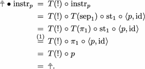
At this stage we informally describe an instrument associated with a predicate $p:X \rightarrow T(1+1)$ as a map $\text {instr}_{p} :X \rightarrow T(X+X)$ with $T(\mathord {!}+\mathord {!}) \mathrel {\circ }\text {instr}_{p} = p$. Such an instrument is called side-effect-free if the following diagram commutes in $\mathcal {K}{}\ell (T)$.

Equivalently, if $T(\nabla ) \mathrel {\circ }\text {instr}_{p} = \eta$ in the underlying category.

This instrument terminology comes from [13] (see also [6]), where it is used in a setting for quantum computation. Here we adapt the terminology to a monad setting. The instrument is used to interpret, for instance, a conditional statement as composite:

For example, for the distribution monad $\mathcal {D}$ a predicate on a set X is a function $p:X \rightarrow \mathcal {D}(1+1) \cong [0,1]$. For such a ‘fuzzy’ predicate there is an instrument map $\text {instr}_{p} :X \rightarrow \mathcal {D}(X+X)$ given by the convex sum:

$$\begin{array}{rcl} \text {instr}_{p}(x)= & {} p(x)|{}\kappa _{1}x{}\rangle + (1-p(x))|{}\kappa _{2}x{}\rangle . \end{array}$$

The associated if-then-else statement gives a weighted combination of the two options, where the weights are determined by the probability $p(x)\in [0,1]$.

Next we describe how such instruments can be obtained via a general construction in distributive categories.

Definition 3

Let T be a strong monad on a distributive category $\mathbf {C}$. For a predicate $p:X \rightarrow T(1+1)$ we define an instrument $\text {instr}_{p} :X \rightarrow T(X+X)$ as composite:

$$\begin{aligned} instr_{p} = \left( {X\mathop \rightarrow \limits ^{{\left\langle {p,id} \right\rangle }} T(2){ \times }X\mathop \rightarrow \limits ^{{{\text {st}}_{1} }} T(2{ \times }X)\mathop \rightarrow \limits _{ \cong }^{{T({\text {sep}}_{1} )}} T(X{ + }X)} \right) \end{aligned}$$

where $\mathrm {sep}_{1}$ is the separation isomorphism from (7).

We collect some basic results about instrument maps.

Lemma 3

In the context of the previous definition we have:

• 1. $T(\mathord {!}+\mathord {!}) \mathrel {\circ }\text {instr}_{p} = p$; in particular, $\text {instr}_{p} = p$ for each $p:1 \rightarrow T(2)$;

• 2. if p is causal, then $\text {instr}_{p}$ is side-effect-free and causal;

• 3. $\text {instr}_{\mathbf {1}} = \eta \mathrel {\circ }\kappa _{1}$ and $\text {instr}_{\mathbf {0}} = \eta \mathrel {\circ }\kappa _{2}$, and $\text {instr}_{p^{\bot }} = T([\kappa _{2}, \kappa _{1}]) \mathrel {\circ }\text {instr}_{p}$;

• 4. for a map $f:Y \rightarrow X$ in the underlying category,

  $$\begin{array}{rcl} T(f+f) \mathrel {\circ }\text {instr}_{p \mathrel {\circ }f}= & {} \text {instr}_{p} \mathrel {\circ }f. \end{array}$$

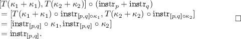
• 5. for predicates $p:X \rightarrow T(2)$ and $q :Y \rightarrow T(2)$,

  $$\begin{array}{rcl} \text {instr}_{[p,q]}= & {} [T(\kappa _{1}+\kappa _{1}), T(\kappa _{2}+\kappa _{2})] \mathrel {\circ }(\text {instr}_{p}+\text {instr}_{q}). \end{array}$$

Proof

We handle these points one by one.

• 1. We have:

  $$\begin{array}{rcl} T(\mathord {!}+\mathord {!}) \mathrel {\circ }\text {instr}_{p} &{} = &{} T(\mathord {!}+\mathord {!}) \mathrel {\circ }T(\mathrm {sep}_{1}) \mathrel {\circ }\mathrm {st}_{1} \mathrel {\circ }\langle p, \mathrm {id}_{}\rangle \\ &{} \mathop {=}\limits ^{(8)} &{} T(\pi _{1}) \mathrel {\circ }\mathrm {st}_{1} \mathrel {\circ }\langle p, \mathrm {id}_{}\rangle \\ &{} \mathop {=}\limits ^{(1)} &{} \pi _{1} \mathrel {\circ }\langle p, \mathrm {id}_{}\rangle \\ &{} = &{} p. \end{array}$$

• 2. Assume that the predicate p is causal, that is . We first show that the instrument $\text {instr}_{p}$ is side-effect-free:

  $$\begin{array}[b]{rcl} T(\nabla ) \mathrel {\circ }\text {instr}_{p} &{} = &{} T(\nabla ) \mathrel {\circ }T(\mathrm {sep}_{1}) \mathrel {\circ }\mathrm {st}_{1} \mathrel {\circ }\langle p, \mathrm {id}_{}\rangle \\ &{} = &{} T(\nabla ) \mathrel {\circ }T(\pi _{2}+\pi _{2}) \mathrel {\circ }T(\mathrm {dis}_{1}^{-1}) \mathrel {\circ }\mathrm {st}_{1} \mathrel {\circ }\langle p, \mathrm {id}_{}\rangle \\ &{} = &{} T(\pi _{2}) \mathrel {\circ }T(\nabla ) \mathrel {\circ }T(\mathrm {dis}_{1}^{-1}) \mathrel {\circ }\mathrm {st}_{1} \mathrel {\circ }\langle p, \mathrm {id}_{}\rangle \\ &{} = &{} T(\pi _{2}) \mathrel {\circ }T(\nabla \times \mathrm {id}_{}) \mathrel {\circ }\mathrm {st}_{1} \mathrel {\circ }\langle p, \mathrm {id}_{}\rangle \\ &{} = &{} T(\pi _{2}) \mathrel {\circ }\mathrm {st}_{1} \mathrel {\circ }(T(\nabla )\times \mathrm {id}_{}) \mathrel {\circ }\langle p, \mathrm {id}_{}\rangle \\ &{} = &{} T(\pi _{2}) \mathrel {\circ }\mathrm {st}_{1} \mathrel {\circ }\langle T(\mathord {!}) \mathrel {\circ }p, \mathrm {id}_{}\rangle \\ &{} = &{} T(\pi _{2}) \mathrel {\circ }\mathrm {st}_{1} \mathrel {\circ }\langle \eta \mathrel {\circ }\mathord {!}, \mathrm {id}_{}\rangle \qquad \text {since}~\textit{p}~\text {is causal} \\ &{} \mathop {=}\limits ^{(2)} &{} T(\pi _{2}) \mathrel {\circ }\eta \mathrel {\circ }\langle \mathord {!}, \mathrm {id}_{}\rangle \\ &{} = &{} \eta \mathrel {\circ }\pi _{2} \mathrel {\circ }\langle \mathord {!}, \mathrm {id}_{}\rangle \\ &{} = &{} \eta . \end{array}$$

  The instrument $\text {instr}_p$ is causal too:

  

• 3. For the truth predicate $\mathbf {1}= \eta \mathrel {\circ }\kappa _{1} \mathrel {\circ }\mathord {!}$ we have:

  $$\begin{array}{rcl} \text {instr}_{\mathbf {1}} &{} = &{} T(\mathrm {sep}_{1}) \mathrel {\circ }\mathrm {st}_{1} \mathrel {\circ }\langle \eta \mathrel {\circ }\kappa _{1} \mathrel {\circ }\mathord {!}, \mathrm {id}_{}\rangle \\ &{} \mathop {=}\limits ^{(2)} &{} T(\mathrm {sep}_{1}) \mathrel {\circ }\eta \mathrel {\circ }\langle \kappa _{1} \mathrel {\circ }\mathord {!}, \mathrm {id}_{}\rangle \\ &{} = &{} \eta \mathrel {\circ }\mathrm {sep}_{1} \mathrel {\circ }\langle \kappa _{1} \mathrel {\circ }\mathord {!}, \mathrm {id}_{}\rangle \\ &{} = &{} \eta \mathrel {\circ }\kappa _{1}. \end{array}$$

  Similarly one obtains $\text {instr}_{\mathbf {0}} = \eta \mathrel {\circ }\kappa _{2}$. Next,

  $$\begin{aligned}&T([\kappa _{2}, \kappa _{1}]) \mathrel {\circ }\text {instr}_{p} \\&= T([\kappa _{2}, \kappa _{1}]) \mathrel {\circ }T(\mathrm {sep}_{1}) \mathrel {\circ }\mathrm {st}_{1} \mathrel {\circ }\langle p, \mathrm {id}_{}\rangle \\&\mathop {=}\limits ^{(8)} T(\mathrm {sep}_{1}) \mathrel {\circ }T([\kappa _{2}, \kappa _{1}]\times \mathrm {id}_{}) \mathrel {\circ }\mathrm {st}_{1} \mathrel {\circ }\langle p, \mathrm {id}_{}\rangle \\&= T(\mathrm {sep}_{1}) \mathrel {\circ }\mathrm {st}_{1} \mathrel {\circ }(T([\kappa _{2}, \kappa _{1}])\times \mathrm {id}_{}) \mathrel {\circ }\langle p, \mathrm {id}_{}\rangle \\&= T(\mathrm {sep}_{1}) \mathrel {\circ }\mathrm {st}_{1} \mathrel {\circ }\langle p^{\bot }, \mathrm {id}_{}\rangle \\&= \text {instr}_{p^\bot }. \end{aligned}$$

• 4. In a straightforward manner we obtain for a map f in the underlying category:

  $$\begin{aligned}&T(f+f) \mathrel {\circ }\text {instr}_{p\mathrel {\circ }f} \\&= T(f+f) \mathrel {\circ }T(\mathrm {sep}_{1}) \mathrel {\circ }\mathrm {st}_{1} \mathrel {\circ }\langle p \mathrel {\circ }f, \mathrm {id}_{}\rangle \\&= T(\mathrm {sep}_{1}) \mathrel {\circ }T(\mathrm {id}_{}\times f) \mathrel {\circ }\mathrm {st}_{1} \mathrel {\circ }\langle p \mathrel {\circ }f, \mathrm {id}_{}\rangle \qquad \text{ by } \text{ naturality } \text{ of } \mathrm {sep}_1 \\&= T(\mathrm {sep}_{1}) \mathrel {\circ }\mathrm {st}_{1} \mathrel {\circ }(\mathrm {id}_{}\times f) \mathrel {\circ }\langle p \mathrel {\circ }f, \mathrm {id}_{}\rangle \\&= T(\mathrm {sep}_{1}) \mathrel {\circ }\mathrm {st}_{1} \mathrel {\circ }\langle p, \mathrm {id}_{}\rangle \mathrel {\circ }f \\&=\text {instr}_{p} \mathrel {\circ }f. \end{aligned}$$

• 5. Via point (4) we get:

  

The main result of this section gives, for strongly affine monads, a bijective correspondence between predicates and side-effect-free instruments.

Theorem 1

Let T be a strongly affine monad on a distributive category. Then there is a bijective correspondence between:

Proof

The mapping downwards is $p \mapsto \text {instr}_{p}$, and upwards is $f \mapsto T(\mathord {!}+\mathord {!}) \mathrel {\circ }f$. Point (2) in Lemma 3 says that $T(\nabla ) \mathrel {\circ }\text {instr}_{p} = \eta$, since p is causal (because T is affine); point (1) tells that going down-up is the identity. For the up-down part we need to show that $f = \text {instr}_{p}$, for $p = T(\mathord {!}+\mathord {!}) \mathrel {\circ }f$. We use the ‘strongly affine’ pullback (10) to get a predicate q in:

The outer diagram commutes by (8). By construction we have $f = \text {instr}_{q}$, see Definition 3. We thus need to prove that $q = p$. But this follows from Lemma 3 (1):

Example 4

We shall illustrate the situation for the powerset monad $\mathcal {P}$ on the (distributive) category $\mathbf {Sets}$. We write $1+1 = 2 = \{0,1\}$, where we identify the element $0\in 2$ with $\kappa _{2}*$ and $1\in 2$ with $\kappa _{1}*$. Hence $\mathcal {P}(2) = \{\emptyset , \{0\}, \{1\}, \{0,1\}\}$ and $\mathcal {P}_{a}(2) = \{\{0\}, \{1\}, \{0,1\}\}$, where $\mathcal {P}_{a} \rightarrowtail \mathcal {P}$ is the affine submonad of non-empty subsets, see Example 3 (2).

For a predicate $p:X \rightarrow \mathcal {P}(2)$ the associated instrument $\text {instr}_{p} :X \rightarrow \mathcal {P}(X+X)$ is, according to Definition 3, given by:

We thus see:

Hence these instruments are not side-effect-free, in general. But if we restrict ourselves to the (strongly affine) submonad $\mathcal {P}_a$ of non-emptyset subsets, then we do have side-effect-freeness — as shown in general in Lemma 3 (2).

In that case we have a bijective correspondence between maps $f:X \rightarrow \mathcal {P}_{a}(X+X)$ with $\mathcal {P}_{a}(\nabla ) \mathrel {\circ }f = \{-\}$ and predicates $p:X \rightarrow \mathcal {P}_{a}(2)$ — as shown in general in Theorem 1.

6 Commutativity

In this section we assume that T is a strong monad on a distributive category $\mathbf {C}$, so that we can associate an instrument $\text {instr}_{p} :X \rightarrow T(X+X)$ with a predicate $p:X \rightarrow T(2)$, like in Definition 3.

Given such a predicate p we define the assert map $\text {asrt}_{p} :X \rightarrow T(X+1)$ as:

$$\begin{array}{rcccl} \text {asrt}_{p}= & {} T(\mathrm {id}_{}+\mathord {!}) \mathrel {\circ }\text {instr}_{p}= & {} T(\pi _{2}+\pi _{1}) \mathrel {\circ }T(\mathrm {dis}_{1}^{-1}) \mathrel {\circ }\mathrm {st}_{1} \mathrel {\circ }\langle p,\mathrm {id}_{}\rangle . \end{array}$$

These assert maps play an important role to define conditional probabilities (after normalisation), see [4]. Here we illustrate how one can define, via these assert maps, a sequential composition operation — called ‘andthen’ — on predicates $p,q:X \rightarrow T(2)$ as:

$$ \begin{array}{rcll} p \mathrel { \& }q &{} = &{} [q, \kappa _{2}] \mathrel {\bullet }\text {asrt}_{p} &{} \text{ in } \mathcal {K}{}\ell (T) \\ &{} = &{} \mu \mathrel {\circ }T([q, T(\kappa _{2}) \mathrel {\circ }\eta ]) \mathrel {\circ }\text {asrt}_{p} \qquad &{} \text{ in } \mathbf {C}. \end{array}$$

This operation incorporates the side-effect of p, if any. Hence, in principle, this is not a commutative operation.

Example 5

We elaborate the situation described above for the state monad $T(X) = (S\times X)^{S}$ from Example 3 (3). A predicate on X can be identified with a map $p:X \rightarrow (S+S)^{S}$, since:

$$\begin{array}{rcccl} T(2)= & {} \big (S\times 2\big )^{S}\cong & {} \big (S + S\big )^{S}. \end{array}$$

For $x\in X$ and $s\in S$ the value $p(x)(s) \in S+S$ describes the ‘true’ case via the left component, and the ‘false’ case via the right component. Clearly, the predicate can also change the state, and thus have a side-effect.

The associated instrument $\text {instr}_{p} :X \rightarrow (S\times (X+X))^{S} \cong (S\times X + S\times X)^{S}$ is described by:

Similarly, $\text {asrt}_{p} :X \rightarrow (S\times (X+1))^{S} \cong (S\times X + S)^{S}$ is:

Hence for predicates $p,q :X \rightarrow (S+S)^{S}$ we have $p\mathrel { \& }q :X \rightarrow (S+S)^{S}$ described by:

The side-effect $s'$ of p is passed on to q, if p holds. Clearly, $\mathrel { \& }$ is not commutative for the state monad.

The theorem below plays a central role for commutativity of the andthen operation $\mathrel { \& }$. It establishes a connection between commutativity of sequential composition and commutativity of the monad, as described in Diagram (3).

Theorem 2

If T is a commutative monad, then instruments commute: for predicates $p,q:X \rightarrow T(2)$, the following diagram commutes in $\mathcal {K}{}\ell (T)$.

(16)

Proof

The structure of the proof is given by the following diagram in the underlying category.

The sub-diagrams (a) commute by naturality, and sub-diagrams (b) by (6) commutation of (c) is equation (9), and the square in the middle is commutativity of the monad T, see (3). Details are left to the interested reader.    $\square$

Corollary 1

For a commutative monad (on a distributive category), sequential composition $\mathrel { \& }$ is commutative on causal predicates.

Proof

We first note that in $\mathcal {K}{}\ell (T)$ we can write . Hence if p, q are both causal, then:

7 Conclusions

We have translated the notions of side-effect-freeness and commutativity from quantum foundations (in the form of effectus theory) to monad theory, and proven some elementary results. This is only a starting point. Expecially, connections between (strong) affineness and non-locality need to be clarified.

Further, the current work forms the basis for a categorical description (that is in the making) of probability theory using strongly affine monads.

We should point out that the setting of the current work is given by distributive categories, with finite cartesian products, and not tensor products. They form in themselves already a classical setting.

References

Abramsky, S., Brandenburger, A.: The sheaf-theoretic structure of non-locality and contextuality. New J. Phys. 13, 113036 (2011)
Adámek, J., Velebil, J.: Analytic functors and weak pullbacks. Theor. Appl. Categ. 21(11), 191–209 (2008)
Adams, R.: QPEL: quantum program and effect language. In: Coecke, B., Hasuo, I., Panangaden, P. (eds.) Electrical Proceedings in Theoretical Computer Science on Quantum Physics and Logic (QPL) 2014, no. 172, pp. 133–153 (2014)
Adams, R., Jacobs, B.: A type theory for probabilistic and Bayesian reasoning (2015). arXiv.org/abs/1511.09230
Cho, K.: Total and partial computation in categorical quantum foundations. In: Heunen, C., Selinger, P., Vicary, J. (eds.) Electrical Proceedings in Theoretical Computer Science on Quantum Physics and Logic (QPL) 2015, no. 195, pp. 116–135 (2015)
Cho, K., Jacobs, B., Westerbaan, A., Westerbaan, B.: An introduction to effectus theory (2015). arXiv.org/abs/1512.05813
Coecke, B., Heunen, C., Kissinger, A.: Categories of quantum and classical channels. Quantum Inf. Process. 1–31 (2014)
Fong, B.: Causal theories: a categorical perspective on Bayesian networks. Master’s thesis, Univ. of Oxford (2012). arXiv.org/abs/1301.6201
Furber, R., Jacobs, B.: Towards a categorical account of conditional probability. In: Heunen, C., Selinger, P., Vicary, J. (eds.) Electronic Proceedings in Theoretical Computer Science of Quantum Physics and Logic (QPL) 2015, no. 195, pp. 179–195 (2015)
Giry, M.: A categorical approach to probability theory. In: Banaschewski, B. (ed.) Categorical Aspects of Topology and Analysis. Lecture Notes in Mathematics, vol. 915, pp. 68–85. Springer, Berlin (1982)
Jacobs, B.: Semantics of weakening and contraction. Ann. Pure Appl. Logic 69(1), 73–106 (1994)
Jacobs, B.: Measurable spaces and their effect logic. In: Logic in Computer Science. IEEE, Computer Science Press (2013)
Jacobs, B.: New directions in categorical logic, for classical, probabilistic and quantum logic. Logical Methods in Comp. Sci. 11(3), 1–76 (2015)
Jacobs, B.: Effectuses from monads. In: MFPS 2016 (2016, to appear)
Jacobs, B., Mandemaker, J.: The expectation monad in quantum foundations. In: Jacobs, B., Selinger, P., Spitters, B. (eds.) Elecronic Proccedings in Theoretical Computer Science of Quantum Physics and Logic (QPL) 2011, no. 95, pp. 143–182 (2012)
Jacobs, B., Westerbaan, B., Westerbaan, B.: States of convex sets. In: Pitts, A. (ed.) FOSSACS 2015. LNCS, vol. 9034, pp. 87–101. Springer, Heidelberg (2015)
Jacobs, B., Zanasi, F.: A predicate/state transformer semantics for Bayesian learning. In: MFPS 2016 (2016, to appear)
Klin, Bartek: Structural operational semantics for weighted transition systems. In: Palsberg, Jens (ed.) Semantics and Algebraic Specification. LNCS, vol. 5700, pp. 121–139. Springer, Heidelberg (2009)
Kock, A.: Monads on symmetric monoidal closed categories. Arch. Math. XXI, 1–10 (1970)
Kock, A.: Bilinearity and cartesian closed monads. Math. Scand. 29, 161–174 (1971)
Lindner, H.: Affine parts of monads. Arch. Math. XXXIII, 437–443 (1979)
Panangaden, P.: Labelled Markov Processes. Imperial College Press, London (2009)
Trnková, V.: Some properties of set functors. Comment. Math. Univ. Carolinae 10, 323–352 (1969)
Acknowledgements
Thanks are due to Kenta Cho and Fabio Zanasi for helpful discussions on the topic of the paper, and to the anonymous referees for suggesting several improvements.
Author information
Authors and Affiliations
Corresponding author
Editor information
Editors and Affiliations
Rights and permissions
Copyright information
© 2016 IFIP International Federation for Information Processing
About this paper
Cite this paper
Jacobs, B. (2016). Affine Monads and Side-Effect-Freeness. In: Hasuo, I. (eds) Coalgebraic Methods in Computer Science. CMCS 2016. Lecture Notes in Computer Science(), vol 9608. Springer, Cham. https://doi.org/10.1007/978-3-319-40370-0_5
Download citation
DOI: https://doi.org/10.1007/978-3-319-40370-0_5
Published:
Publisher Name: Springer, Cham
Print ISBN: 978-3-319-40369-4
Online ISBN: 978-3-319-40370-0
eBook Packages: Computer ScienceComputer Science (R0)