Bottom Fixed Substructure Analysis, Model Testing and Design for Harsh Environment

Abstract

The aim of this chapter is to study the various hydrodynamic loads important for the design process of offshore wind turbines foundations. A numerical study on weakly non-linear waves was conducted, using the commercial code StarCCM++. Open-source codes OpenFoam and OceanWave3D were used for the simulation of breaking waves. Existing analytical and empirical formulations, and the results and conclusions from the current numerical study are presented.

These keywords were added by machine and not by the authors. This process is experimental and the keywords may be updated as the learning algorithm improves.

1 Introduction

The main objective of this study is load analysis on fixed bottom support structures of offshore wind turbines suitable for shallow waters and transitional depths (up to 60 m). Usually, hydrodynamic loads cause lower impact on the tower deflection than the wind loads, however for some conditions hydrodynamic loads excite the structure more severely. Hydrodynamic loads are subject of the study in this research, with the primary focus on impulse forces from the breaking waves.

Quantitative data collection from model tests in the AQUILO¹ project is used for the study on wave propagation and wave loads in the numerical wave tank, by using commercial code StarCCM++. Furthermore, empirical solutions from the Morison equation (Morison et al. 1950) are compared with experimental data as well. Experiments were conducted on support structures installed in the intermediate water depths (d = 40–60 m).

Collaboration with Deltares/Delft within the framework of WiFi², allowed for an insight into comprehensive experimental data for validation of numerical open-source codes—OpenFoam and OceanWave3D. Experiments were conducted on a monopile structure installed in relatively shallow water (d = 30 m). A series of impulse loadings from breaking waves were observed. It is expected that more comprehensive results will be published after completion of the research. In this chapter, a part of the numerical study is presented.

In short, the purpose of this paper is to present the types of hydrodynamic loads important for the design process of offshore wind turbines foundations, to give a note on existing analytical and empirical formulations and to present results and conclusions from the numerical study.

2 Determination of Design Wave

Regular wave profiles in deep water, or intermediate water depth that is not too steep, follow a sinusoidal shape and are well described by linear wave theory. As wave height increases and water depth decreases the wave crest tends to become more narrow and steep, whereas the wave trough becomes long and flat. This happens as the wave starts to sense the bottom. Nonlinearity of wave increases with increased steepness of the wave. Weakly non-linear, undisturbed waves are in general well understood, and higher order perturbation solutions—such as Stokes 3rd, Stokes 5th, and fully non-linear stream function theories—exist for regular waves.

Figure 13.1 shows regions of recommended wave theories. Near the point of breaking, a wave becomes highly nonlinear, and at the point of breaking releases a high amount of energy; such events can have a significant contribution on the loading of offshore wind turbines.

Fig. 13.1

Recommended wave theories (Source: DNV 2014)

Fig. 13.2

Wave elevation time trace; comparison experiment-theories

Sea states are approximated by wave spectra. The Pierson-Moskowitz (Pierson and Moskowitz 1964) and JONSWAP spectrum are commonly used in practice. Generally, the point of interest is the maximum wave elevation in a 3 h storm duration which may occur once in 50-years. Within that duration, the maximum expected wave height can be estimated as H_max = 1.86H_s (DNV 2014), where H_s is significant wave height.

Marked positions on Fig. 13.1 correspond to representative cases from experiments in the AQUILO and WiFi projects. Figure 13.2 presents comparison between experimentally observed wave elevation just before wave breaking and theoritical estimations.

3 Hydrodynamic Loads

The rotor thrust reaction to wind loads acts on a larger lever arm than loads from the waves. Usually, hydrodynamic loads cause a smaller impact on the tower deflection than wind loads. Wind loads are a dominant source of fatigue loading; however in cases when wind and waves are misaligned, there is no influence of aerodynamic damping, and fatigue from hydrodynamic loads has to be taken into consideration as well.

Typical design drivers for foundations of offshore wind turbines are impact forces from very steep and breaking waves (Fig. 13.3), which can be expected at sites where monopile support structures are usually installed (in up to 30 m water depth).

Fig. 13.3

Breaking wave impact (slam) force

The extreme and fatigue response stresses depend strongly on the dynamic behavior of the wind turbine structure. When harmonics of the wave frequency coincide with the natural frequency of the structure, the resonance of the structure may result in an amplification of the response. The foundations of fixed bottom wind turbines are designed such that the natural frequency of the structure is out of the range of wave spectrum frequencies. However, higher harmonics of wave excitation can excite structures in resonance and thus amplify the total response. In literature, the phenomena of “ringing” and “springing” are associated with higher harmonic excitations from the incident wave (Faltinsen 1993).

4 Analytical and Empirical Formulations

4.1 Morison Equation

The Morison equation (Morison et al. 1950) is by far the most used equation for computing wave loads on slender structures such as jackets and monopiles. The inline force on a slender body is estimated from fluid velocities and accelerations. The Morison equation is a sum of two terms; one being an empirical drag term proportional to the fluid velocity squared, and the other being an inertia term, derived from potential flow theory, proportional to the fluid acceleration. The Morison equation is defined as follows:

$$ F=\raisebox{1ex}{$1$}\!\left/ \!\raisebox{-1ex}{$2$}\right.{C}_d\rho D\left|U\right|U+{C}_m\rho A\left|\dot{U}\right| $$

(13.1)

The empirical force coefficients ${C}_m$ and ${C}_d$ in the Morison’s equation are determined from 2D experiments. In general, the drag and inertia coefficients are functions of the Reynolds number, the Keulegan-Carpenter number, the relative roughness, and the ratio between waves and current. The Morison equation which is based on a stream function wave theory predicts the loadings of weakly non-linear waves with good accuracy.

4.2 Higher Harmonic Forces

An amplification of the structural response can be expected when higher harmonics of non-linear waves coincide with the 1st structural natural frequency. The “Ringing” phenomenon is usually associated with third harmonic excitations from incident waves. The reason why the third harmonic force and “ringing” responses are often associated is that f_tower/3 is close to typical peak frequencies of storm waves (Paulsen 2013). When a “ringing” phenomenon is expected, it has to be considered in the design process of wind turbine foundations (DNV 2014).

A comprehensive literature review and a study on higher harmonic loads can be found in the work of (Paulsen 2013). Paulsen (2013) studied higher harmonic loads numerically and compared the obtained results with third order perturbation theories from Faltinsen (1993) and Malenica and Molin (1995). The study by Paulsen (2013) also compared results with the Morison equation with an additional term proposed by Rainey (1989).

4.3 Impulse (Slam) Forces from Breaking Waves

Plunging wave breakers can excite the structure most violently. For the calculation of the impact forces on slender structures, an additional part in the Morison equation is introduced:

$$ F={F}_{Morison}+{F}_{slam}={F}_{inertia}+{F}_{drag}+{F}_{slam} $$

(13.2)

where ${F}_{slam}$[N] is the slam force, defined as the integration of inline impact force, ${f}_i$[N/m], over the area of the impact (Fig. 13.4):

Fig. 13.4

Breaking wave parameters

$$ {F}_{slam}={\int}_0^{area}{f}_i={\eta}_b{\lambda}^{\prime }*fi $$

(13.3)

$$ {F}_{slam}={\eta}_b\lambda *fi;\;\mathrm{rectangular}\;\mathrm{force}\;\mathrm{distribution} $$

(13.4a)

$$ {F}_{slam}=0.5{\eta}_b\lambda *fi;\;\mathrm{triangular}\;\mathrm{force}\;\mathrm{distribution} $$

(13.4b)

The parameter which indicates how much of the wave crest (${\eta}_b$[m]) is active in the impulse force is defined as the “curling factor” ($\lambda$).

The line impact force is generally defined as:

$$ {f}_i={C}_s(t)\rho R{C_b}^2 $$

(13.5)

where Cs is defined as the “slamming coefficient”.

Studies on impact forces from breaking waves are usually compared with one of the first studies on wave entry problems done by Von Karman (1929) and Wagner (1932). They studied impact forces for a case when an infinitely long falling cylinder hits a calm water surface. The cylinder was approximated as a flat plate. Von Karman (1929) considered the momentum conservation during the impact as:

$$ {f}_i=d\left({m}_hV\right)/dt $$

(13.6)

where ${m}_h=0.5\pi \rho {c}^2$ is the added mass below the flat plate.

Wagner (1932) considered the velocity potential around a flat plate as:

$$ \phi =-V\sqrt{c(t)^2-{x}^2} $$

(13.7)

and by estimating $c(t)=2\sqrt{VtR}$, he solved temporal part of the Bernoulli’s equation. Wagner (1932) also explained the so-called “pile-up” effect, which is the deformation of the water free surface around the plate. Due to this “pile-up effect”, the immersion of the cylinder occurs earlier. As a result, the duration of the impact decreases and the maximum impact force increases. Thus, the force calculated by applying Wagner’s theory is estimated as twice the line force calculated by von Karman’s theory (Table 13.1). Both theories are time independent and present only a maximum line force.

Table 13.1 Overview on wave impact studies

For the calculation of impact forces due to plunging wave breakers on offshore wind turbines, a reference is usually made to the model developed by Wienke and Oumeraci (2005). The theoretical description of their model is based on Wagner’s (1932) 2D-model; to account for the temporal development of the impact they compute the non-linear velocity term in Bernoulli’s equation.

Comprehensive experimental studies have been conducted to study impact forces of breaking waves. High fluctuations and scattering from the point of view of local line forces and local pressures are observed. Table 13.1 gives an overview on wave impact studies.

The nature of impulsive forces is characterized by very short durations, and the resulting structural responses are sensitive to dynamic analysis; hence, both the intensity and the time history of impact (slamming) forces are important design parameters. The total impact duration and the “rising time”, are both important parameters for dynamic structure analysis (Fig. 13.5).

Fig. 13.5

Force signal

5 Numerical Analysis

The Navier–Stokes equations can be solved in combination with volume of fluid (VOF) surface capturing scheme. For an incompressible two phase flow, conservation of mass and momentum in an Eulerian frame of reference, is given by:

$$ \nabla \cdot \mathbf{u}=0 $$

(13.8)

$$ \frac{\partial }{\partial \mathrm{t}}\uprho \mathbf{u}+\uprho \left(\nabla \mathbf{u}\right)\mathbf{u}=-\nabla {\mathrm{p}}^{*}-\left(\mathbf{g}\cdot \mathbf{x}\right)\nabla \uprho +\nabla \uprho \left(\boldsymbol{\upmu} \nabla \mathbf{u}\right) $$

(13.9)

where u = (u, v, w) is the instantaneous velocity in Cartesian coordinates, $\uprho$ is the density, ${\mathrm{p}}^{*}$ is the pressure in excess of the hydrostatic pressure, g is the acceleration due to gravity, x is the Cartesian coordinate vector, $\upmu$ is the dynamic molecular viscosity.

The free surface separating the air and water phase is captured using a VOF surface capturing scheme, which solves the following equation for the water volume fraction ($\alpha$):

$$ \frac{\partial \upalpha}{\partial \mathrm{t}}+\nabla \cdot \mathbf{u}\upalpha +\nabla \cdot {\mathbf{u}}_{\mathrm{r}}\upalpha \left(1-\upalpha \right)=0 $$

(13.10)

In Eq. (13.10), u _r is a relative velocity (Berberović et al. 2009), which helps to retain a sharp interface, and the term $\upalpha \left(1-\upalpha \right)$ vanishes everywhere except at the interface. The marker function is 1 when the computational cell is filled with water, and 0 when it is empty; in the free surface zone, the marker function will have a value in the interval $\upalpha \in \left[0;1\right]$ indicating the volume fraction of water and air respectively. The fluid density and viscosity is assumed continuous and differentiable in the entire domain, and the following linear weighting of the fluid properties is adopted:

$$ \uprho =\upalpha {\uprho}_{\mathrm{w}}+\left(1-\upalpha \right){\uprho}_{\mathrm{a}};\;\upmu =\upalpha {\upmu}_{\mathrm{w}}+\left(1-\upalpha \right){\upmu}_{\mathrm{a}} $$

(13.11)

In Eq. (13.9), the sub-indices $\mathrm{w}$ and $\mathrm{a}$ refer to water and air respectively.

5.1 Star CCM++

Numerical analyses within the framework of the AQUILO project were done by using the commercial CFD package StarCCM++. Sensitivity analyses on the regular wave propagation in the numerical domain were also conducted. The inlet boundary condition in the computations is based on the free surface elevation and the velocity components are calculated according to desired wave, using the corresponding wave theory. Wave theories up to the Stokes 5th order theory are implemented in the StarCCM++ package. Waves examined in the scope of the AQUILO can be described as a weakly non-linear and they are well estimated by the Stokes 5th order regular wave theory (Fig. 13.1). The sensitivity of mesh parameters, time step, discretization method and turbulence model was investigated. It was ensured that the reflections from the boundaries were neutralized. The following conclusions were drawn:

• The domain should be refined in the free surface zone (around 25 cells per wave height and 115 cells per wave length); the aspect ratio should be dx/dz ≤ 4 (Fig. 13.6)

  Fig. 13.6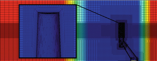

  

  Part of the numerical domain domain, grid refinement

• Second order time discretization should be used with at least five iterations per time step; in the equation for volume fraction of water, the convection flux was discretized using a special high-resolution interface-capturing (HRIC) scheme which is designed to keep the interface sharp. To use the HRIC scheme propagation, the wave should be less than half a cell per time step

• k-ε turbulence models introduce significant generation of eddy viscosity at the free surface interface; significant numerical diffusion was observed. After wave propagation of few wave lengths, wave height was reduced up to the 20 % compared with the initialized wave height.

• Better results were obtained by using an inviscid model. After wave propagation of 20 wave lengths, the wave height was reduced up to the 6 % compared to the initialized wave height

• The structure under analysis must not be placed too close to the inlet boundary because of the reflected waves that propagate upstream toward the inlet boundary and changing inlet values.

• In a case where the linear wave propagating in the numerical tank is influenced by the sea bed, the obtained wave height at the position of interest was around 20 % lower than theoretically expected.

• It was found that the propagation of a wave, influenced by the sea bed, suffers from significant damping. It is suggested that parameters of initialised wave be close to the characteristics of the specific wave of interest.

As waves under the consideration in the AQUILO project are well approximated by Stokes 5th order theory (which is also implemented in the StarCCM++), a “forcing” technique for the further analysis. In the “forcing” technique, the idea is to have free zone around the structure of the interest while, in the rest of the domain, solutions are forced towards theoretical solutions (Fig. 13.7). At each time step, if the solution differs from the theoretical solution it is “forced” towards theoretical solution by assuming an additional source in the transport equation. The additional term in the transport equation is defined as:

Fig. 13.7

“Forcing” technique

$$ {b}_{\phi }=-\lambda \left(\phi -{\phi}^{*}\right) $$

(13.12)

where λ is forcing coefficient; $\phi$ is the solution of the transport equation at the given CV centroid; and ${\phi}^{*}$is the value towards which the solution is forced. This technique is used with very large values of λ, when the solution needs to be fixed to a certain value—after which then the remaining parts of the discretized equation become negligible.

In this technique, waves that are reflected off the structure and propagate upstream towards inlet boundary can be reduced and their influence on results can be eliminated; additionally, the necessary wave damping towards the outlet can be achieved more progressively, and the domain size can be reduced so that the speed of computation is increased.

An almost perfect comparison between the theoretical and numerical computations is presented in Fig. 13.8. As the Stokes 5th order wave theory is the highest wave theory implemented in STAR CCM++, theoretical solutions from other sources need to be employed for an analysis of steeper, strongly non-linear waves.

Fig. 13.8

Comparison between theoretical and computational results

5.2 OceanWave3D: OpenFoam

To correctly predict the nonlinearity of the incident waves, bathymetry changes have to be taken into account as soon as the wave starts to get influenced by the bottom. To simulate the propagation of a wave with a strong influence of the sea bed (very steep, near breaking or breaking waves) the computation domain should be very long—however, the solution would be significantly influenced by numerical diffusion. To reduce the influence of numerical diffusion, and to reduce the time of the computation, one can solve the Navier–Stokes/VOF equations in a very small “inner” region of interest, while wave propagation up to the “inner” region of interest is solved by existing wave theories. A fully non-linear domain decomposed solver is presented by Paulsen et al. (2014). The fully non-linear potential flow solver is combined with a fully non-linear Navier–Stokes/VOF solver via generalized coupling zones of arbitrary shape.

To generate fully nonlinear boundary conditions for the Navier–Stokes/VOF solver, the potential flow solver “OceanWave3D” developed by Engsig-Karup et al. (2009) is applied. The model solves the three dimensional (3D) Laplace problem in Cartesian coordinates while satisfying the dynamic and kinematic boundary conditions. The equations evolve in time using a classic fourth order, five step Runge–Kutta method. The Laplace equation is solved in a $\sigma$-transformed domain using higher order finite differences for numerical efficiency and accuracy. Figure 13.9 depicts a comparison between the irregular wave elevation signal from the OceanWave3D solver, and the same signal measured in the WiFi project for a piston type wave maker.

Fig. 13.9

Comparison of irregular wave elevation, experiment vs. OcenWave3D

The Navier–Stokes/VOF governing equations are solved using an open-source computational fluid dynamics toolbox, OpenFoam®. The equations are discretized using a finite volume approximation with a collocated variable arrangement on generally unstructured grids. For the current investigation, OpenFoam® version 2.3.0 is combined with the open-source wave generation toolbox, waves2Foam.

6 Results

6.1 Stokes 5th Order

Experimental analyses were conducted within the framework of the AQUILO project on four types of support structures: monopile, gravity based, tripod with pile foundation, and gravity tripod structure (Fig. 13.10). Predictions of wave loads are realized with theoretical JONSWAP energy spectra for a potential 50-year storm condition in the Baltic Sea. Global forces and moments on the structures were measured. The geometries do not represent any existing structures, and were designed for purposes of the AQUILO project, by taking into account typical shapes of existing structures and also the feasibility of manufacturing the physical models.

Fig. 13.10

Types of support structures analyzed in the AQUILO project

Due to limitations of the wave maker operability, the depth of the towing tank does not correspond to the design water depths (in a full scale case, the design water depth for a tripod structure is 60 m, while in CTO facilities, the minimum achievable water depth was 120 m). The location of the model relative to the free surface is then adjusted by using an additional support structure mounted to the bottom of the towing tank (Fig. 13.11). Obviously, the difference in water depth results in an incorrect modelling of the wave kinematics. The proposed method of model tests is a necessary compromise resulting from the limitations of the testing facility. In order to minimize the vertical motion of water particles in the vicinity of the foundations, a circular flat plate was mounted below the model (Fig. 13.11).

Fig. 13.11

Installation in the towing tank

As a part of this study, experimental results on tripod gravity structure were compared with results from the Morison equation and numerical computations. Waves which excite the structure with the maximum inline force were taken into the consideration. Drag and inertia coefficients were estimated as Cd = 1.8 and Cm = 2, respectively. The numerical analysis was done with StarCCM++ code, by using the “forcing” technique and an inviscid model. The inviscid model is found to be suitable when the separation of the flow is not expected—i.e.—when the Keulegan-Carpenter number is low (KC < 5) (Faltinsen et al. 1995). A good agreement was observed, as shown in Fig. 13.12.

Fig. 13.12

Comparison of inline force; experiment; Morison; Star CCM++

A local wave breaking was observed during the experimental analysis on the monopile structure equipped with an ice breaking cone (Fig. 13.13). The results of the numerical computation done by StarCCM++ are compared with experimental measurements for the most violent regular wave which can be simulated in the CTO facilities. The comparison results are shown in Fig. 13.14. Because of experimental limitations, the maximum expected wave height could not be simulated (Hmax ≈ 1.86Hs); thus, another numerical simulation was computed on the maximum expected wave height (Fig. 13.15). An impulse peak force caused by the local breaking of wave on the ice breaking cone is clearly visible: the total force increased by approximately 30 % due to the breaking wave.

Fig. 13.13

Monopilestructure equipped with ice-breaking cone; experiment vs Star CCM++

Fig. 13.14

Inline force on monopile equipped with the ice breaking cone; comparison experiment-Star CCM++

Fig. 13.15

Inline force on monopile equipped with the ice breaking cone; Star CCM++

6.2 Breaking Wave

Experimental analyses were conducted within the frame work of the WiFi project on a rigid monopole excited by irregular waves; the waves were estimated using the theoretical JONSWAP energy spectra for an expected 50-year storm condition. A series of impulse forces from breaking waves were observed. The total forces and pressures were measured. Numerical analyses were also conducted by OceanWave3D-OpenFoam interaction, and a good agreement between the measurements and computations was observed (Fig. 13.16).

Fig. 13.16

Comparison of inline force; experiments-OceanWave3D & OpenFoam

The examined waves start breaking just before the front of structure, as shown in Fig. 13.17a, b. The pressure field presented in Fig. 13.17c is relative to the stagnation pressure—which is water density (ρ = 1000 kg/m³) multiplied by the squared wave celerity (c = 2.2 m/s). The maximum computed pressure peak is 1.5ρc². The maximum line force (f_i) is calculated as an integration of the pressure field around the circumference of the cylinder (around 40°) and corresponds to the slamming coefficient value Cs = 1.8. The values of maximum local pressure and slamming coefficient are lower than any values shown in Table 13.1.

Fig. 13.17

Results from numerical analysis; OceanWave3D&OpenFoam

7 Conclusions

A series of computations for hydrodynamic forces on fixed bottom support structures for offshore wind turbines have been carried out. It can be conclusively stated that the Morison equation is an adequate and fast engineering tool for the estimation of inline forces on the slender structures installed in relatively deep water, where strongly non-linear waves are not expected. CFD tools are important for studies related to local flow around the structure, wave run-ups, higher harmonic forces, and impact forces from waves.

It is also noted that simulations of wave propagation (analyses with StarCCM++) suffer from artificial numerical diffusion, especially when k-ε turbulence models are included in the computations. CFD simulations are too expensive and diffusive for simulation of undisturbed wave propagation—which can instead be computed with the potential wave tools, such as OceanWave3D.

An OpenFoam-OceanWave3D interaction was used to simulate breaking waves on a monopile support structure. A very good agreement between measurements and computations was obtained. The maximum obtained peak pressure was 1.5ρc² and the maximum slamming coefficient (Cs) was 1.8, which is quite low compared to the results of studies presented in Table 13.1.

Fig. 13.18

Velocity field under the breaking wave crest

References

Berberović E, van Hinsberg N, Jakirlić S, Roisman I, Tropea C (2009) Drop impact onto a liquid layer of finite thickness: dynamics of the cavity evolution. Phys Rev E 79(3)
Chan ES, Cheong HF, Tan BC (1995) Laboratory study of plunging wave impacts on vertical cylinders. Coast Eng 25:87–107. doi:10.1016/0378-3839(94)00042-V
Chaplin JR (1993) Breaking wave forces on a vertical cylinder. HMSO, London
DNV (2014) Design of offshore wind turbine structures. Offshore Standard DNV-OS-J101
Engsig-Karup AP, Bingham HB, Lindberg O (2009) An efficient flexible-order model for 3D nonlinear water waves. J Comput Phys 228:2100–2118
Fabula AG (1957) Ellipse-fitting approximation of two-dimensional, normal symmetric impact of rigid bodies on water. In: Kuethe AM (ed) Proceedings of the 5th midwestern conference on fluid mechanics, Michigan, April 1957. University of Michigan Press, Michigan, p 299
Faltinsen OM (1993) Sea loads on ships and offshore structures. Cambridge University Press, Cambridge
Faltinsen OM, Newman JN, Vinje T (1995) Nonlinear wave loads on a slender vertical cylinder. J Fluid Mech 289:179–198
Goda Y, Haranaka S, Kitahata M (1966) Study of impulsive breaking wave forces on piles. In: Reports and technical notes. Port and Airport Research Institute (PARI). Available via PARI. http://www.pari.go.jp/search-pdf/vol005-no06.pdf. Accessed 10 Apr 2016
Hildebrandt A, Schlurmann T (2012) Breaking wave kinematics, local pressures, and forces on a tripod support structure. In: Lynett P, Smith JM (eds) 33rd conference on coastal engineering 2012, Santander, July 2012
Malenica Š, Molin B (1995) Third-harmonic wave diffraction by a vertical cylinder. J Fluid Mech 302:203–229
Morison JR, Johnson JW, Schaaf SA (1950) The force exerted by surface waves on piles. J Pet Technol 5:149–154
Paulsen BT (2013) Efficient computations of wave loads on offshore structures. Dissertation, Technical University of Denmark
Paulsen BT, Henrik B, Bingam HB (2014) An efficient domain decomposition strategy for wave loads on surface piercing circular cylinders. Coast Eng 86:57–76
Pierson WJ, Moskowitz L (1964) A proposed spectral form for fully developed wind seas based on the similarity theory of S. A. Kitaigorodskii. J Geophys Res 69(24):5181–5190
Rainey RCT (1989) A new equation for calculating wave loads on offshore structures. J Fluid Mech 204:295–324
Rainey RCT (1995) Slender-body expressions for the wave load on offshore structures. Proc Math Phys Eng Sci 450(1939):391–416
Ros X (2011) Impact forces on a vertical pile from plunging breaking waves. Dissertation, Norwegian University of Science and Technology
Sawaragi T, Nochino M (1984) Impact forces of nearly breaking waves on a vertical circular cylinder. Coast Eng Jpn 27:249–263
Tanimoto K, Takahashi S, Kaneko T et al (1987) Impulsive breaking wave forces on an inclined pile exerted by random waves. In: Edge BL (ed) 20th international conference on coastal engineering, Taipei, November 1986. Coastal Engineering 1986 Proceedings, vol 20. American Society of Civil Engineers, Reston, p 2282
von Karman TH (1929) The impact on seaplane floats during landing. In: National Advisory Committee for Aeronautics (NACA)—Technical Notes NACA-TN-321. Available via NTRS. http://hdl.handle.net/2060/19930081174. Accessed 10 Apr 2016
Wagner H (1932) Über Stoß- und Gleitvorgänge an der Oberfläche von Flüssigkeiten. Z Angew Math Mech 12(4):193–215
Wienke J, Oumeraci H (2005) Breaking wave impact force on a vertical and inclined slender pile-theoretical and large-scale model investigations. Coast Eng 2(5):435–462
Zhou D, Chan ES, Melville WK (1991) Wave impact pressures on vertical cylinders. Appl Ocean Res 13(5):220–234
Acknowledgments
The presented work was realized within the framework of AQUILO project (PBS1/A6/8/2012), co-funded by The National Centre for Research and Development and MareWint project under research area FP7-PEOPLE-2012-ITN Marie-Curie Action : “Initial Training Networks”. Secondment in Deltares was realized under the framework of the joint industry project WiFi (Wave Impacts on Fixed Turbies).
Author information
Authors and Affiliations
Corresponding author
Editor information
Editors and Affiliations
Rights and permissions
Open Access This chapter is distributed under the terms of the Creative Commons Attribution-NonCommercial 4.0 International License (http://creativecommons.org/licenses/by-nc/4.0/), which permits any noncommercial use, duplication, adaptation, distribution and reproduction in any medium or format, as long as you give appropriate credit to the original author(s) and the source, provide a link to the Creative Commons license and indicate if changes were made.
The images or other third party material in this chapter are included in the work’s Creative Commons license, unless indicated otherwise in the credit line; if such material is not included in the work’s Creative Commons license and the respective action is not permitted by statutory regulation, users will need to obtain permission from the license holder to duplicate, adapt or reproduce the material.
Copyright information
© 2016 The Author(s)
About this chapter
Cite this chapter
Veic, D., Kraskowski, M., Bugalski, T. (2016). Bottom Fixed Substructure Analysis, Model Testing and Design for Harsh Environment. In: Ostachowicz, W., McGugan, M., Schröder-Hinrichs, JU., Luczak, M. (eds) MARE-WINT. Springer, Cham. https://doi.org/10.1007/978-3-319-39095-6_13
Download citation
DOI: https://doi.org/10.1007/978-3-319-39095-6_13
Published:
Publisher Name: Springer, Cham
Print ISBN: 978-3-319-39094-9
Online ISBN: 978-3-319-39095-6
eBook Packages: EnergyEnergy (R0)