Alternative Methods to Estimate Implied Variance

Abstract

In this chapter we will introduce how to use Excel to estimate implied volatility. First, we use approximate linear function to derive the volatility implied by Black–Merton–Scholes model. Second, we use nonlinear method, which includes goal seek and bisection method, to calculate implied volatility. Third, we demonstrate how to get the volatility smile using IBM data. Fourth, we introduce constant elasticity volatility (CEV) model and use bisection method to calculate the implied volatility of CEV model. Finally, we calculate the 52 weeks historical volatility of a stock. We used the Excel function webservice to retrieve the 52 historical stock prices.

Appendix 27.1: Application of CEV Model to Forecasting Implied Volatilities for Options on Index Futures

In this appendix, we use CEV model to forecast implied volatility (called IV hereafter) of options on index futures. Cox (1975) and Cox and Ross (1976) developed the “constant elasticity of variance (CEV) model” which incorporates an observed market phenomenon that the underlying asset variance tends to fall as the asset price increases (and vice versa). The advantage of CEV model is that it can describe the interrelationship between stock prices and its volatility. The constant elasticity of variance (CEV) model for a stock price, S, can be represented as follows:

$$ \mathrm{d}\mathrm{S}=\left(\mathrm{r}-\mathrm{q}\right)\mathrm{S}\mathrm{d}\mathrm{t}+{\updelta \mathrm{S}}^{\upalpha}\mathrm{d}\mathrm{Z} $$

(27.1)

where r is the risk-free rate, q is the dividend yield , dZ is a Wiener process, δ is a volatility parameter, and α is a positive constant. The relationship between the instantaneous volatility of the asset return, σ(S, t), and parameters in CEV model can be represented as:

$$ \upsigma \left(\mathrm{S},\mathrm{t}\right)={\updelta \mathrm{S}}^{\upalpha -1} $$

(27.2)

When $\upalpha =1$, the CEV model is the geometric Brownian motion model we have been using up to now. When $\upalpha <1$, the volatility increases as the stock price decreases. This creates a probability distribution similar to that observed for equities with a heavy left tail and a less heavy right tail. When $\upalpha >1$, the volatility increases as the stock price increases, giving a probability distribution with a heavy right tail and a less left tail. This corresponds to a volatility smile where the implied volatility is an increasing function of the strike price. This type of volatility smile is sometimes observed for options on futures.

The formula for pricing a European call option in CEV model is:

$$ {\mathrm{C}}_{\mathrm{t}}=\left\{\begin{array}{l}\hfill {\mathrm{S}}_{\mathrm{t}}{\mathrm{e}}^{-\mathrm{q}\uptau}\left[1-{\upchi}^2\left(\mathrm{a},\ \mathrm{b}+2,\ \mathrm{c}\right)\right]-K{\mathrm{e}}^{-\mathrm{r}\uptau}{\upchi}^2\left(\mathrm{c},\ \mathrm{b},\ \mathrm{a}\right)\kern0.5em when\kern0.5em \alpha <1\hfill \\ {}\hfill {\mathrm{S}}_{\mathrm{t}}{\mathrm{e}}^{-\mathrm{q}\uptau}\left[1-{\upchi}^2\left(\mathrm{c}, - \mathrm{b},\ \mathrm{a}\right)\right]-K{\mathrm{e}}^{-\mathrm{r}\uptau}{\upchi}^2\left(\mathrm{a},\ 2-\mathrm{b},\ \mathrm{c}\right)\kern0.5em when\kern0.5em \alpha >1\hfill \end{array}\right. $$

(27.3)

where $\mathrm{a}=\frac{{\left[{\mathrm{Ke}}^{-\left(\mathrm{r}-\mathrm{q}\right)\uptau}\right]}^{2\left(1-\upalpha \right)}}{{\left(1-\upalpha \right)}^2\upupsilon},\ \mathrm{b}=\frac{1}{1-\upalpha},\ \mathrm{c}=\frac{{{\mathrm{S}}_{\mathrm{t}}}^{2\left(1-\upalpha \right)}}{{\left(1-\upalpha \right)}^2\upupsilon},\kern0.5em \upupsilon =\frac{\updelta^2}{2\left(\mathrm{r}-\mathrm{q}\right)\left(\upalpha -1\right)}\left[{\mathrm{e}}^{2\left(\mathrm{r}-\mathrm{q}\right)\left(\upalpha -1\right)\uptau}-1\right]$ and χ²(z, k, v) is the cumulative probability that a variable with a noncentral χ² distribution¹ with noncentrality parameter v and k degrees of freedom is less than z. Hsu, Lin, and Lee (2008) provided the detailed derivation of approximative formula for CEV model. Based on the approximated formula, CEV model can reduce computational and implementation costs rather than the complex models such as jump-diffusion stochastic volatility model. Therefore, CVE model with one more parameter than Black–Scholes–Merton option pricing model (BSM) can be a better choice to improve the performance of predicting implied volatilities of index options (Singh and Ahmad 2011).

Beckers (1980) investigate the relationship between the stock price and its variance of returns by using an approximative closed-form formulas for CEV model based on two special cases of the constant elasticity class $\left(\alpha =1 or0\right)$. Based on the significant relationship between the stock price and its volatility in the empirical results, Beckers (1980) claimed that CEV model in terms of noncentral chi-square distribution performs better than BC model in terms of log-normal distribution in description of stock price behavior. MacBeth and Merville (1980) is the first paper to empirically test the performance of CEV model. Their empirical results show the negative relationship between stock prices and its volatility of returns; that is, the elasticity class is less than 2 (i.e., $\alpha <2$). Jackwerth and Rubinstein (2001) and Lee et al. (2004) used S&P 500 index options to do empirical work and found that CEV model performed well because it took account the negative correlation between the index level and volatility into model assumption. Pun and Wong (2013) combine asymptotic approach with CEV model to price American options . Larguinho et al. (2013) compute Greek letters under CEV model to measure different dimension to the risk in option positions and investigate leverage effects in option markets.

Since the future price equals the expected future spot price in a risk-neutral measurement, the S&P 500 index futures prices have same distribution property of S&P 500 index prices. Therefore, for a call option on index futures can be given by (27.3) with S_t replaced by F_t and $\mathrm{q}=\mathrm{r}$ as (27.4)²:

$$ {\mathrm{C}}_{\mathrm{t}}^{\mathrm{F}}=\left\{\begin{array}{l}\hfill {\mathrm{e}}^{-\mathrm{r}\uptau}\left({\mathrm{F}}_{\mathrm{t}}\left[1-{\upchi}^2\left(\mathrm{a},\ \mathrm{b}+2,\ \mathrm{c}\right)\right]-K{\upchi}^2\left(\mathrm{c},\ \mathrm{b},\ \mathrm{a}\right)\ \right)\kern1.25em when\kern1em \alpha <1\hfill \\ {}\hfill \hfill \\ {}\hfill {\mathrm{e}}^{-\mathrm{r}\uptau}\left({\mathrm{F}}_{\mathrm{t}}\left[1-{\upchi}^2\left(\mathrm{c}, - \mathrm{b},\ \mathrm{a}\right)\right]-K{\upchi}^2\left(\mathrm{a},\ 2-\mathrm{b},\ \mathrm{c}\right)\right)\kern1em when\kern1em \alpha >1\hfill \end{array}\right. $$

(27.4)

where $\mathrm{a}=\frac{{\mathrm{K}}^{2\left(1-\upalpha \right)}}{{\left(1-\upalpha \right)}^2\upupsilon},\ \mathrm{b}=\frac{1}{1-\upalpha},\ \mathrm{c}=\frac{{{\mathrm{F}}_{\mathrm{t}}}^{2\left(1-\upalpha \right)}}{{\left(1-\upalpha \right)}^2\upupsilon},\kern0.5em \upupsilon ={\updelta}^2\uptau$

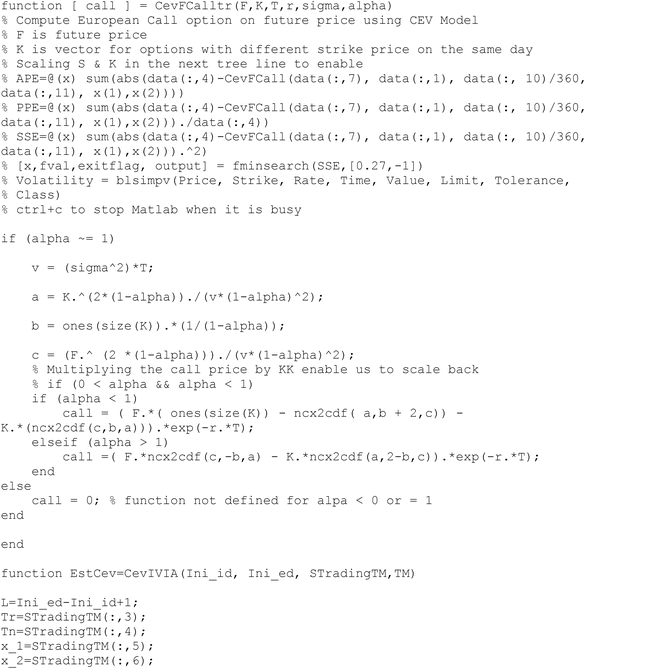
The MATLAB code to price European call option on the future price using CEV model is as follows:

The procedures to obtain estimated parameters of CEV model are as follows:

• 1. Let C ^F_i,n,t be the market price of the nth option contract in category i, $\widehat{{\mathrm{C}}_{\mathrm{i},\mathrm{n},\mathrm{t}}^{\mathrm{F}}}\left({\updelta}_0,{\upalpha}_0\right)$ be the model option price determined by CEV model in (27.4) with the initial value of parameters, $\updelta ={\updelta}_0\ \mathrm{and}\ \upalpha ={\upalpha}_0$. For nth option contract in category i at date t, the difference between market price and model option price can be described as:

  $$ {\upvarepsilon}_{\mathrm{i},\mathrm{n},\mathrm{t}}^{\mathrm{F}}={\mathrm{C}}_{\mathrm{i},\mathrm{n},\mathrm{t}}^{\mathrm{F}}-\widehat{{\mathrm{C}}_{\mathrm{i},\mathrm{n},\mathrm{t}}^{\mathrm{F}}}\left({\updelta}_0,{\upalpha}_0\right) $$

  (27.5)

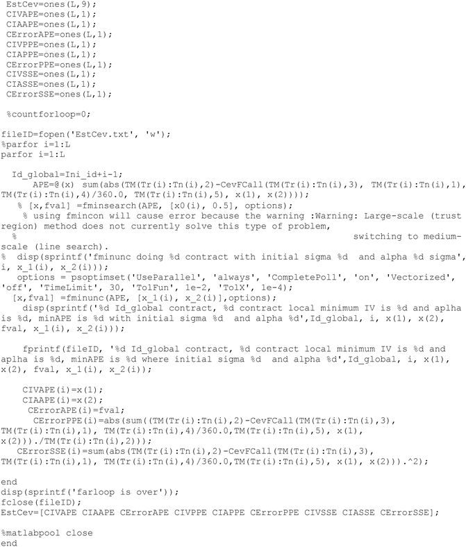
The MATLAB code to find initial value of parameters in CEV model is as follows:

• 2. For each date t, we can obtain the optimal parameters in each group by solving the minimum value of absolute pricing errors (minAPE) as:

  $$ {\mathrm{minAPE}}_{\mathrm{i},\mathrm{t}}=\underset{\updelta_0,{\upalpha}_0}{ \min }{\displaystyle \sum_{\mathrm{n}=1}^{\mathrm{N}}}\left|{\upvarepsilon}_{\mathrm{i},\mathrm{n},\mathrm{t}}^{\mathrm{F}}\right| $$

  (27.6)

  where N is the total number of option contracts in group i at time t.

• 3. Using optimization function in MATLAB to find a minimum value of the unconstrained multivariable function, the function code is as follows:

  $$ \left[\mathrm{x},\ \mathrm{fval}\right]=\mathrm{fminunc}\left({\mathrm{fun},\ \mathrm{x}}_0\right) $$

  (27.7)

  where x is the optimal parameters of CEV model, fval is the local minimum value of minAPE, fun is the specified MATLAB function of (27.4), and x₀ is the initial points of parameters obtained in step (1). The algorithm of fminunc function is based on quasi-Newton method. The MATLAB code is as follows:

  

  

The Data is the options on S&P 500 index futures expired within January 1, 2010, to December 31, 2013, which are traded at the Chicago Mercantile Exchange (CME).³ The reason for using options on S&P 500 index futures instead of S&P 500 index is to eliminate from nonsimultaneous price effects between options and its underlying assets (Harvey and Whaley 1991). The option and future markets are closed at 3:15 pm central time (CT), while stock market is closed at 3 pm CT. Therefore, using closing option prices to estimate the volatility of underlying stock return is problematic even though the correct option pricing model is used. In addition to no nonsynchronous price issue, the underlying assets, S&P 500 inde x futures, do not need to be adjusted for discrete dividends . Therefore, we can reduce the pricing error in accordance with the needless dividend adjustment. According to the suggestions in Harvey and Whaley (1991, 1992a, b), we select simultaneous index option prices and index future prices to do empirical analysis.

The risk-free rate is based on 1-year Treasury Bill from Federal Reserve Bank of St. Louis.⁴ Daily closing price and trading volumes of options on S&P 500 index futures and its underlying asset can be obtained from Datastream.

The future options expired on March, June, and September in both 2010 and 2011 are selected because they have over 1 year trading date (above 252 observations), while other options only have more or less 100 observations. Studying futures option contracts with same expired months in 2010 and 2011 will allow the examination of IV characteristics and movements over time as well as the effects of different market climates.

In order to ensure reliable estimation of IV, we estimate market volatility by using multiple option transactions instead of a single contract. For comparing prediction power of Black model and CEV model, we use all future options expired in 2010 and 2013 to generate implied volatility surface. Here we exclude the data based on the following criteria:

• 1. IV cannot be computed by Black model.

• 2. Trading volume is lower than ten for excluding minuscule transactions.

• 3. Time to maturity is less than 10 days for avoiding liquidity-related biases.

• 4. Quotes not satisfying the arbitrage restriction: excluding option contact if its price larger than the difference between S&P 500 index future and exercise price.

• 5. Deep-in/out-of-money contacts where the ratio of S&P 500 index future price to exercise price is either above 1.2 or below 0.8.

After arranging data based on these criteria, we still have 30,364 observations of future options which are expired within the period of 2010–2013. The period of option prices is from March 19, 2009, to November 5, 2013.

To deal with moneyness- and maturity-related biases, we use the “implied-volatility matrix” to find proper parameters in CEV model. The option contracts are divided into nine categories by moneyness and time to maturity. Option contracts are classified by moneyness level as at-the-money (ATM), out-of-the-money (OTM), or in-the-money (ITM) based on the ratio of underlying asset price, S, to exercise price, K. If an option contract with S/K ratio is between 0.95 and 1.01, it belongs to ATM category. If its S/K ratio is higher (lower) than 1.01 (0.95), the option contract belongs to ITM (OTM) category.

According to the large observations in ATM and OTM, we divide moneyness-level group into five levels: ratio above 1.01, ratio between 0.98 and 1.01, ratio between 0.95 and 0.98, ratio between 0.90 and 0.95, and ratio below 0.90. By expiration day, we classified option contracts into short term (less than 30 trading days), medium term (between 30 and 60 trading days), and long term (more than 60 trading days).

In Fig. 27.1, we find that each option on index future contract’s IV estimated by Black model varies across moneyness and time to maturity. This graph shows volatility skew (or smile) in options on S&P 500 index futures, i.e., the implied volatilities decrease as the strike price increases (the moneyness level decreases).

Fig. 27.1

Implied volatilities in black model

Even though everyday implied volatility surface changes, this characteristic still exists. Therefore, we divided future option contracts into a six by four matrix based on moneyness and time-to-maturity levels when we estimate implied volatilities of future options in CEV model framework in accordance with this character. The whole option samples expired within the period of 2010–2013 contains 30,364 observations. The whole period of option prices is from March 19, 2009, to November 5, 2013. The observations for each group are presented in Table 27.1.

Table 27.1 Average daily and total number of observations in each group

Since most trades are in the future options with short time to maturity, the estimated implied volatility of the option sample s in 2009 may be significantly biased because we didn’t collect the future options expired in 2009. Therefore, we only use option prices in the period between January 1, 2010, and November 5, 2013, to estimate parameters of CEV model. In order to find global optimization instead of local minimum of absolute pricing errors, the range s for searching suitable δ₀ and α₀ are set as ${\updelta}_0\in \left[0.01,0.81\right]$ with interval 0.05 and ${\upalpha}_0\in \left[-0.81,\ 1.39\right]$ with interval 0.1, respectively. First, we find the value of parameters, $\left(\widehat{\updelta_0},\widehat{\alpha_0}\right)$, within the range s such that minimize value of absolute pricing errors in (27.5). Then we use this pair of parameters, $\left(\widehat{\updelta_0},\widehat{\alpha_0}\right)$, as optimal initial estimates in the procedure of estimating local minimum minAPE based on steps (1)–(3). The initial parameter setting of CEV model is presented in Table 27.2.

Table 27.2 Initial parameters of CEV model for estimation procedure

In Table 27.2, the average sigma is almost the same, while the average alpha value in either each group or whole sample is less than one. This evidence implies that the alpha of CEV model can capture the negative relationship between S&P 500 index future prices and its volatilities shown in Fig. 27.1. The instant volatility of S&P 500 index future prices equals to ${\updelta}_0{\mathrm{S}}^{\upalpha_0-1}$ where S is S&P 500 index future prices and δ₀ and α₀ are the parameters in CEV model. The estimated parameters in Table 27.2 are similar across time-to-maturity level but volatile across moneyness.

Because of the implementation and computational costs, we select the subperiod from January 2012 to November 2013 to analyze the performance of CEV model. The total number of observations and the length of trading days in each group are presented in Table 27.3. The estimated parameters in Table 27.2 are similar across time-to-maturity level but volatile across moneyness. Therefore, we investigate the performance of all groups except the groups on the bottom row of Table 27.3. The performance of models can be measured by either the implied volatility graph or the average absolute pricing errors (AveAPE). The implied volatility graph should be flat across different moneyness levels and time to maturity. We use subsample like what Bakshi et al. (1997) and Chen et al. (2009) did to test implied volatility consistency among moneyness-maturity categories. Using the subsample data from January 2012 to May 2013 to test in-the-sample fitness, the average daily implied volatility of both CEV and Black models and average alpha of CEV model are computed in Table 27.4. The fitness performance is shown in Table 27.5. The implied volatility graphs for both models are shown in Fig. 27.2. In Table 27.4, we estimate the optimal parameters of CEV model by using a more efficient program. In this efficient program, we scale the strike price and future price to speed up the program where the implied volatility of CEV model equals to $\updelta \left({\mathrm{ratio}}^{\upalpha -1}\right)$, ratio is the moneyness level, and δ and α are the optimal parameters of program which are not the parameters of CEV model in (27.4). In Table 27.5, we found that CEV model perform well at in-the-money group.

Table 27.3 Total number of observations and trading days in each group

Table 27.4 Average daily parameters of in sample

Table 27.5 AveAPE performance for in-sample fitness

Fig. 27.2

Implied volatilities and CEV alpha graph

Figure 27.2 shows the IV computed by CEV and Black models. Although their implied volatility graphs are similar in each group, the reasons to cause volatility smile are totally different. In Black model, the constant volatility setting is misspecified. The volatility parameter of Black model in Fig. 27.2b varies across moneyless and time-to-maturity levels, while the IV in CEV model is a function of the underlying price and the elasticity of variance (alpha parameter). Therefore, we can image that the prediction power of CEV model will be better than Black model because of the explicit function of IV in CEV model. We can use alpha to measure the sensitivity of relationship between option price and its underlying asset. For example, in Fig. 27.2c, the in-the-money future options near expired date have significantly negative relationship between future price and its volatility.

The better performance of CEV model may result from the over-fitting issue that will hurt the forecastability of CEV model. Therefore, we use out-of-sample data from June 2013 to November 2013 to compare the prediction power of Black and CEV models. We use the estimated parameters in previous day as the current day’s input variables of model. Then, the theoretical option price computed by either Black or CEV model can calculate bias between theoretical price and market price. Thus, we can calculate the average absolute pricing errors (AveAPE) for both models. The lower the value of a model’s AveAPE, the higher the pricing prediction power of the model. The pricing errors of out-of-sample data are presented in Table 27.6. Here we find that CEV model can predict options on S&P 500 index futures more precisely than Black model. Based on the better performance in both in sample and out of sample, we claim that CEV model can describe the options of S&P 500 index futures more precisely than Black model.

Table 27.6 AveAPE performance for out of sample

With regard to generate implied volatility surface to capture whole prediction of the future option market, the CEV model is the better choice than Black model because it not only captures the skewness and kurtosis effects of options on index futures but also has less computational costs than other jump-diffusion stochastic volatility models.

In sum, we show that CEV model performs better than Black model in aspects of either in-sample fitness or out-of-sample prediction . The setting of CEV model is more reasonable to depict the negative relationship between S&P 500 index future price and its volatilities. The elasticity of variance parameter in CEV model captures the level of this characteristic. The stable volatility parameter in CEV model in our empirical results implies that the instantaneous volatility of index future is mainly determined by current future price and the level of elasticity of variance parameter.

References

Bakshi G, Cao C, Chen Z (1997) Empirical performance of alternative option pricing models. J Finance 52:2003–2049
Beckers S (1980) The constant elasticity of variance model and its implications for option pricing. J Finance 35:661–673
Black F, Scholes M (1973) The pricing of options and corporate liabilities. J Polit Econ 81(3):637–654
Chen R, Lee CF, Lee H (2009) Empirical performance of the constant elasticity variance option pricing model. Rev Pacific Basin Financ Markets Policies 12(2):177–217
Corrado CJ, Miller TW (1996) A note on a simple, accurate formula to compute implied standard deviations. J Bank Financ 20:595–603
Cox JC (1975) Notes on option pricing I: constant elasticity of variance diffusions. Working paper, Stanford University
Cox JC, Ross SA (1976) The valuation of options for alternative stochastic processes. J Financ Econ 3:145–166
Harvey CR, Whaley RE (1991) S&P 100 index option volatility. J Finance 46:1551–1561
Harvey CR, Whaley RE (1992a) Market volatility prediction and the efficiency of the S&P 100 index option market. J Financ Econ 31:43–73
Harvey CR, Whaley RE (1992b) Dividends and S&P 100 index option valuation. J Futures Mark 12:123–137
Hsu YL, Lin TI, Lee CF (2008) Constant elasticity of variance (CEV) option pricing model: integration and detailed derivation. Math Comput Simul 79(1):60–71
Jackwerth JC, Rubinstein M (2001) Recovering stochastic processes from option prices. Working paper, London Business School
Larguinho M, Dias JC, Braumann CA (2013) On the computation of option prices and Greeks under the CEV model. Quant Finance 13(6):907–917
Lee CF, Wu T, Chen R (2004) The constant elasticity of variance models: new evidence from S&P 500 index options. Rev Pacific Basin Financ Markets Policies 7(2):173–190
MacBeth JD, Merville LJ (1980) Tests of the Black-Scholes and Cox call option valuation models. J Finance 35:285–301
Merton RC (1973) A rational theory of option pricing. Bell J Econ Manag Sci 4:141–183
Pun CS, Wong HY (2013) CEV asymptotics of American options. J Math Anal Appl 403(2):451–463
Singh VK, Ahmad N (2011) Forecasting performance of constant elasticity of variance model: empirical evidence from India. Int J Appl Econ Financ 5:87–96
Author information
Authors and Affiliations