
Abstract
The histogram-based reversible data hiding scheme (RDH) generated a one-dimensional (1D) histogram distribution. In this article, based on two-dimensional (2D) histogram distribution, a framework of reversible data hiding is proposed by using two side-match predictors, called as Forward side-match (FSM) and Backward side-match (BSM). First, by considering each predicted pixel value, we use two side-match predictors to obtain two prediction error distributions. A slope meter is computed by the differencing of two distributions. Then, a two dimensional histogram is generated by composing of BSM distribution and slope meter. Based on the 2D, more specified spaces can be found to enhance the performance. The experimental results demonstrated that our proposed scheme can achieve better performance in terms of both marked image quality and embedding capacity than that of conventional works.
You have full access to this open access chapter, Download conference paper PDF
Keywords
1 Introduction
Data hiding is an advanced technology for protecting the message with integrity and security from data transmission in a public network [1]. The secret information is capable of being hidden into some media, such as an image, audio or video data, using the well-known data hiding scheme. In general, for different target, the data hiding scheme can be classified into two categories. One is non-reversible data hiding scheme [2–4]. The non-reversible data hiding scheme aims to protect the hidden data for secret communication. The conventional LSBs (least signification bit substitution) is a simple and easy technology of non-reversible data hiding scheme. For example of 1-bit LSBs method, a secret bit is to be embedded into 1-rightmost bit of the cover pixel. The other is reversible data hiding (RDH) scheme [5–16]. The goal of RDH algorithm is to obtain both cover media and hidden data that can be recovered and extracted from stego media. It indicates that the distortion of cover media is intolerable when secret message is extracted. RDH can be widely applied into some applications, such as military, medical, or legal document.
Many RDH techniques have been developed in present. It can be divided into three categories, namely, histogram-based [5–8], difference expansion [9–12], and prediction error [13–16]. Ni et al. first proposed a reversible data hiding based on histogram shifting in 2006 [5]. In their method, the histogram distribution is fist generated from an input image. After that, shift and conceal the secret bits into the selected range from histogram distribution. Ni’s approach performed a good quality in the stego image because pixel shifting and data concealing are only shifted by one unit. Although histogram-based approach is simplicity and provides high image quality, the number of embedding capacity is limited in the height of peak point. Later on, more efficient algorithms have been invented for improving the embedding capacity limitation [6–8].
The second category is difference expansion. In 2003, Tian proposed a reversible data hiding scheme based difference expansion (DE) [9]. Tain’s method expands the two pixel differencing for data concealing. The maximal embedding ratio based on DE is near to 0.5 bpp (bit per pixel) for one layer embedding. Some researchers are focused on investigation and developing high-fidelity reversible data hiding scheme [10–12].
The histogram-based approach and difference expansion method can perform lossless data hiding, but their performance might be limited within the media context. A basic idea is to review their drawback and develop suitable strategy for promoting the performance in terms of embedding capacity and image quality. The prediction error is a good strategy for both histogram-based approach and difference expansion method to devise a new method of improving the performance. A local prediction reversible data hiding combined prediction error and difference expansion is proposed by Drago and Coltur in 2014 [13]. Drago and Colutr’s approach utilized least square predictor to obtain the prediction error, then, expend the prediction error for data hiding. This approach has better performance than that of DE method. Later on, more researchers are developed the efficient approaches for obtaining higher performance [14–16].
In reviewing above-mention reversible data hiding scheme, a framework of reversible data hiding is proposed. Our main contribution is to build 2D histogram distribution based on two side-match predictors and slope meter. 2D histogram distribution can collect more information and find out more spaces for date embedding, resulting in high embedding capacity. Our proposed can be extended into multi-dimensional framework in future.
The rest of the paper is organized as follows. The related works about histogram shifting scheme are briefly introduced in Sect. 2. Section 3 presents our proposed scheme in detail. The experimental result is illustrated in Sect. 4. Finally, the conclusion is concludes in Sect. 5.
2 Related Works
In this subsection, we will review the reversible data hiding scheme based on histogram shifting. The histogram shifting scheme, named as histogram-based, is introduced in 2006. Ni et al.’s approach found out that each cover image has its pixel distribution. Firstly, they applied the statistic function to account each pixel number, the histogram distribution is thus generated. Next, find out the range of peak point and zero point from this distribution. In the end, shift and conceal the data into the range of peak point and zero point. The detail algorithm of histogram-based is shown as below.
Input: Cover image CI, each pixel value x∈[0.255], secret message SM = b 1 b 2 b 3 …b n , b i ∈ {0,1}.
Output: Stego image SI, a pair information (peak point, zero point).
-
Step 1:
Generate a histogram distribution H(x) from an inputted image. Where, Fig. 1 is an example of histogram distribution using Lena image.
Fig. 1. 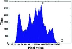
The example of pixel distribution using Lena as cover image
-
Step 2:
Find out a pair-data (P, Z) from the histogram distribution. Notable, P indicates the maximum number of pixels in this distribution. Z means no pixel or minimum pixel in this distribution.
-
Step 3:
Shift all the pixels x within the range of peak point and zero point by one unit. Note, the Fig. 2 shows the result after pixel shifting operation. The shifting function is given as following.
$$ \left\{ {\begin{array}{*{20}c} {x^{\prime} = x + 1,\text{if }Z > P\;\text{and}\;x \in \left[ {\text{P + 1, Z}} \right]} \\ {x^{\prime} = x - 1,\text{if }P > Z\;\text{and}\;x \in \left[ {\text{Z, P} - \text{1}} \right]} \\ \end{array} } \right. $$(1)Fig. 2. 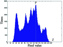
The example of pixel shifting using Fig. 1.
-
Step 4:
Scan all pixels in the cover image, once the pixel value meets the P value, and then, check the secret bits. If the secret bit is “0”, the pixel value remains unchanged. If the secret bit is “1”, the pixels value is changed by one unit according to following data concealing function
$$ \left\{ {\begin{array}{*{20}c} {x^{\prime} = x + 1,\text{if }Z > P} \\ {x^{\prime} = x - 1,\text{if }P\text{ } > Z} \\ \end{array} } \right. $$(2)


Finally, output all the scanned pixel as the stego pixel (stego image). Notably, the stego pixel can be performed the processes of data extracting and pixel recovering since a pair-data (P, Z) is received. For the data extracting, the secret bit will be extracted when the inputted pixel meets the value of P or P + 1. In other words, the hidden bits can be successfully retrieved. For the concept of pixel recovering, each inputted pixel can run the inverse of shifting operation to recover the pixel value as an original pixel.
3 Our Proposed Method
In this section, we introduce our reversible data hiding scheme based on 2D histogram modification in detail. The 1D histogram-based approach applied one factor, such as pixel value or prediction error, to generate a factor histogram distribution. Then, modify the highest value in the factor distribution for data concealing. For receiving more efficiency, our proposed scheme uses two prediction error to produce a 2D histogram distribution. More specified cases are to be considered for pursuing more spaces for promoting the embedding capacity. The detail of our data embedding algorithm is shown as below.
Input: Cover image CI with size M × N, CI = I i,j,, i = 0 to M-1, j = to N-1, secret message SMsg = b 1 b 2 b 3 …b n , b i ∈ {0,1}.
Output: Marked-image MI, two pair information (PP 0, PZ 0) and (NP 0, NZ 0).
-
Step 1:
Scan the cover image and run two side-match predictor methods, Forward side-match (FSM) and Backward side-match (BSM), to predict the pixel vale in the image.
-
Step 1.1:
The FSM prediction algorithm is shown the subsection, and then, compute the prediction error PE_FSM i,j = PI i,j - I i,j .
-
Step 1.1.a:
If i = 0 and j = 0, then PI i,j = I i,j -128.
-
Step 1.1.b:
If i = 0, then PI i,j = I i,j - I i,j-1.
-
Step 1.1.c:
If j = 0, then PI i,j = I i,j - I i-1,j .
-
Step 1.1.d:
Else, PI i,j = I i,j - int (average (I i-1,j +I i-1,j-1 + I i,j-1)).
-
Step 1.1.a:
-
Step 1.2:
The Backward side-match (BSM) prediction algorithm is shown the subsection, and calculate the prediction error PE_BSM i,j = PI i,j - I i,j .
-
Step 1.2.a:
If i = 0 and j = M-1, then PI i,j = I i,j -128.
-
Step 1.2.b:
If i = 0, then PI i,j = I i,j - I i,j+1.
-
Step 1.2.c:
If j = 0 and j ≠ 0, then PI i,j = I i,j - I i-1,j .
-
Step 1.2.d:
Else, PI i,j = I i,j - int (average (I i-1,j + I i,j-1)).
-
Step 1.2.a:
-
Step 1.3:
Obtain each slope meter SM from computing the difference of PE_BSM i,j and PE_FSM i,j , where SM i,j = PE_FSM i,j ─ PE_BSM i,j .
-
Step 1.1:
-
Step 2:
Let (SM i,j , PE_FSM i,j ) denotes a 2D value, and collect all 2D values to generate a 2D histogram distribution, H(SM i,j , PE_FSM i,j ).
-
Step 3:
Find two pair information (PP 0, PZ 0) and (NP 0, NZ 0) from 2D histogram distribution. Where a pair information (PP 0, PZ 0) is selected in the positive regions of 2D histogram distribution. In the same way, a pair information (NP 0, NZ 0) is picked by the negative positive regions of 2D histogram distribution.
-
Step 4:
Shift all the prediction error PE_FSM i,j by 1 unit according to following function.
$$ {\text{PE}}\_{\text{FSM}}_{i,j}^{'} = \left\{ \begin{aligned} \text{ }{\text{PE}}\_\text{FSM}_{i,j} + 1,{\text{PE}}\_{\text{FSM}}_{i,j} \in \left[ {PP_{\text{0}} + 1,PZ_{0} } \right] \hfill \\ {\text{PE}}{\_}{\text{FSM}}_{i,j} - 1,\,\;{\text{PE}}{\_}{\text{FSM}}_{i,j} \in \left[ {NZ_{\text{0}} ,NP_{0} - 1} \right] \hfill \\ \end{aligned} \right. $$(3) -
Step 5:
Scan all the PE_FSM i,j and fetch each secret bits from secret message SMsg, and then, conceal the secret bitstring into PE_FSM i,j value while SM i,j precisely equals to “0” and the PE_FSM i,j equals to the peak values, PP 0 and NP 0. The data concealing function is listing as below.
$$ \text{PE}\_{\text{FSM}}_{\text{i,j}}^{'} = \left\{ {\begin{array}{*{20}c} {{\text{PE}}{\_}{\text{FSM}}_{{\text{i,j}}} + 1,\text{PE}\_{\text{FSM}}_{\text{i,j}} = {\text{PP}}_{ 0} \;{\text{and}}\;{\text{b}}_{\text{i}} = 1} \\ {{\text{PE}}{\_}{\text{FSM}}_{\text{i,j}} ,{\text{PE}}{\_}{\text{FSM}}_{\text{i,j}} = {\text{PP}}_{ 0} \;{\text{and b}}_{\text{i}} = 0} \\ {{\text{PE}}{\_}{\text{FSM}}_{\text{i,j}} ,{\text{PE}}{\_}{\text{FSM}}_{\text{i,j}} = {\text{ZP}}_{ 0} \;{\text{and b}}_{\text{i}} = 0} \\ {{\text{PE}}{\_}{\text{FSM}}_{{\text{i,j}}} - 1,\text{PE}\_{\text{FSM}}_{\text{i,j}} = {\text{ZP}}_{ 0} \;{\text{and}}\;{\text{b}}_{\text{i}} = 1} \\ \end{array} } \right. $$$$ {\text{PE}}\_{\text{FSM}}_{i,j}^{'} = \left\{ {\begin{array}{*{20}c} {{\text{PE}}{\_}{\text{FSM}}_{i,j} + 1,\text{PE}\_{\text{FSM}}_{i,j} = PP_{ 0} \;{\text{and}}\;b_{i} = 1} \\ {\;\;\;\;\;\;\;{\text{PE}}{\_}{\text{FSM}}_{i,j} ,{\text{PE}}{\_}{\text{FSM}}_{i,j} = PP_{ 0} \;{\text{and }}b_{i} = 0} \\ {\;\;\;\;\;\;\;{\text{PE}}{\_}{\text{FSM}}_{i,j} ,{\text{PE}}{\_}{\text{FSM}}_{i,j} = ZP_{ 0} \;{\text{and }}b_{i} = 0} \\ {{\text{PE}}{\_}{\text{FSM}}_{i,j} - 1,\text{PE}\_{\text{FSM}}_{i,j} = ZP_{ 0} \;{\text{and}}\;b_{i} = 1} \\ \end{array} } \right. $$(4) -
Step 6:
Recover the marked prediction error value (PE_FSM i,j ) to be a stego-pixel (SPI) according the inverse of Forward side-match (FSM) predictor, where the inverse algorithm is given as below.
-
Step 6.1:
If i = 0 and j = 0, then SPI i,j = PE_FSM i,j + 128.
-
Step 6.2:
If i = 0, then SPI i,j = PE_FSM i,j + I i,j-1.
-
Step 6.3:
If j = 0, then SPI i,j = PE_FSM i,j + I i-1,j .
-
Step 6.4:
Else, SPI i,j = PE_FSM i,j + int (average (I i-1,j +I i-1,j-1 + I i,j-1)).
-
Step 6.1:
All the marked prediction error values are fully to be recovered, the marked image (MI) is therefore outputted.
The data extracting procedure is similar with the data embedding procedure. Two prediction methods, FSM and BSM, are also used in the extracting process. The extracting process is the inverse of the data embedding procedure. After running the data extracting procedure, the secret message is completely obtained and the image is successfully recovered.
4 Experiment Results
In section, we demonstrate the simulations of our proposed scheme. Five 512 × 512 images, including Lena, Airplane, Pepper, Boat, and Goldhill (See Fig. 3) are used in our simulations. The secret bitstring in our simulation is generated by the random number generator. We also employ the commonly measure function peak-signal-to-noise-ratio (PSNR) and MSE as a evaluate tool for comparing the visual quality between the cover image and marked image. The measure functions are given as following.
where W and H are defined as the width and height of the image. I(x, y) and I’(x, y) indicates the values of cover image and marked image, respectively. The Max means the maximum value of cover image. Here, our cover image is gray level image, thus, the Max value in gray level is 255(= 28).

The five cover images. (a)Lean; (b)Airplane; (c)Pepper; (d)Boat; (e)Goldhill
To obtain a better knowledge of how different cover image impact the performance of the proposed RDH scheme, we compare our experimental results with the recent RDH scheme, the comparison result is illustrated in Table 1. From this comparison, our scheme has better performance in terms of high embedding capacity and good image quality than that of existing RDH methods. The side match predictor applied the neighbor pixels to predict the prediction value. Generally speaking, in a nature image, the current pixel is very similar with its neighbor pixels. Assume that we use side match manner to predict the value, we can obtain an accuracy prediction. It leads that more and more prediction errors are falling into zero space. This is a reason that our side match predictor explores the advantage of prediction error to create more space for data concealing.
5 Conclusion
In this paper, based on two side match predictors and two peaks histogram embedding, an efficient reversible data hiding scheme is proposed. The key point is to build 2D histogram based on two side match predictors and slope meter. The slope meter is used to estimate the differencing of two prediction errors. Based on accurate prediction and selecting two peak points, our proposed scheme provides more spaces for enhancing embedding capacity, the evidence can be seen in the performance evaluation. From the experimental result, it shows that our proposed approach is superior over some histogram-based works.
References
Bender, W., Gruhl, D., Morimote, N., Lu, A.: Techniques for data hiding. IBM Syst. J. 35(3–4), 313–316 (1996)
Chan, C.K., Chen, L.M.: Hiding data in images by simple LSB substitution. Pattern Recogn. 37(3), 469–474 (2004)
Sun, H.M., Weng, C.Y., Wang, S.J., Yang, C.H.: Data embedding in image-media using weight-function on modulo operation. ACM Trans. Embed. Comput. Syst. 12(2), 1–12 (2013)
Maleki, N., Jalail, M., Jahan, M.V.: Adaptive and non-adaptive data hiding methods for grayscale images based on modulus function. Egypt. Inform. J. 15(2), 115–127 (2014)
Ni, Z.C., Shi, Y.Q., Ansari, N., Su, W.: Reversible data hiding. IEEE Trans. Circuits Syst Video Technol. 16(3), 354–362 (2006)
Tai, W.L., Yeh, C.M., Chang, C.C.: Reversible data hiding based on histogram modification of pixel differences. IEEE Trans. Circuits Syst. Video Technol. 19(6), 906–910 (2009)
Tsai, P., Hu, Y.C., Yeh, H.L.: Reversible image hiding scheme using predictive coding and histogram shifting. Sig. Process. 89(6), 1129–1143 (2009)
Tain, J.: Reversible data embedding using a difference expansion. IEEE Trans. Circuits Syst. Video Technol. 13(8), 890–896 (2003)
Kim, H.J., Sachnev, V., Shi, Y.Q., Nam, J., Choo, H.G.: A novel difference expansion transform for reversible data embedding. IEEE Trans. Inf. Forensics Secur. 3(3), 456–465 (2008)
Alattar, M.: Reversible watermark using the difference expansion of a generalized integer transform. IEEE Trans. Image Process. 13(8), 1147–1156 (2004)
Sachnev, V., Kim, H.J., Nam, J., Suresh, S., Shi, Y.Q.: Reversible watermarking algorithm using sorting and prediction. IEEE Trans. Circuits Syst. Video Technol. 19(7), 989–999 (2009)
Wu, H.C., Lee, C.C., Tsai, C.S., Chu, Y.P., Chen, H.R.: A high capacity reversible data hiding scheme with edge prediction and difference expansion. J. Syst. Softw. 82(12), 1966–1973 (2009)
Dragoi, I., Coltuc, D.: Local-prediction-based difference expansion reversible watermarking. IEEE Trans. on Image Processing 23(4), 1779–1790 (2014)
Li, X., Yang, B., Zeng, T.: Efficient reversible watermarking based on adaptive prediction-error expansion and pixel selection. IEEE Trans. Image Process. 20(12), 3524–3533 (2011)
Yang, C.H., Tsai, M.H.: Improving histogram-based reversible data hiding by interleaving predictions. IET Image Process. 4(4), 223–234 (2010)
Wang, S.Y., Li, C.Y., Kuo, W.C.: Reversible data hiding based on two-dimensional prediction errors. IET Image Process. 7(9), 805–816 (2013)
Acknowledgment
This work was supported in part by the Ministry of Science and Technology, Taiwan, under Contract MOST 103-2221-E-015-002- and MOST 104-2221-E-015-001-.
Author information
Authors and Affiliations
Corresponding author
Editor information
Editors and Affiliations
Rights and permissions
Copyright information
© 2015 IFIP International Federation for Information Processing
About this paper
Cite this paper
Weng, CY., Wang, SJ., Wang, SJ. (2015). A Lossless Data Hiding Strategy Based on Two-Dimensional Side-Match Predictions. In: Khalil, I., Neuhold, E., Tjoa, A., Xu, L., You, I. (eds) Information and Communication Technology. ICT-EurAsia 2015. Lecture Notes in Computer Science(), vol 9357. Springer, Cham. https://doi.org/10.1007/978-3-319-24315-3_24
Download citation
DOI: https://doi.org/10.1007/978-3-319-24315-3_24
Published:
Publisher Name: Springer, Cham
Print ISBN: 978-3-319-24314-6
Online ISBN: 978-3-319-24315-3
eBook Packages: Computer ScienceComputer Science (R0)