
Abstract
This chapter presents the fourth of the key many-body approximations (after the mean-field approximation of Chap. 4, the second Born approximation of Chap. 6 and the T-matrix approximation of Chap. 9): the random phase approximation (RPA). Related terms that are often used include “GW approximation” (condensed matter physics) or polarization approximation leading to the Balescu-Lenard kinetic equation (plasma physics). This approximation is complementary to the ladder approximation. It takes into account long-range interaction effects, such as in the case of Coulomb interaction \(V_C\), that give rise to screening of charged particles. In the presence of screening scattering of two particles is radically altered because energy and momentum may be transfered via excitation of collective excitations. Using the RPA as closure for the pair correlation operator the same collective modes that were discussed in Chap. 4 are properly “built-in” into the renormalized interaction potential. We present the non-Markovian generalization of the RPA that directly yields an equation of motion of the screened potential \(V_s(t,t')=V_C\epsilon ^{-1}(t,t')\) with the inverse dielectric function \(\varepsilon ^{-1}\). The solution for \(\epsilon ^{-1}\) describes the build-up of Coulomb correlations and of the screening cloud—effects that are crucial during the short-time dynamics.
Access this chapter
Tax calculation will be finalised at checkout
Purchases are for personal use only
Notes
- 1.
This chapter (as all sections marked with “*") may be skipped on first reading.
- 2.
The results of this chapter have been obtained together with D. Kremp and, in part, J.W. Dufty, see [108].
- 3.
Further references will be given below. Also, the Green functions approach to screening is discussed in Chap. 13.
- 4.
As we will see below, this approximation is equivalent to the selfconsistent random phase approximation of Green functions theory, where all propagators are renormalized by selfenergies in RPA.
- 5.
Alternatively, one can use retarded and advanced propagators, which are defined as \(U^{\pm }(tt')=\Theta [\pm (t-t')]U(tt')\). Having this in mind, we will be able to go over to \(U^{\pm }\) at any time later. Notice also, that \(U_{13}\) is different from the two-particle propagator in Chap. 9.
- 6.
The last term in brackets is a higher order correction, for its discussion, see Sect. 7.4.
- 7.
All momenta are understood as vectors.
- 8.
For completeness, we give the equation of the matrix elements of the free propagator
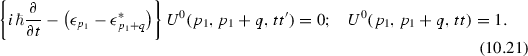
The solution of this commutator equation is

which, obviously, is related to the quasiparticle propagators (cf. Appendix D) simply by \(U^0(1,1+q,tt')=U_1(tt')\,U^{*}_{1+q}(tt')\).
- 9.
- 10.
Or, equivalently the longitudinal component of the electromagnetic field, see also Chap. 13.
- 11.
The ansatz (10.26) was only used for identical transformations.
- 12.
- 13.
- 14.
Modifications appear only in case of multiple time integrations. For example, the integral \(A(t_1t_2)\) splits in a sum of two according to
$$\begin{aligned} A(t_1t_2)= \int _{t_0}^{t_1}dt_3\int _{t_0}^{t_2}dt_4 B(t_1t_3)C(t_3t_4)D(t_4t_2) =\int _{t_0}^{t_1}dt_3\int _{t_0}^{t_2}dt_4 B^{+}(t_1t_3)C(t_3t_4)D^{-}(t_4t_2) \nonumber \\ =\int _{t_0}^{t_1}dt_3\int _{t_0}^{t_3}dt_4 B^{+}(t_1t_3)C^{+}(t_3t_4)D^{-}(t_4t_2) +\int _{t_0}^{t_1}dt_3\int _{t_3}^{t_2}dt_4 B^{+}(t_1t_3)C^{-}(t_3t_4)D^{-}(t_4t_2), \nonumber \end{aligned}$$where the resulting two integrals have a clear time ordering in all quantities.
- 15.
The transformations are analogous to the ones used to derive the non-Markovian Boltzmann collision integral, Chap. 9. The decomposition in the two integral terms in brackets arises from different time orderings in the \(t_3\) and \(t_4\) integrations as explained in footnote 13, see also [261]. The initial correlation term in (10.11) is treated analogously.
- 16.
The introduction of the retarded and advanced quantities was discussed at the end of Sect. 10.2. In particular, the explicit form of the propagators \(U^{0\pm }(tt')\) follows immediately from (10.22) by multiplication with \(\Theta [\pm (t-t')]\).
- 17.
In principle, the derivation yields the renormalized energies \(\epsilon \) in the denominator. However, this leads to inconsistencies, and the proper inclusion of renormalization effects is still being debated.
- 18.
Recall that all momenta have to be understood as vectors.
- 19.
To this end, we again have to use the limiting result (10.39) for the dielectric function, where the static long wavelength limit (\(\omega \rightarrow 0\) and, subsequently, \(q\rightarrow 0\)) has to be taken. As a result, in (10.44), the integrations over \(t_1\) and \(t_2\) are removed and the square of the statically screened Coulomb potential (Debye potential) appears.
- 20.
This assumes that the one-particle distributions are equilibrium (Fermi/Bose) distributions.
- 21.
More generally, one may wish to be able to consider also situations where already carriers, and thus, also correlations exist in the system prior to the onset of the excitation.
- 22.
Already in 1928 Debye and Falkenhagen calculated the relaxation time of the screening cloud around an ion if the ion is perturbed (removed), see also [138].


Author information
Authors and Affiliations
Corresponding author
Rights and permissions
Copyright information
© 2016 Springer International Publishing Switzerland
About this chapter
Cite this chapter
Bonitz, M. (2016). \(*\)Random Phase Approximation. In: Quantum Kinetic Theory. Springer, Cham. https://doi.org/10.1007/978-3-319-24121-0_10
Download citation
DOI: https://doi.org/10.1007/978-3-319-24121-0_10
Published:
Publisher Name: Springer, Cham
Print ISBN: 978-3-319-24119-7
Online ISBN: 978-3-319-24121-0
eBook Packages: Physics and AstronomyPhysics and Astronomy (R0)