
Abstract
In this chapter we give a short account of the Lagrangian and Hamiltonian formulation of classical non-relativistic and relativistic theories. For pedagogical reasons we first address the case of systems of particles, described by a finite number of degrees of freedom. Afterwards, starting from Sect. 8.5, we extend the formalism to fields, that is to dynamical quantities described by functions of the points in space. Their consideration implies the study of dynamical systems carrying a continuous infinity of canonical coordinates, labeled by the three spatial coordinates.
Access this chapter
Tax calculation will be finalised at checkout
Purchases are for personal use only
Notes
- 1.
Here and in the following we shall often use the shorter notation q(t) for the set of the coordinates \(\{q_i\}=(q_1,\dots ,q_n)\) and similarly for their time derivatives, \(\dot{q}=\{\dot{q}_i\}=(\dot{q}_1,\dots ,\dot{q}_n)\).
- 2.
To avoid clumsiness in the following formulae we shall often adopt the Einstein convention of summing over repeated indices \(i,j,\dots \) of the Lagrangian coordinates, even though these indices are in general just suffixes with no tensorial property.
- 3.
Note that the function f can depend on \(q_i\) and t only, \(f=f(q,t)\), in order for df / dt not to depend on derivatives of \(q_i\) of order higher than one.
- 4.
We can directly show that the presence of an additional total derivative does not affect the equations of motion by showing that df / dt identically satisfies Eq. (8.7). This is readily done by observing that
$$ {\frac{df}{dt}(q,\dot{q},t)=\dot{q}_i\,\frac{\partial f}{\partial q_{i}}+\frac{\partial f}{\partial t},} $$so that
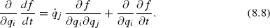
On the other hand we have

Subtracting side by side Eq. (8.8) from Eq. (8.9) and using the property that the partial derivations with respect to \(q_i\) and t commute, we conclude that the Euler-Lagrange equations are identically satisfied by the total derivative.
- 5.
This last property gives a physical meaning to our definition of inertial mass m. Indeed, the multiplication by a constant does not change the equations of motion, but it is equivalent to a change of the mass unit in the Lagrangian (8.12). However all the mass ratios, having a physical meaning, are unchanged.
- 6.
The number of degrees of freedom of the system is \(n=3N\).
- 7.
The proof in a more general case is given in the following subsection.
- 8.
With an abuse of notation, we shall use the same Latin indices \(i, j, k,\dots \) to label the three-dimensional Euclidean coordinates \(x^i\) and the generalized coordinates \(q^i\), though the reader should bear in mind that in the latter case they run over the total number n of degrees of freedom of the system. Moreover the index k, when written within brackets, is also used to label the particle in the system. The meaning of these indices will be clear form the context.
- 9.
Note that since we have assumed \(\frac{\partial L}{\partial t}=0\) we have \(\dot{U}=0\), meaning that our system is isolated.
- 10.
As noted in the previous discussion invariance under transformations parametrized by just some components of the vector parameters \({\varvec{\epsilon }}\) and \(\delta \varvec{\theta }\), implies the conservation of the corresponding components of the vector quantities \(\mathbf {P}\) and \(\mathbf {M}\).
- 11.
From the Hamiltonian point of view we must substitute \(v^2= \frac{c^2|\mathbf{p}|^2}{c^2m^2+|\mathbf{p}|^2}\).
- 12.
Note that the transformations (8.81) form a group, the group of coordinate transformations in phase space.
- 13.
We do not consider in this case transformation of the time variable.
- 14.
In this subsection we use the notations \(p'_i, q'_i\) instead of \(P_i,Q_i\).
- 15.
More precisely, since \(\mathbf {x}\equiv (x^1,x^2,x^3)\), we have a triple infinity of Lagrangian coordinates \(q_i(t)\) for each value of the index \(\mu =0,1,2,3\). The three components of \(\mathbf {x}\) and the index \(\mu \) play the role of the index i of the discrete case.
- 16.
Actually in our treatment of a discrete number of degrees of freedom, we have often omitted the symbol \(\varSigma \) when there were repeated indices.
- 17.
Somewhat improperly, by the word representation people often refer to the carrier space \(V_p\) of a representation. We shall also do this to simplify the exposition and thus talk about a basis of a representation when referring to a basis of the corresponding carrier space.
- 18.
This is true if the boundary \(\partial D_4\) does not extend to spatial infinity; when the integration domain \(D_4\) fills the whole space, we must require that the fields and their derivatives fall off sufficiently fast at infinity, or we may also use periodic boundary conditions. In any case the integration on an infinite domain can always be taken initially on a finite domain, and, after removing the boundary term, the integration domain can be extended to infinity.
- 19.
Recall that the latter tensor \(\epsilon _{\mu \nu \rho \sigma }\) is not invariant under Lorentz transformations which are in \(\mathrm{O}(1,3)\) but not in \(\mathrm{SO}(1,3)\), namely which have determinant \(-1\). Examples of these are the parity transformation \(\varvec{\Lambda }_P\), or time reversal \(\varvec{\Lambda }_T\).
- 20.
Note that the kinetic term for \(A_0\) is absent because of the antisymmetry of \(F_{\mu \nu }\).
- 21.
Note that we are describing the interaction of the electromagnetic field, possessing infinite degrees of freedom, with a system of N charged particles, having 3N degrees of freedom represented by the N coordinate vectors \(\mathbf {x}_{(k)}(t), (k=i,\dots , N)\). The Dirac delta function formally converts the 3N degrees of freedom of \(\mathbf {x}_{(k)}(t)\) into the infinite degrees of freedom associated to \(\mathbf {x}\).
- 22.
Note that this condition just fixes the charge normalization.
- 23.
The index k given to \(\mathbf {x}_{(k)}\) in the following formulae has the function of indicating that the coordinate vector \(\mathbf {x}_{(k)}(t)\) is a dynamical variable, and not the labeling of the space points, as is the case for \(\mathbf {x}\).
- 24.
Note that also \({\mathcal S}_{part}\) can be written as a four-dimensional integral:
$$ \mathcal S_{int}= -\sum \limits _k m_kc \int d^4x \,\delta ^{(3)}(\mathbf {x}-{\mathbf {x}}_{(k)})\left( 1-\frac{1}{c^2}\left( \frac{d\mathbf {x}}{dt}\right) ^2\right) . $$.
- 25.
Here and in the following we use the subscript 0 to denote the usual free-particle momentum \(p_{(0)}^i=m(v)v^i\) and the symbol \(p^i\) for the momentum canonically conjugated to \(x^i\).
- 26.
Recall that the vector \(\mathbf{A}\equiv (A_i)\) is the spatial part of the four-vector \(A_\mu \equiv (A_0,\,\mathbf{A})\), so that \(A^\mu \equiv (A_0,\,-\mathbf{A})\). On the other hand \(\mathbf{p}\) is the spatial component of \(p^\mu \equiv (p^0,\mathbf{p})\), so that \(p_\mu \equiv (p^0,-\mathbf{p})\).
- 27.
We note that the invariance of the action means that two configurations \( \left[ \varphi ^{\alpha }(x),\,x^{\mu }\,\in \, D_4\right] \) and \( \left[ \varphi ^{\prime \alpha }(x'),x'^{\mu }\,\in \,D'_4\right] \) related by the transformation (8.145) are solutions to the same partial differential equations.
- 28.
This freedom will be taken into account when discussing the energy momentum tensor in the next section.
- 29.
The alternative name of stress-energy tensor is also used.
- 30.
We shall illustrate an application of this mechanism to the case of the electromagnetic field at the end of this section.
- 31.
- 32.
Recall from Chap. 4 that, since \(L_{\rho \sigma }\) are Lorentz generators, \(L_i=-\epsilon _{ijk}L_{jk}/2\) are generators of the rotation group.


Author information
Authors and Affiliations
Corresponding author
Rights and permissions
Copyright information
© 2016 Springer International Publishing Switzerland
About this chapter
Cite this chapter
D’Auria, R., Trigiante, M. (2016). Lagrangian and Hamiltonian Formalism. In: From Special Relativity to Feynman Diagrams. UNITEXT for Physics. Springer, Cham. https://doi.org/10.1007/978-3-319-22014-7_8
Download citation
DOI: https://doi.org/10.1007/978-3-319-22014-7_8
Published:
Publisher Name: Springer, Cham
Print ISBN: 978-3-319-22013-0
Online ISBN: 978-3-319-22014-7
eBook Packages: Physics and AstronomyPhysics and Astronomy (R0)