Analyzing Dyadic Data with IRT Models

Abstract

Dyadic data frequently occur in social sciences and numerous techniques have been developed for their analysis. The most prominent methods involve using regression, path, and structural equation models. The present contribution extends these approaches by considering Item Response Theory (IRT) Models. Two pivotal dyadic data analysis models, the Actor-Partner Interdependence Model (APIM) and the Common Fate Model (CFM), are built using the Multidimensional Random Coefficients Multinomial Logit Model (MRCMLM). This approach combines the advantages of dyadic data analysis with a model for discrete data, thus allowing for categorical items while drawing inferences based on the estimated true scores on an interval scale.

Appendices

Technical Appendix: APIM Commands

Table 1 Description of ConQuest commands regarding the APIM

APIM Item Fit Indices

Listing 8 Item Fit Indices for the APIM

item::

Item number and label; as no label has been provided, the item number is repeated.

ESTIMATE::

Item parameter estimate; in the dichotomous case, this is the item difficulty parameter [δ _i according to Eq. (1)]. To identify a latent scale, one item per latent dimension is fixed (indicated by an asterisk). By default, ConQuest sets the sum of the item parameters per latent dimension to zero (e.g.: − 1. 452 + 0. 688 + 0. 137 + 0. 147 + (−0. 124) +0.604 = 0). This could be overridden with the command set constraint=cases, causing the mean of the latent variable to be fixed at zero.

ERROR::

Standard error of item difficulty parameter.

MNSQ::

Outfit (UNWEIGHTED FIT) and Infit (WEIGHTED FIT) Index.

CI::

The 95 % confidence interval for the expected value (i.e., 1) of Infit and Outfit.

T::

The t-statistic for the null hypothesis that the Outfit and Infit Index is 1. Values larger than 2 may be considered significant at the 95 % level (corresponds to MNSQ outside the CI).

Extracting the Individual Level Correlation Coefficients

To obtain the individual level correlation coefficients, we use the residuals stored in resid.txt. This file contains 600 lines and 25 columns. The first column is a numerical dyad identifier, followed by four groups of six columns each, comprising the residuals to the respective six items of student/self, student w.r.t parent, parent/self and parent w.r.t student. Any multi-purpose statistics software can be used to obtain the individual level correlation coefficients. We will resort to the R software (R Core Team 2014) for it is freely available (open source) and easy to use. The following script will perform the required steps:

Listing 9 R Script for Computing the CFM Individual Level Correlation Coefficients

The ten statements of Listing 9 perform the following operations:

• In line 1 of the script, we read the content of the file resid.txt and store it in a data.frame named d0.

• Then (line 2) we transform the missing values (ConQuest codes them with -99 by default) to the R missing indicator NA.

• In lines 3–6, the columns obtain more informative variable names (the output file contains no header, therefore, R uses the generic names V1 to V25 by default). This step is merely cosmetic and may as well be omitted.

• Next (line 8), we compute the 25 × 25 correlation matrix of all residuals (omitting the id variable stored in column 1). A schematic view of this matrix is given in Fig. 8.

  Fig. 8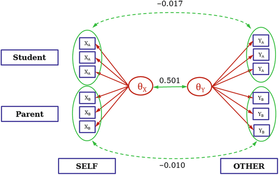

  

  The final CFM

• In line 10, we cut out blocks of correlation coefficients of the residuals of the students’ self-description items with the columns covering the residuals of the students’ assessments of the respective parents (rows 1–6/columns 7–12; grey shaded area termed rA in Fig. 8).

• Analoguously, in line 11, we cut out the correlation coefficients of the residuals of the parents’ self-assessment items with the residuals of the items covering the parents’ assessments of the respective students (rows 13–18/columns 19–24; grey shaded area termed rB in Fig. 8).

• In lines 13 and 14 we prepare two functions, transforming a correlation coefficient to a Fisher’s Z-value (r2z) and backtransforming the latter into a correlation coefficient again (z2r). These functions could easily be enhanced to detect invalid input and issue a corresponding message.

• Finally (lines 16 and 17), we apply the Z-transformation to the two matrix parts, compute the mean and backtransform it to a valid correlation coefficient.

With these steps, we dispose of all required information to draw the complete CFM, depicted in Fig. 7.

CFM Item Fit Indices

Listing 10 Item Fit Indices for the CFM

For an explanation of the column headings see Appendix “APIM Item Fit Indices”.

References

Adams, R. J., Wilson, M., & Wang, W.-C. (1997). The multidimensional random coefficients multinomial logit model. Applied Psychological Measurement, 21, 1–23.
Adams, R. J., & Wu, M. L. (2007). The mixed-coefficients multinomial logit model: A generalized form of the rasch model. In M. von Davier & C. H. Carstensen (Eds.), Multivariate and mixture distribution Rasch models. Extensions and applications (pp. 57–75). New York, NY: Springer.
Adams, R. J., Wu, M. L., & Wilson, M. (2012). Conquest 3.0 [Computer software]. Melbourne: Australian Council for Educational Research (ACER).
Andersen, E. B. (1970). Asymptotic properties of conditional maximum likelihood estimators. Journal of the Royal Statistical Society, Series B, 32, 283–301.
Andersen, E. B. (1973). A goodness of fit test for the Rasch model. Psychometrika, 38, 123–140.
Andersen, E. B. (1977). Sufficient statistics and latent trait models. Psychometrika, 42, 69–81.
Andersen, E. B. (1980). Discrete statistical models with social science applications. Amsterdam: North-Holland.
Andrich, D. (1978). A rating formulation for ordered response categories. Psychometrika, 43, 561–573.
Andrich, D. (1982). An extension of the Rasch Model for ratings providing both location and dispersion parameters. Psychometrika, 47, 105–113.
Baker, F. B., & Kim, S.-H. (2004). Item response theory. Parameter estimation techniques. New York, NY: Marcel Dekker.
Baumeister, R. R., Dale, K., & Sommer, K. L. (1998). Freudian defense mechanisms and empirical findings in modern social psychology: Reaction formation, projection, displacement, undoing, isolation, sublimation, and denial. Journal of Personality, 66, 1081–1124.
Beckmann, D., Bräahler, E., & Richter, H.-E. (1990). Der Gießen-Test (GT). Ein Test für Individual- uind Gruppendiagnostik [The Gießen test (GT). A test for the assessment of individuals and groups] (4th ed.). Bern: Hans Huber.
Birnbaum, A. (1968). Some latent trait models and their use in inferring an examinee’s ability. In F. M. Lord & M. E. Novick (Eds.), Statistical theories of mental test scores with contributions by A. Birnbaum (pp. 395–479). Reading, MA: Addison-Wesley.
Blanca, M. J., Arnau, J., López-Montiel, D., Bono, R., & Bendayan, R. (2013). Skewness and kurtosis in real data samples. Methodology, 9, 78–84.
Bollen, K. A. (1989). Structural equations with latent variables. Hoboken, NJ: Wiley.
Bollen, K. A., & Barb, K. H. (1981). Pearson’s r and coarsely categorized measures. American Sociological Review, 46, 232–239.
Campbell, D. T. (1958). Common fate, similarity, and other indices of the status of aggregates of persons as social entities. Behavioral Science, 3, 14–25.
Campbell, L., & Kashy, D. A. (2002). Estimating actor, partner, and interaction effects for dyadic data using PROC MIXED and HLM: A guided tour. Personal Relationship, 9, 327–342.
Choi, J., Peters, M., & Mueller, R. O. (2010). Correlational analysis of ordinal data: From Pearson’s r to Bayesian polychoric correlation. Asia Pacific Educational Review, 11, 459–466.
Gebhardt, E. C. (in preparation). Latent Path Models within an IRT Framework. Unpublished doctoral dissertation, University of Melbourne, Melbourne, Australia.
de Ayala, R. J. (2009). The theory and practice of item response theory. New York, NY: Guilford.
Fischer, G. H. (1973). The linear logistic test model as an instrument in educational research. Acta Psychologica, 37, 359–374.
Fischer, G. H. (1995). The linear logistic test model. In G. H. Fischer & I. W. Molenaar (Eds.), Rasch models. Foundations, recent developments, and applications (pp. 131–155). New York, NY: Springer.
Freud, S. (1976). In J. Strachey (Ed.), The complete psychological works of Sigmund Freud (The standard edition). New York, NY: W. W. Norton & Company.
Glas, C. A. W., & Verhelst, N. D. (1995). Testing the Rasch model. In G. H. Fischer & I. W. Molenaar (Eds.), Rasch models. Foundations, recent developments, and applications (pp. 69–95). New York, NY: Springer.
Hox, J. J. (2010). Multilevel analysis. Techniques and applications (2nd ed.). New York, NY/Hove: Routledge.
Kenny, D. A., Kashy, D. A., & Cook, W. L. (2006). Dyadic data analysis. New York, NY: Guilford.
Kenny, D. A., & Ledermann, T. (2010). Detecting, measuring, and testing dyadic patterns in the actor-partner interdependence model. Journal of Family Psychology, 24, 359–366.
Linacre, J. M. (1989). Multi-facet Rasch measurement. Chicago, IL: Mesa Press.
Loeys, T., Cook, W., De Smet, O., Wietzker, A., & Buysse, A. (2014). The actor-partner interdependence model for categorical dyadic data: A user-friendly guide to GEE. Personal Relationships, 21, 225–241.
Loeys, T., & Molenberghs, G. (2013). Modeling actor and partner effects in dyadic data when outcomes are categorical. Psychological Methods, 18, 220–236.
Lord, F. M. (1980). Applications of item response theory to practical testing problems. Hillsdale, NJ: Lawrence Erlbaum Associates.
Masters, G. N. (1982). A Rasch model for partial credit scoring. Psychometrika, 47, 149–174.
McMahon, J. M., Puget, E. R., & Tortu, S. (2006). A guide for multilevel modeling of dyadic data with binary outcomes using SAS PROC NLMIXED. Computational Statistics & Data Analysis, 50, 3663–3680.
Micceri, T. (1989). The unicorn, the normal curve, and other improbable creatures. Psychological Bulletin, 105, 156–166.
Monin, B., & Oppenheimer, D. M. (2005). Correlated averages vs. averaged correlations: Demonstrating the warm glow heuristic beyond aggregations. Social Cognition, 23, 257–278.
Müller, H. (1987). A rasch model for continuous ratings. Psychometrika, 52, 165–181.
Muthén, B. (1984). A general structural equation model with dichotomous, ordered categorical and continuous latent variable indicators. Psychometrika, 49, 115–132.
Neyman, J., & Scott, E. L. (1948). Consistent estimates based on partially consistent observations. Econometrica, 16, 1–32.
R Core Team. (2014). R: A language and environment for statistical computing [Computer software manual], Vienna, Austria. Retrieved from http://www.R-project.org
Rasch, G. (1960). Probabilistic models for some intelligence and attainment tests. Copenhagen: Danmarks Pædagogiske Institut.
Rasch, G. (1961). On general laws and the meaning of measurement in psychology. Copenhagen: The Danish Institute of Educational Research.
Rasch, G. (1977). On specific objectivity: an attempt at formalizing the request for generality and validity of scientific statements. Danish Yearbook of Philosophy, 14, 58–93.
Rasch, G. An informal report on the present state of a theory of objectivity in comparisons. In Proceedings of the NUFFIC International Summer Session in Science at “Het Oude Hof”, The Hague, 14–28, July, 1966. Retrieved July 22, 2015, from http://www.rasch.org/memo1966.pdf.
Reckase, M. D. (2009). Multidimensional item response theory. New York, NY: Springer.
Stock, J. H., & Trebbi, F. (2003). Who invented instrumental variable regression? Journal of Economic Perspectives, 17, 177–194.
van der Linden, W. J., & Hambleton, R. K. (Eds.). (1997). Handbook of modern item response theory. New York, NY: Springer.
von Eye, A., & Mun, E.-Y. (2013). Log-linear modeling: Concepts, interpretation, and application. Hoboken, NJ: Wiley.
Wright, B. D., & Masters, G. N. (1982). Rating scale analysis. Chicago, IL: Mesa Press.
Wright, B. D., & Stone, M. H. (1979). Best test design. Chicago, IL: Mesa Press.
Wu, M. L., Adams, R. J., Wilson, M. R., & Haldane, S. A. (2007). ACER ConQuest. Generalised item response modelling software. Melbourne: ACER Press.
Acknowledgements
I am indebted to Paul Czech for his assistance during data acquisition of the students’ sample.
Author information
Authors and Affiliations
Corresponding author
Editor information
Editors and Affiliations