Variational Bayes for Hierarchical Mixture Models

Abstract

In recent years, sparse classification problems have emerged in many fields of study. Finite mixture models have been developed to facilitate Bayesian inference where parameter sparsity is substantial. Classification with finite mixture models is based on the posterior expectation of latent indicator variables. These quantities are typically estimated using the expectation-maximization (EM) algorithm in an empirical Bayes approach or Markov chain Monte Carlo (MCMC) in a fully Bayesian approach. MCMC is limited in applicability where high-dimensional data are involved because its sampling-based nature leads to slow computations and hard-to-monitor convergence. In this chapter, we investigate the feasibility and performance of variational Bayes (VB) approximation in a fully Bayesian framework. We apply the VB approach to fully Bayesian versions of several finite mixture models that have been proposed in bioinformatics, and find that it achieves desirable speed and accuracy in sparse classification with finite mixture models for high-dimensional data.

Appendix: The VB-LEMMA Algorithm

1.1 The B-LEMMA Model

We consider a natural extension to the LEMMA model in Bar et al. (2010): a fully Bayesian three-component mixture model, B-LEMMA:

$$\displaystyle \begin{aligned} d_g | (b_{1g}, b_{2g}), \psi_{g}, \sigma^2_{\epsilon,g}, \tau &= \tau + (b_{1g} - b_{2g}) \psi_{g} + \epsilon_{g} \\ m_g | \sigma^2_{\epsilon,g} &\sim \frac{{\sigma^2_{\epsilon,g}}{{\chi}^2_{f_g}}}{f_g}, \quad \text{where } f_g := n_{1g}+n_{2g}-2 \\ \psi_g | \psi, \sigma^2_\psi &\sim N(\psi, \sigma^2_\psi) \quad i.i.d.\\ \epsilon_{g} | \sigma^2_{\epsilon,g} &\sim N(0, \sigma^2_g), \quad \text{where }\sigma^2_g := \sigma^2_{\epsilon,g}c_g, \\ & \qquad c_g := \frac{1}{n_{1g}}+ \frac{1}{n_{2g}} \\ ({b_{1g}},{b_{2g}},1-{b_{1g}}-{b_{2g}}) | (p_1,p_2) &\sim {\mathrm{Multinomial}}\left(1;p_1,p_2,1-p_1-p_2\right) \quad i.i.d.\\ \tau &\sim N\left(\mu_{\tau_0}, \sigma^2_{\tau_0} \right)\\ \psi &\sim N\left(\mu_{\psi_0}, \sigma^2_{\psi_0} \right)\\ \sigma_\psi^2 &\sim {\mathrm{IG}}\left(A_\psi,B_\psi\right)\\ \sigma^2_{\epsilon,g} &\sim {\mathrm{IG}}\left(A_\epsilon, B_\epsilon \right) \quad i.i.d.\\ \left(p_1,p_2,1-p_1-p_2\right) &\sim {\mathrm{Dirichlet}}\left(\alpha_1,\alpha_2,\alpha_0\right), \end{aligned} $$

where (b _1g, b _2g) takes values (1, 0), (0, 1), or (0, 0), indicating that gene g is in non-null group 1, non-null group 2, or null group, respectively. p ₁ and p ₂ are proportions of non-null group 1 and non-null group 2 genes. Hence, the non-null proportion is p ₁ + p ₂. Each of τ and ψ _g represents the same quantity as in the B-LIMMA model.

1.1.1 Algorithm

The VB-LEMMA algorithm was derived based on an equivalent model to B-LEMMA. In the equivalent model, the gene-specific treatment effect is treated as the combination of a fixed global effect and a random zero-mean effect. That is, conditional distribution of d _g and that of ψ _g are replaced with

$$\displaystyle \begin{aligned} d_g | (b_{1g}, b_{2g}), u_{g}, \sigma^2_{\epsilon,g}, \tau &= \tau + (b_{1g} - b_{2g}) \psi + (b_{1g} + b_{2g}) u_{g} + \epsilon_{g}\\ u_g | \sigma^2_\psi &\sim N(0, \sigma^2_\psi) \quad i.i.d. \end{aligned} $$

The set of observed data and the set of unobserved data are identified as

$$\displaystyle \begin{aligned} \mathbf{y} &= \{ \{d_g\}, \{m_g\} \} \\ H &= \{ \{\boldsymbol{b}_g\}, \{u_g\}, \{\sigma^2_g\}, \tau, \psi, \sigma^2_\psi, \boldsymbol{p} \} \end{aligned} $$

where b _g = (b _1g, b _2g) and p = (p ₁, p ₂).

Because of the similarities of the B-LEMMA model to the B-LIMMA model, derivation of VB-LEMMA was achieved by extending the derivation of VB-LIMMA that involves a gene-specific zero-mean random effect parameter. The VB algorithm based on the exact B-LEMMA model was also derived for comparison. However, little discrepancy in performance between the VB algorithm based on the exact model and VB-LEMMA was observed. Therefore, VB-LEMMA based on the equivalent model was adopted.

The product density restriction

$$\displaystyle \begin{aligned} {q}(H) &= q_{\{\boldsymbol{b}_g\}} (\{\boldsymbol{b}_g\}) \times q_{\{\psi_g\}} (\{\psi_g\}) \times q_{\{\sigma^2_g\}} (\{\sigma^2_g\}) \times q_{(\tau, \boldsymbol{p})}(\tau, \boldsymbol{p}) \times q_{(\psi, \sigma^2_\psi)}(\psi, \sigma^2_\psi) \end{aligned} $$

leads to q-densities

$$\displaystyle \begin{aligned} q_\tau (\tau) &= N \left( \widehat{M_\tau},\widehat{V_\tau} \right) \\ q_\psi (\psi ) &= N \left( \widehat{M_{\psi}},\widehat{V_{\psi}} \right) \\ q_{\sigma_g^{2}} (\sigma_g^{2}) &= {\mathrm{IG}} \left( A_{\sigma_g^{2}},\widehat{B_{\sigma_g^{2}}} \right) \\ q_{\left({b_{1g}},{b_{2g}},1-{b_{1g}}-{b_{2g}}\right)} (\left({b_{1g}},{b_{2g}},1-{b_{1g}}-{b_{2g}}\right)) &= {\mathrm{Multinomial}} \left( \widehat{M_{b_{1g}}}, \widehat{M_{b_{2g}}}, \right.\\ &\quad \left. 1-\widehat{M_{b_{1g}}}-\widehat{M_{b_{2g}}}\right) \\ q_{\left(p_1,p_2,1-p_1-p_2\right)} (\left(p_1,p_2,1-p_1-p_2\right)) &= {\mathrm{Dirichlet}} \left( \widehat{\alpha_{p_1}}, \widehat{\alpha_{p_2}}, \widehat{\alpha_{p_0}}\right) \\ q_{\sigma_\psi^{2}} (\sigma_\psi^{2}) &= {\mathrm{IG}}\left( A_{\sigma_\psi^{2}},\widehat{B_{\sigma_\psi^{2}}} \right). \end{aligned} $$

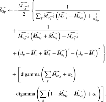
It is only necessary to update the variational posterior means $\hat {M_\cdot }$ in VB-LEMMA. Upon convergence, the other variational parameters are computed based on the converged value of those involved in the iterations. The iterative scheme is as follows:

• 1. Initialize

  $$\displaystyle \begin{aligned} \widehat{M_{\sigma_\psi^{-2}}} &=1\\ \widehat{M_{\sigma_g^{-2}}} &=\frac{1}{c_g}\;\forall\: g \\ \widehat{M_{b_g}} &= \left\{ \begin{array}{l l} (1,0,0) & \quad \text{if rank{$(d_g) \geq (1-0.05)G$}}\\ (0,1,0) & \quad \text{if rank{$(d_g) \leq 0.05G$}}\\ (0,0,1) & \quad \text{otherwise} \end{array} \right. \text{ for each } g \\ \widehat{M_\psi} &= \frac{1}{2}\left(\bigg \vert \sum_{\{g: \text{rank}(d_g) \geq (1-0.05)G\}}{d_g} - \sum_{g=1}^G{d_g}\bigg \vert+\bigg \vert \sum_{g=1}^G{d_g} - \sum_{\{g: \text{rank}(d_g) \leq 0.05G\}}{d_g} \bigg \vert \right) \\ \widehat{M_{u_g}} &= 0\;\forall\: g \\ \text{Set } A_{\sigma_\psi^2}&=\frac{G}{2}+A_\psi \quad \text{and}\quad A_{\sigma_g^2}=\frac{1+f_g}{2}+A_\varepsilon \;\text{for each}\;g. \end{aligned} $$

• 2. Update

  $$\displaystyle \begin{aligned} \widehat{M_\tau} \; & \leftarrow\; \left\{ \sum_{g} \widehat{M_{\sigma_g^{-2}}}\left[ \left(1-\widehat{M_{b_{1g}}}-\widehat{M_{b_{2g}}} \right)d_g + \widehat{M_{b_{1g}}}\left(d_g-\widehat{M_\psi}-\widehat{M_{u_g}}\right) \right. \right. \\ & \qquad \left. \left. + \widehat{M_{b_{2g}}} \left(d_g+\widehat{M_\psi}-\widehat{M_{u_g}}\right)\right] + \frac{\mu_{\tau_0}}{\sigma^2_{\tau_0}}\right\} \times \dfrac{1}{ \sum_{g}\widehat{M_{\sigma_g^{-2}}} + \frac{1}{\sigma^2_{\tau_0}}} \\ \widehat{M_{\psi}} \; & \leftarrow\; \left\{ \sum_{g} \widehat{M_{\sigma_g^{-2}}} \left( \widehat{M_{b_{1g}}} - \widehat{M_{b_{2g}}} \right) \left(d_g-\widehat{M_\tau}-\widehat{M_{u_g}}\right) + \frac{\mu_{\psi_0}}{\sigma^2_{\psi_0}}\right\} \\ & \qquad \times \dfrac{1}{ \sum_{g}\widehat{M_{\sigma_g^{-2}}}\left(\widehat{M_{b_{1g}}}+\widehat{M_{b_{2g}}}\right)+\frac{1}{\sigma^2_{\psi_0}}} \\ \widehat{M_{u_g}} \; & \leftarrow\; \widehat{M_{\sigma_g^{-2}}}\left[ \widehat{M_{b_{1g}}}\left(d_g-\widehat{M_\tau}-\widehat{M_\psi}\right) + \widehat{M_{b_{2g}}} \left(d_g-\widehat{M_\tau}+\widehat{M_\psi}\right)\right]\\ & \qquad \times \dfrac{1}{\widehat{M_{\sigma_g^{-2}}}\left(\widehat{M_{b_{1g}}}+\widehat{M_{b_{2g}}}\right)+\widehat{M_{\sigma_\psi^{-2}}} } \end{aligned} $$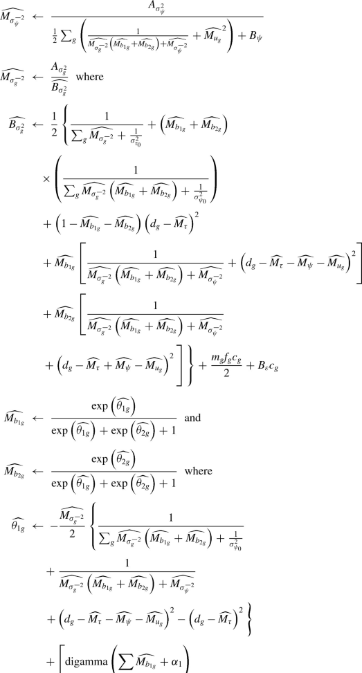
  
  

• 3. Repeat (2) until the increase in

  $$\displaystyle \begin{aligned} & \log\underline{p} \left(\mathbf{y};\mathbf{q}\right) \\ &\quad = \frac{-G}{2}\times\log{\left(2\pi\right)} -\sum_g \left[\widehat{M_{b_{1g}}}\log{\widehat{M_{b_{1g}}}}+\widehat{M_{b_{2g}}}\log{\widehat{M_{b_{2g}}}} \right.\\ &\qquad \left. +\left(1-\widehat{M_{b_{1g}}}-\widehat{M_{b_{2g}}}\right)\log{\left(1-\widehat{M_{b_{1g}}}-\widehat{M_{b_{1g}}}\right)}\right] \\ &\qquad +\log{\left( {\mathrm{Beta}} \left(\sum_{g}\widehat{M_{b_{1g}}}+\alpha_1,\sum_{g}\widehat{M_{b_{2g}}}+\alpha_2,\sum_{g}\left(1-\widehat{M_{b_{1g}}}-\widehat{M_{b_{2g}}}\right)+\alpha_0\right)\right)} \\ & \qquad - \log{\left( {\mathrm{Beta}} \left(\alpha_1,\alpha_2,\alpha_0\right)\right)} \\ & \qquad +\left[\log{\left(\frac{1}{ \sum_{g}\widehat{M_{\sigma_g^{-2}}} + \frac{1}{\sigma^2_{\tau_0}}}\right)}\right.\\ &\qquad \left.-\log{{\sigma^2_{\tau_0}}}+1-\dfrac{\frac{1}{ \sum_{g}\widehat{M_{\sigma_g^{-2}}} + \frac{1}{\sigma^2_{\tau_0}}}+\left(\widehat{M_\tau}-\mu_{\tau_0}\right)^2}{\sigma^2_{\tau_0}}\right]\times\frac{1}{2}\\ & \qquad +\left[\log{\left(\frac{1}{\sum_{g}\widehat{M_{\sigma_g^{-2}}}\left(\widehat{M_{b_{1g}}}+\widehat{M_{b_{2g}}}\right)+\frac{1}{\sigma^2_{\psi_0}}} \right)}-\log{{\sigma^2_{\psi_0}}}\right]\times\frac{1}{2} \\ & \qquad +\left[1-\dfrac{\left(\frac{1}{\sum_{g}\widehat{M_{\sigma_g^{-2}}}\left(\widehat{M_{b_{1g}}}+\widehat{M_{b_{2g}}}\right)+\frac{1}{\sigma^2_{\psi_0}}} \right)+\left(\widehat{M_\psi}-\mu_{\psi_0}\right)^2}{\sigma^2_{\psi_0}}\right]\times\frac{1}{2} \\ &\qquad +G\times{A_\varepsilon}\log{B_\varepsilon}+\sum_g \left[\left(\frac{f_g}{2}+A_\varepsilon\right)\log{c_g}\log{\Gamma{\left(A_{\sigma_g^{2}}\right)}}-\log{\Gamma{\left(A_\varepsilon\right)}}\right. \\ &\qquad +\left. -\frac{f_g}{2}\log{2}-\log{\Gamma{\left(\frac{f_g}{2}\right)}}+\left(\frac{f_g}{2}-1\right)\log{m_g}+\frac{f_g}{2}\log{f_g}\right] \\ &\qquad +\sum_g \left\{ \frac{A_{\sigma_g^{2}}}{\widehat{B_{\sigma_g^{2}}}}\times \left[ -\frac{1}{2}{m_g}{f_g}{c_g}-{B_\varepsilon}{c_g} \right. \right. \\ &\qquad - \left. \left. {\frac{1}{2}}\left(\frac{1}{ \sum_{g}\widehat{M_{\sigma_g^{-2}}} + \frac{1}{\sigma^2_{\tau_0}}}+\left(1-\widehat{M_{b_{1g}}}-\widehat{M_{b_{2g}}}\right)\left({d_g}-\widehat{M_\tau}\right)^2\right)\right. \right. \\ &\qquad - \left. \left. \frac{\widehat{M_{b_{1g}}} + \widehat{M_{b_{1g}}}}{2}\left(\frac{1}{\sum_{g}\widehat{M_{\sigma_g^{-2}}}\left(\widehat{M_{b_{1g}}}+\widehat{M_{b_{2g}}}\right)+\frac{1}{\sigma^2_{\psi_0}}}\right)\right. \right. \\ & \qquad - \left. \left.\frac{\widehat{M_{b_{1g}}}}{2}\left(\frac{1}{\widehat{M_{\sigma_g^{-2}}}\left(\widehat{M_{b_{1g}}}+\widehat{M_{b_{2g}}}\right)+\widehat{M_{\sigma_\psi^{-2}}} }+\left({d_g}-\widehat{M_\tau}-\widehat{M_\psi}-\widehat{M_{u_g}}\right)^2\right) \right. \right. \\ & \qquad - \left. \left.\frac{\widehat{M_{b_{2g}}}}{2}\left(\frac{1}{\widehat{M_{\sigma_g^{-2}}}\left(\widehat{M_{b_{1g}}}+\widehat{M_{b_{2g}}}\right)+\widehat{M_{\sigma_\psi^{-2}}} }+\left({d_g}-\widehat{M_\tau}+\widehat{M_\psi}-\widehat{M_{u_g}}\right)^2\right) \right] \right\} \\ &\qquad + \sum_g{{A_{\sigma_g^{2}}\left(-\log{\widehat{B_{\sigma_g^{2}}}}+1\right) }} \\\noalign{} &\qquad + \frac{1}{2}\sum_g{\left[\log\left( \frac{1}{\widehat{M_{\sigma_g^{-2}}}\left(\widehat{M_{b_{1g}}}+\widehat{M_{b_{2g}}}\right) +\widehat{M_{\sigma_\psi^{-2}}} } \right)+1\right]} \\ & \qquad +{A_\psi}\log{B_\psi}-\log{\Gamma{\left(A_\psi\right)}} + {A_{\sigma_\psi^{2}}\left(-\log{\widehat{B_{\sigma_\psi^{2}}}}\right) }+\log{\Gamma{\left(A_{\sigma_\psi^{2}}\right)}} \end{aligned} $$

  from previous iteration becomes negligible.

• 4. Upon convergence, the remaining variational parameters are computed:

  $$\displaystyle \begin{aligned} \widehat{V_\tau} &\leftarrow\; \dfrac{1}{ \sum_{g}\widehat{M_{\sigma_g^{-2}}} + \frac{1}{\sigma^2_{\tau_0}}} \\ \widehat{V_{\psi}} &\leftarrow\; \dfrac{1}{\sum_{g}\widehat{M_{\sigma_g^{-2}}}\left(\widehat{M_{b_{1g}}}+\widehat{M_{b_{2g}}}\right)+\frac{1}{\sigma^2_{\psi_0}}} \\ \widehat{V_{u_g}} &\leftarrow\; \dfrac{1}{\widehat{M_{\sigma_g^{-2}}}\left(\widehat{M_{b_{1g}}}+\widehat{M_{b_{2g}}}\right)+\widehat{M_{\sigma_\psi^{-2}}} } \\ \widehat{B_{\sigma_\psi^2}} &\leftarrow \; \dfrac{1}{2}\sum_{g}\left[ \dfrac{1}{ \widehat{M_{\sigma_g^{-2}}}\left(\widehat{M_{b_{1g}}}+\widehat{M_{b_{2g}}}\right)+\widehat{M_{\sigma_\psi^{-2}}} }+\widehat{M_{u_g}}^2\right] + B_\psi \end{aligned} $$
  $$\displaystyle \begin{aligned} \widehat{\alpha_{p_1}}&\leftarrow\; \sum_{g}\widehat{M_{b_{1g}}}+\alpha_1 \\ \widehat{\alpha_{p_2}}&\leftarrow\; \sum_{g}\widehat{M_{b_{2g}}}+\alpha_2 \\ \widehat{\alpha_{p_0}}&\leftarrow\; \sum_{g}\left(1-\widehat{M_{b_{1g}}}-\widehat{M_{b_{2g}}}\right)+\alpha_0. \end{aligned} $$

1.2 The VB-Proteomics Algorithm

1.2.1 The Proteomics Model

As pointed out in Sect. 7.4.1.3, the fully Bayesian model in Booth et al. (2011) is as follows:

$$\displaystyle \begin{aligned} y_{ij} | \mu_{ij} \; &\sim \; {\mathrm{Poisson}} (\mu_{ij}) \\ \log \mu_{ij} | I_i, \beta_0, \beta_1, b_{0i}, b_{1i} &= \beta_0 + b_{0i} + \beta_1 T_j + b_{1i} I_i T_j + \beta_2 I_i T_j + \log L_i + \log N_j \\ I_i | \pi_1 &\sim {\mathrm{Bernoulli}}(\pi_1) \quad i.i.d. \\ b_{ki} |\sigma_k^2 &\sim N(0, \sigma_k^2) \quad i.i.d., \quad k=0,1 \\ \beta_m &\sim N(0, \sigma^2_{\beta_m}), \quad m=0,1,2 \\ \sigma^{-2}_k &\sim {\mathrm{Gamma}}(A_{\sigma^2_k}, B_{\sigma^2_k}), \quad k=0,1 \\ \pi_1 &\sim {\mathrm{Beta}}(\alpha, \beta), \end{aligned} $$

where y _ij is the spectral count of protein i, i = 1, …, p, and replicate j, j = 1, …, n. L _i is the length of protein i, N _j is the average count for replicate j over all proteins, and

$$\displaystyle \begin{aligned} T_j = \left\{ \begin{array}{l l} 1 & \quad \mbox{if replicate }j\mbox{ is in the treatment group}\\ 0 & \quad \mbox{if replicate }j\mbox{ is in the control group.} \end{array} \right. \end{aligned}$$

In fact, conjugacy in this Poisson GLMM is not sufficient for a tractable solution to be computed by VB. Therefore, a similar Poisson–Gamma HGLM where the parameters β _m, m = 0, 1, 2 and the latent variables b _ki, k = 0, 1 are transformed is used for the VB implementation:

$$\displaystyle \begin{aligned} y_{ij} | \mu_{ij} \; &\sim \; {\mathrm{Poisson}} (\mu_{ij}) \\ \log \mu_{ij} | I_i, \beta_0, \beta_1, b_{0i}, b_{1i} &= \beta_0 + b_{0i} + \beta_1 T_j + b_{1i} I_i T_j + \beta_2 I_i T_j + \log L_i + \log N_j \\ I_i | \pi_1 &\sim {\mathrm{Bernoulli}}(\pi_1) \quad i.i.d. \\ b_{ki} |\phi_{ki} &= \log(\phi_{ki}^{-1}), \quad k=0,1 \end{aligned} $$

$$\displaystyle \begin{aligned} \phi_{ki} | \delta_k &\sim {\mathrm{IG}}(\delta_k, \delta_k) \quad i.i.d., \quad k=0,1 \\ \delta_k &\sim {\mathrm{Gamma}}(A_{\delta_k}, B_{\delta_k}), \quad k=0,1 \\ \beta_m | \lambda_m & = \log(\lambda_m^{-1}), \quad m=0,1,2 \\ \lambda_m &\sim {\mathrm{IG}}(A_{\lambda_m}, B_{\lambda_m}), \quad m=0,1,2 \\ \pi_1 &\sim {\mathrm{Beta}}(\alpha, \beta). \end{aligned} $$

As before classification is inferred from the posterior expectations of the latent binary indicators I _i, i = 1, …, p.

1.2.2 Algorithm

The set of observed data and the set of unobserved data are identified as

$$\displaystyle \begin{aligned} \mathbf{y} &= \mathbf{y}\\ H &=\{ \lambda_0, \lambda_1, \lambda_2, \boldsymbol{\phi_0}, \boldsymbol{\phi_1}, \delta_0, \delta_1, \mathbf{I}, \pi_1 \}. \end{aligned} $$

The complete likelihood is

$$\displaystyle \begin{aligned} p(\mathbf{y}, H) &= \prod_{i,j} p(y_{ij}|\lambda_0,\lambda_1,\lambda_2,\phi_{0i},\phi_{1i},I_i) \times \prod_i p({I_i}|\pi_1) \times \prod_i p(\phi_{0i}|\delta_0) \\ &\quad \times \prod_i p(\phi_{1i}|\delta_1) \times p(\lambda_0)p(\lambda_1)p(\lambda_2)p(\delta_0)p(\delta_1)p(\pi_1), \end{aligned} $$

in which the mixture density is

$$\displaystyle \begin{aligned} & p(y_{ij}|\lambda_0,\lambda_1,\lambda_2,\phi_{0i},\phi_{1i},I_i) \\ &\quad = {\mathrm{Poisson}} \left(y_{ij}; \; \exp(\log \lambda_0^{-1}+\log \phi_{0i}^{-1}+\log (L_i N_j)) \right)^{1-T_j} \\ &\qquad \times {\mathrm{Poisson}} \left(y_{ij}; \; \exp(\log \lambda_0^{-1}+\log \phi_{0i}^{-1}+\log \lambda_1^{-1}+\log (L_i N_j))\right)^{(1-I_i)T_j} \\ &\qquad \times {\mathrm{Poisson}} \left(y_{ij}; \; \exp(\log \lambda_0^{-1}+\log \phi_{0i}^{-1}+\log \lambda_1^{-1}+\log \phi_{1i}^{-1}\right.\\ &\qquad \left. +\log \lambda_2^{-1}+\log (L_i N_j))\right)^{{I_i}T_j}. \end{aligned} $$

The log densities that comprise the log complete likelihood are

$$\displaystyle \begin{aligned} &\log p(y_{ij}| \lambda_0,\lambda_1,\lambda_2,\phi_{0i},\phi_{1i},I_i) \\ &\quad = (1-T_j)\times \left[{y_{ij}}(\log \lambda_0^{-1}+\log \phi_{0i}^{-1}) - \lambda_0^{-1} \phi_{0i}^{-1} L_i{N_j}\right] \\ &\qquad +{(1-I_i)T_j}\times \left[{y_{ij}}(\log \lambda_0^{-1}+\log \phi_{0i}^{-1}+\log \lambda_1^{-1}) - \lambda_0^{-1} \phi_{0i}^{-1} \lambda_1^{-1} L_i{N_j}\right] \\ &\qquad +{{I_i}T_j}\times \left[{y_{ij}}(\log \lambda_0^{-1}+\log \phi_{0i}^{-1}+\log \lambda_1^{-1}+\log \phi_{1i}^{-1}+\log \lambda_2^{-1}) \right.\\ &\qquad \left. - \lambda_0^{-1} \phi_{0i}^{-1} \lambda_1^{-1} \phi_{1i}^{-1} \lambda_2^{-1} L_i{N_j} \right] +{y_{ij}} \log (L_i{N_j}) - {y_{ij}}! \end{aligned} $$

$$\displaystyle \begin{aligned} &\log p(I_i | \pi_1) =I_i \log \pi_1 + (1-I_i)\log (1-\pi_1)\\ &\log p(\pi_1) = -\log ({\mathrm{Beta}}(\alpha,\beta))+(\alpha-1)\log \pi_1 + (\beta-1)\log (1-\pi_1)\\ &\log p(\phi_{ki}|\delta_k) = {\delta_k}\log \delta_k - \log (\Gamma(\delta_k)) + (\delta_k +1)\log \phi^{-1}_k - \delta_k \phi^{-1}_k, \;\; \mathrm{for} \; k=0,1\\ &\log p(\delta_k) = {-A_{\delta_k}}\log B_{\delta_k} - \log (\Gamma(A_{\delta_k})) + (A_{\delta_k} -1)\log{\delta_k} - \frac{{\delta_k}}{B_{\delta_k}}, \;\; \mathrm{for} \; k=0,1\\ &\log p(\lambda_m) = A_{\lambda_m}\log B_{\lambda_m} - \log (\Gamma(A_{\lambda_m})) + (A_{\lambda_m}+1)\log {\lambda^{-1}_m} - B_{\lambda_m} {\lambda^{-1}_m}, \\ &\qquad \;\mathrm{for} \; m=0,1,2. \end{aligned} $$

The product density restriction

$$\displaystyle \begin{aligned} q(H) = q_{\lambda_0}(\lambda_0)q_{\lambda_1}(\lambda_1)q_{\lambda_2}(\lambda_2)q_{\boldsymbol{\phi_0}}( \boldsymbol{\phi_0})q_{\boldsymbol{\phi_1}} (\boldsymbol{\phi_1})q_{\delta_0}(\delta_0) q_{\delta_1}(\delta_1)q_{\mathbf{I}}(\mathbf{I})q_{\pi_1}(\pi_1) \end{aligned} $$

leads to the following q-densities:

• Derivation of $q_{\lambda _0}(\lambda _0)$:

  $$\displaystyle \begin{aligned} q_{\lambda_0}(\lambda_0) & \propto \exp \text{E}_{-\lambda_0} \left\{ \log p(\mathbf{y},H) \right\} \\ & \propto \exp \text{E}_{-\lambda_0} \left\{ \sum_{i,j} \log p(y_{ij}|\lambda_0,\lambda_1,\lambda_2,\phi_{0i},\phi_{1i},I_i) + \log p(\lambda_0) \right\} \\ &\propto \exp \left\{ \sum_{i,j} \left[ (1-T_j)({y_{ij}} \log \lambda_0^{-1} - \lambda_0^{-1}\widehat{M_{\phi_{0i}^{-1}}}L_i{N_j}) \right. \right. \\ &\quad \left. \left. + (1-\widehat{M_{I_i}})T_j ({y_{ij}}\log \lambda_0^{-1} - \lambda_0^{-1}\widehat{M_{\phi_{0i}^{-1}}}\widehat{M_{\lambda_1^{-1}}}L_i{N_j}) \right. \right. \\ &\quad \left. \left. + \widehat{M_{I_i}}T_j({y_{ij}}\log \lambda_0^{-1} - \lambda_0^{-1}\widehat{M_{\phi_{0i}^{-1}}}\widehat{M_{\lambda_1^{-1}}}\widehat{M_{\phi_{1i}^{-1}}}\widehat{M_{\lambda_2^{-1}}}L_i{N_j}) \right] \right. \\ &\quad \left. + (A_{\lambda_0} +1)\log \lambda_0^{-1} - \frac{B_{\lambda_0}}{\lambda_0} \right\} \end{aligned} $$

  The kernel of an Inverse-Gamma density is identified on the right hand side. Therefore, it can be deduced that

  $$\displaystyle \begin{aligned} q_{\lambda_0}(\lambda_0) &= {\mathrm{IG}}(\widehat{A_{\lambda_0}}, \widehat{B_{\lambda_0}}) \end{aligned} $$

  with

  $$\displaystyle \begin{aligned} \widehat{A_{\lambda_0}} &= \sum_{i,j} y_{ij} + A_{\lambda_0} \\ \widehat{B_{\lambda_0}} &= \sum_{i,j} L_i{N_j}\left[(1-T_j)\widehat{M_{\phi_{0i}^{-1}}}+(1-\widehat{M_{I_i}})T_j \widehat{M_{\phi_{0i}^{-1}}}\widehat{M_{\lambda_1^{-1}}} \right.\\ & \quad \left.+\widehat{M_{I_i}}T_j \widehat{M_{\phi_{0i}^{-1}}}\widehat{M_{\lambda_1^{-1}}}\widehat{M_{\phi_{1i}^{-1}}}\widehat{M_{\lambda_2^{-1}}}\right]+B_{\lambda_0}. \end{aligned} $$

  Moreover, the posterior mean and posterior expected log of $\lambda _0^{-1}$ are

  $$\displaystyle \begin{aligned} \widehat{M_{\lambda_0^{-1}}} &= \dfrac{\widehat{A_{\lambda_0}}}{\widehat{B_{\lambda_0}}}\\ \widehat{\log \lambda_0^{-1}} &= \text{digamma}(\widehat{A_{\lambda_0}}) -\log{\widehat{B_{\lambda_0}}}. \end{aligned} $$

• Derivation of $q_{\lambda _1}(\lambda _1)$ and $q_{\lambda _2}(\lambda _2)$ is similar to that of $q_{\lambda _0}(\lambda _0)$:

  $$\displaystyle \begin{aligned} q(\lambda_1) &\propto \exp \text{E}_{-\lambda_1} \left\{ \sum_{i,j} \log p(y_{ij}|\lambda_0,\lambda_1,\lambda_2,\phi_{0i},\phi_{1i},I_i) + \log p(\lambda_1) \right\} \\ \Rightarrow q(\lambda_1) &= {\mathrm{IG}}(\widehat{A_{\lambda_1}}, \widehat{B_{\lambda_1}})\\ \widehat{A_{\lambda_1}} &= \displaystyle\sum_{i,j}T_j y_{ij} + A_{\lambda_1} \\ \widehat{B_{\lambda_1}} &= \displaystyle\sum_{i,j} L_i{N_j}[(1-\widehat{M_{I_i}})T_j \widehat{M_{\lambda_0^{-1}}}\widehat{M_{\phi_{0i}^{-1}}}+\widehat{M_{I_i}}T_j \widehat{M_{\lambda_0^{-1}}}\widehat{M_{\phi_{0i}^{-1}}}\widehat{M_{\phi_{1i}^{-1}}}\widehat{M_{\lambda_2^{-1}}} ] \\ &\quad +B_{\lambda_1}, \end{aligned} $$

  and

  $$\displaystyle \begin{aligned} \widehat{M_{\lambda_1^{-1}}} &= \dfrac{\widehat{A_{\lambda_1}}}{\widehat{B_{\lambda_1}}}\\ \widehat{\log \lambda_1^{-1}} &= \text{digamma}(\widehat{A_{\lambda_1}}) -\log{\widehat{B_{\lambda_1}}}. \end{aligned} $$
  $$\displaystyle \begin{aligned} q_{\lambda_2}(\lambda_2) &\propto \exp \text{E}_{-\lambda_2} \left\{ \sum_{i,j} \log p(y_{ij}|\lambda_0,\lambda_1,\lambda_2,\phi_{0i},\phi_{1i},I_i) + \log p(\lambda_2) \right\} \\ \Rightarrow q_{\lambda_2}(\lambda_2) &= {\mathrm{IG}}(\widehat{A_{\lambda_2}}, \widehat{B_{\lambda_2}})\\ \widehat{A_{\lambda_2}} &= \displaystyle\sum_{i,j}\widehat{M_{I_i}}T_j y_{ij} + A_{\lambda_2}\\ \widehat{B_{\lambda_2}} &= \displaystyle\sum_{i,j} L_i{N_j}[\widehat{M_{I_i}}T_j \widehat{M_{\lambda_0^{-1}}}\widehat{M_{\phi_{0i}^{-1}}}\widehat{M_{\lambda_1^{-1}}}\widehat{M_{\phi_{1i}^{-1}}} ]+B_{\lambda_2}, \end{aligned} $$

  and

  $$\displaystyle \begin{aligned} \widehat{M_{\lambda_2^{-1}}} &= \dfrac{\widehat{A_{\lambda_2}}}{\widehat{B_{\lambda_2}}}\\ \widehat{\log \lambda_2^{-1}} &= \text{digamma}(\widehat{A_{\lambda_2}}) -\log{\widehat{B_{\lambda_2}}}. \end{aligned} $$

• Derivation of $q_{\boldsymbol {\phi _0}}( \boldsymbol {\phi _0})$ and $q_{\boldsymbol {\phi _1}}( \boldsymbol {\phi _1})$ is also similar to that of $q_{\lambda _0}(\lambda _0)$, with induced factorizations:

  $$\displaystyle \begin{aligned} q_{\boldsymbol{\phi_0}}( \boldsymbol{\phi_0}) &\propto \exp \text{E}_{- \boldsymbol{\phi_0}} \left\{ \sum_{i,j} \log p(y_{ij}|\lambda_0,\lambda_1,\lambda_2,\phi_{0i},\phi_{1i},I_i) \right. \\ & \quad \left. + \sum_i \log p(\phi_{0i}|\delta_0) \right\}\\ \Rightarrow \quad q_{\boldsymbol{\phi_0}}(\boldsymbol{\phi_0}) &= \prod_i q_{\phi_{0i}}(\phi_{0i}) \text{ and}\\ q_{\phi_{0i}}(\phi_{0i}) &\propto \exp \text{E}_{-\boldsymbol{\phi_0}} \left\{ \sum_{j} \log p(y_{ij}|\lambda_0,\lambda_1,\lambda_2,\phi_{0i},\phi_{1i},I_i)+ \log p(\phi_{0i}|\delta_0) \right\}. \end{aligned} $$

  Therefore, for each i,

  $$\displaystyle \begin{aligned} q_{\phi_{0i}}(\phi_{0i}) &= {\mathrm{IG}}(\widehat{A_{\phi_{0i}}}, \widehat{B_{\phi_{0i}}})\\ \widehat{A_{\phi_{0i}}} &= \displaystyle \sum_{j} y_{ij} + \widehat{M_{\delta_0}}\\ \widehat{B_{\phi_{0i}}} &= \displaystyle \sum_{j} L_i{N_j}\widehat{M_{\lambda_0^{-1}}}[(1-T_j) + (1-\widehat{M_{I_i}})T_j \widehat{M_{\lambda_1^{-1}}} \\ & \qquad + \widehat{M_{I_i}}T_j \widehat{M_{\lambda_1^{-1}}}\widehat{M_{\phi_{1i}^{-1}}} \widehat{M_{\lambda_2^{-1}}}]+\widehat{M_{\delta_0}} \\ \widehat{M_{{\phi_{0i}}^{-1}}} &= \dfrac{\widehat{A_{\phi_{0i}}}}{\widehat{B_{\phi_{0i}}}}\\ \widehat{\log {\phi_{0i}}^{-1}} &= \text{digamma}(\widehat{A_{\phi_{0i}}}) -\log{\widehat{B_{\phi_{0i}}}}. \end{aligned} $$
  $$\displaystyle \begin{aligned} q_{\boldsymbol{\phi_1}}(\boldsymbol{\phi_1}) &\propto \exp \text{E}_{-\boldsymbol{\phi_1}} \left\{ \sum_{i,j} \log p(y_{ij}|\lambda_0,\lambda_1,\lambda_2,\phi_{0i},\phi_{1i},I_i) \right. \\ & \quad \left. + \sum_i \log p(\phi_{1i}|\delta_1) \right\} \\ \Rightarrow \quad q_{\boldsymbol{\phi_1}}(\boldsymbol{\phi_1}) &= \prod_i q_{\phi_{1i}}(\phi_{1i}) \text{ and} \\ q_{\phi_{1i}}(\phi_{1i}) &\propto \exp \text{E}_{-\boldsymbol{\phi_1}} \left\{ \sum_{j} \log p(y_{ij}|\lambda_0,\lambda_1,\lambda_2,\phi_{0i},\phi_{1i},I_i) + \log p(\phi_{1i}|\delta_1) \right\}. \end{aligned} $$

  Therefore, for each i,

  $$\displaystyle \begin{aligned} q_{\phi_{1i}}(\phi_{1i}) &= {\mathrm{IG}}(\widehat{A_{\phi_{1i}}}, \widehat{B_{\phi_{1i}}})\\ \widehat{A_{\phi_{1i}}} &= \displaystyle \sum_{j} \widehat{M_{I_i}}T_j y_{ij} + \widehat{M_{\delta_1}}\\ \widehat{B_{\phi_{1i}}} &= \displaystyle \sum_{j} L_i{N_j}\widehat{M_{I_i}}T_j \widehat{M_{\lambda_0^{-1}}}\widehat{M_{\phi_{0i}^{-1}}} \widehat{M_{\lambda_1^{-1}}} \widehat{M_{\lambda_2^{-1}}}+\widehat{M_{\delta_1}} \\ \widehat{M_{{\phi_{1i}}^{-1}}} &= \dfrac{\widehat{A_{\phi_{1i}}}}{\widehat{B_{\phi_{1i}}}}\\ \widehat{\log {\phi_{1i}}^{-1}} &= \text{digamma}(\widehat{A_{\phi_{1i}}}) -\log{\widehat{B_{\phi_{1i}}}}. \end{aligned} $$

• Derivation of $q_{\delta _0}(\delta _0)$:

  $$\displaystyle \begin{aligned} q_{\delta_0}(\delta_0) &\propto \exp \text{E}_{-\delta_0} \left\{ \sum_i \log p(\phi_{0i}|\delta_0) + \log p(\delta_0) \right\}\\ & \propto \exp \left\{ \sum_i \left[ \delta_0 \log \delta_0 - \log\Gamma(\delta_0) + (\delta_0+1)\widehat{\log \phi_{0i}^{-1}} - \delta_0 \widehat{M_{\phi_{0i}^{-1}}} \right] \right.\\ & \quad \left. + - A_{\delta_0} \log B_{\delta_0} - \log\Gamma(A_{\delta_0}) + (A_{\delta_0}-1)\log \delta_0 - \dfrac{\delta_0}{B_{\delta_0}}\right\}. \end{aligned} $$

  The right-hand side does not contain the kernel of any standard distribution. Therefore, an approximation to $\log \Gamma (\delta _0)$ is used.

  For complex number z with large Re(z), because Γ(z + 1) = z! = z Γ(z),

  $$\displaystyle \begin{aligned} \log\Gamma(z) &= \log\Gamma(z+1) - \log z\\ &=\log z! - \log z\\ &\approx \left(\frac{1}{2}\log(2\pi z)+z\log z - z\right) -\log z\\ & \quad \text{by Stirling's approximation } n! \approx \sqrt{2\pi n}\left(\frac{n}{e}\right)^n \\ &\approx (z-\frac{1}{2})\log z - z + \frac{1}{2}\log(2\pi). \end{aligned} $$

  Hence,

  $$\displaystyle \begin{aligned} \delta_0 \log \delta_0 - \log\Gamma(\delta_0) \approx \frac{1}{2}\log \delta_0 + \delta_0 - \frac{1}{2}\log(2\pi) \text{ for large } \delta_0 >0. \end{aligned} $$

  Substituting the above on the right-hand side of the formula for $q_{\delta _0}(\delta _0)$ leads to the kernel of a Gamma density. Therefore,

  $$\displaystyle \begin{aligned} q_{\delta_0}(\delta_0) &\approx {\mathrm{Gamma}}(\widehat{A_{\delta_0}}, \widehat{B_{\delta_0}})\\ \widehat{A_{\delta_0}} &= \frac{p}{2} + A_{\delta_0}\\ \widehat{B_{\delta_0}} &= \dfrac{1}{-p- \sum_i \widehat{\log \phi_{0i}^{-1}} + \sum_i \widehat{M_{\phi_{0i}^{-1}}} + \frac{1}{B_{\delta_0}} }, \end{aligned} $$

  and

  $$\displaystyle \begin{aligned} \widehat{M_{\delta_0}} &= \widehat{A_{\delta_0}}\widehat{B_{\delta_0}}. \end{aligned} $$

• Derivation of $q_{\delta _1}(\delta _1)$ is similar to that of $q_{\delta _0}(\delta _0)$, with the same approximation employed:

  $$\displaystyle \begin{aligned} q_{\delta_1}(\delta_1) &\approx {\mathrm{Gamma}}(\widehat{A_{\delta_1}}, \widehat{B_{\delta_1}})\\ \widehat{A_{\delta_1}} &= \frac{p}{2} + A_{\delta_1}\\ \widehat{B_{\delta_1}} &= \dfrac{1}{-p- \sum_i \widehat{\log \phi_{1i}^{-1}} + \sum_i \widehat{M_{\phi_{1i}^{-1}}} + \frac{1}{B_{\delta_1}} }, \end{aligned} $$

  and

  $$\displaystyle \begin{aligned} \widehat{M_{\delta_1}} &= \widehat{A_{\delta_1}}\widehat{B_{\delta_1}}. \end{aligned} $$

• Derivation of q _I(I):

  $$\displaystyle \begin{aligned} q_{\mathbf{I}}(\mathbf{I}) &\propto \exp \text{E}_{-\mathbf{I}} \left\{ \sum_{i,j} \log p(y_{ij}|\lambda_0,\lambda_1,\lambda_2,\phi_{0i},\phi_{1i},I_i) + \sum_i \log p(I_i|\pi_1) \right\}\\ \Rightarrow \quad q_{\mathbf{I}}(\mathbf{I}) &= \prod_i q_{I_i}(I_i) \text{ and}\\ q_{I_i}(I_i) &\propto \exp \text{E}_{-\mathbf{I}} \left\{ \sum_{j} \log p(y_{ij}|\lambda_0,\lambda_1,\lambda_2,\phi_{0i},\phi_{1i},I_i) + \log p(I_i|\pi_1) \right\}. \end{aligned} $$

  Therefore, for each i,

  $$\displaystyle \begin{aligned} q_{I_i}(I_i) &= {\mathrm{Bernoulli}}\left(\frac{\exp(\widehat{\theta_i})} {\exp(\widehat{\theta_i}) + 1}\right)\\ \widehat{\theta_i} &= \sum_j y_{ij} T_j \left(\widehat{\log \phi_{1i}^{-1}} +\widehat{\log \lambda_2^{-1}} \right) \\ & \qquad + L_i \widehat{M_{\phi_{0i}^{-1}}}\left(\sum_j N_j T_j\right)\widehat{M_{\lambda_0^{-1}}}\widehat{M_{\lambda_1^{-1}}}\left(1-\widehat{M_{\phi_{1i}^{-1}}}\widehat{M_{\lambda_2^{-1}}}\right) \\ & \qquad + \widehat{\log \pi_1} - \widehat{\log(1-\pi_1)}, \end{aligned} $$

  and

  $$\displaystyle \begin{aligned} \widehat{M_{I_i}} &= \frac{\exp(\widehat{\theta_i})} {\exp(\widehat{\theta_i}) + 1}. \end{aligned} $$

• Derivation of $q_{\pi _1}(\pi _1)$:

  $$\displaystyle \begin{aligned} q_{\pi_1}(\pi_1) &\propto \exp \text{E}_{-\pi_1} \left\{ \sum_i \log p(I_i|\pi_1) + \log p(\pi_1) \right\}\\ \Rightarrow q_{\pi_1}(\pi_1) &= {\mathrm{Beta}}(\widehat{\alpha_{\pi_1}},\widehat{\beta_{\pi_1}})\\ \widehat{\alpha_{\pi_1}} &= \sum_i \widehat{M_{I_i}} + \alpha \\ \widehat{\beta_{\pi_1}} &= \sum_i (1-\widehat{M_{I_i}}) + \beta, \end{aligned} $$

  and

  $$\displaystyle \begin{aligned} \widehat{\log \pi_1} &= \text{digamma}(\widehat{\alpha_{\pi_1}}) - \text{digamma}(\widehat{\alpha_{\pi_1}}+\widehat{\beta_{\pi_1}})\\ \widehat{\log(1-\pi_1)} &= \text{digamma}(\widehat{\beta_{\pi_1}}) - \text{digamma}(\widehat{\alpha_{\pi_1}}+\widehat{\beta_{\pi_1}}) \end{aligned} $$

Updating the q-densities in an iterative scheme boils down to updating the variational parameters in the scheme. Convergence is monitored via the scalar quantity C _q(y), the lower bound on the log of the marginal data density:

$$\displaystyle \begin{aligned} & \log\underline{p} \left(\mathbf{y};\mathbf{q}\right)\\ &\quad = \text{E}_H \log p(\mathbf{y},H) - \text{E}_H \log q(H) \\ &\quad = \text{E}_H \left\{ \sum_{i,j} \log p(y_{ij}|\lambda_0,\lambda_1,\lambda_2,\phi_{0i},\phi_{1i},I_i) - \sum_i \log q_{I_i}(I_i) \right\} \\ &\qquad + \text{E}_H \left\{ \sum_i \log p(I_i | \pi_1) + \log p(\pi_1) - \log q_{\pi_1}(\pi_1) \right\} \\ &\qquad + \text{E}_H \left\{ \log p(\lambda_0) + \log p(\lambda_1) + \log p(\lambda_2) - \log q_{\lambda_0}(\lambda_0) \right.\\ &\qquad \left.- \log q_{\lambda_1}(\lambda_1) - \log q_{\lambda_2}(\lambda_2) \right\} \\ &\qquad + \text{E}_H \left\{ \sum_i \log p(\phi_{0i}|\delta_0)+\sum_i \log p(\phi_{1i}|\delta_1)+\log p(\delta_0)+\log p(\delta_1) \right\}\\ &\qquad + \text{E}_H \left\{- \sum_i \log q_{\phi_{0i}}(\phi_{0i})-\sum_i \log q_{\phi_{1i}}(\phi_{1i})-\log q_{\delta_0}(\delta_0)-\log q_{\delta_1}(\delta_1) \right\} \\ &\quad = \sum_{i,j} \left\{ (1-T_j) \left[{y_{ij}}\left(\widehat{\log \lambda_0^{-1}}+\widehat{\log \phi_{0i}^{-1}}+\log (L_i{N_j}) \right) - \widehat{M_{\lambda_0^{-1}}}\widehat{M_{\phi_{0i}^{-1}}}L_i{N_j} \right] \right\}\\ &\qquad + \sum_{i,j} \left\{ {(1-\widehat{M_{I_i}})T_j} \left[{y_{ij}}\left(\widehat{\log \lambda_0^{-1}}+\widehat{\log \phi_{0i}^{-1}}+\widehat{\log \lambda_1^{-1}}+\log (L_i{N_j}) \right) \right. \right. \\ &\qquad \left. \left. - \widehat{M_{\lambda_0^{-1}}}\widehat{M_{\phi_{0i}^{-1}}}\widehat{M_{\lambda_1^{-1}}}L_i{N_j}\right] \right\} \\ &\qquad + \sum_{i,j} \left\{ {{\widehat{M_{I_i}}}T_j}\left[{y_{ij}}\left(\widehat{\log \lambda_0^{-1}}+\widehat{\log \phi_{0i}^{-1}}+\widehat{\log \lambda_1^{-1}}\right.\right.\right.\\ &\qquad +\left.\widehat{\log \phi_{1i}^{-1}}+\widehat{\log \lambda_2^{-1}}+\log (L_i{N_j}) \right) \\ &\qquad \left. \left. - \widehat{M_{\lambda_0^{-1}}}\widehat{M_{\phi_{0i}^{-1}}}\widehat{M_{\lambda_1^{-1}}}\widehat{M_{\phi_{1i}^{-1}}}\widehat{M_{\lambda_2^{-1}}}L_i{N_j}\right]\right\}+ \sum_{i,j} \left\{ - {y_{ij}}! \right\}\\ &\qquad - \sum_i \left(\widehat{M_{I_i}} \log \widehat{M_{I_i}} + (1-\widehat{M_{I_i}})\log (1-\widehat{M_{I_i}})\right) \\ &\qquad + \left[ -\log ({\mathrm{Beta}}(\alpha,\beta)) + \log ({\mathrm{Beta}}(\widehat{\alpha_{\pi_1}},\widehat{\beta_{\pi_1}})) \right] \\ & \qquad + A_{\lambda_0} \log B_{\lambda_0} - \log\Gamma(A_{\lambda_0})-\widehat{A_{\lambda_0}}\log\widehat{B_{\lambda_0}}+\log\Gamma(\widehat{A_{\lambda_0}}) + \widehat{A_{\lambda_0}} \\ &\qquad - \left(\sum_{i,j} y_{ij}\right)\widehat{\log \lambda_0^{-1}} - B_{\lambda_0} \widehat{M_{\lambda_0^{-1}}}\\ & \qquad + A_{\lambda_1} \log B_{\lambda_1} - \log\Gamma(A_{\lambda_1})-\widehat{A_{\lambda_1}}\log\widehat{B_{\lambda_1}}+\log\Gamma(\widehat{A_{\lambda_1}}) + \widehat{A_{\lambda_1}} \\ &\qquad - \left(\sum_{i,j} T_j y_{ij}\right)\widehat{\log \lambda_1^{-1}} - B_{\lambda_1} \widehat{M_{\lambda_1^{-1}}} \\ &\qquad + A_{\lambda_2} \log B_{\lambda_2} - \log\Gamma(A_{\lambda_2})-\widehat{A_{\lambda_2}}\log\widehat{B_{\lambda_2}}+\log\Gamma(\widehat{A_{\lambda_2}}) + \widehat{A_{\lambda_2}} \\ & \qquad - \left(\sum_{i,j} \widehat{M_{I_i}}T_j y_{ij}\right)\widehat{\log \lambda_2^{-1}} - B_{\lambda_2} \widehat{M_{\lambda_2^{-1}}} \\ & \qquad + \sum_{k=0,1}\left\{ \sum_i (\widehat{M_{\delta_k}}-\widehat{A_{\phi_{ki}}})\log \phi_{ki}^{-1} - \widehat{M_{\delta_k}}\left(\sum_i \widehat{M_{\phi_{ki}^{-1}}}-p\right) - \frac{p}{2}\log(2\pi) \right. \\ & \qquad \left. - \sum_i \left(\widehat{A_{\phi_{ki}}}\log \widehat{B_{\phi_{ki}}} - \log\Gamma(\widehat{A_{\phi_{ki}}}) - \widehat{A_{\phi_{ki}}} \right) \right\} \\ &\qquad +\sum_{k=0,1}\left\{ -{A_{\delta_k}}\log B_{\delta_k} - \log (\Gamma(A_{\delta_k})) - \frac{\widehat{M_{\delta_k}}}{B_{\delta_k}} + \widehat{A_{\delta_k}} \log \widehat{B_{\delta_k}} + \log (\Gamma(\widehat{A_{\delta_k}})) + \widehat{A_{\delta_k}} \right\}. \end{aligned} $$

The VB-proteomics algorithm consists of the following steps:

• Step 1: Initialize $\widehat {B_{\lambda _0}}, \widehat {B_{\lambda _1}}, \widehat {B_{\delta _0}}, \widehat {B_{\delta _1}}$, and $\widehat {A_{\phi _{0i}}}, \widehat {A_{\phi _{1i}}}, \widehat {B_{\phi _{0i}}}, \widehat {B_{\phi _{1i}}}$ for each i.

• Step 2: Cycle through $\widehat {A_{\lambda _2}}, \widehat {B_{\lambda _2}}, \widehat {B_{\lambda _0}}, \widehat {B_{\lambda _1}}, \widehat {B_{\delta _0}}, \widehat {B_{\delta _1}}, \widehat {A_{\phi _{0i}}}, \widehat {B_{\phi _{0i}}}, \widehat {A_{\phi _{1i}}}, \widehat {B_{\phi _{1i}}}, \widehat {M_{I_i}}$ iteratively, until the increase in C _q(y) computed at the end of each iteration is negligible.

• Step 3: Compute $\widehat {\alpha _{\pi _1}}$ and $\widehat {\beta _{\pi _1}}$ using converged variational parameter values.

The values of the model parameters were chosen to form non-informative priors: The shape and scale parameters for the Inverse-Gamma priors were set to be 0.1, the shape and scale parameters for the Gamma priors were set to be 0.1 and 100 respectively, and the parameters for the Beta prior were both 1. Because a log-Normal distribution is approximately a Gamma distribution, the variance of $e^{b_{ki}}, k=0,1$ which follows a log-Normal distribution in the Poisson GLMM roughly equals to the variance of $\phi ^{-1}_{ki}, k=0,1$ which follows a Gamma distribution in the Poisson–Gamma HGLM. That is, $(e^{\sigma _k^2}-1)e^{\sigma _k^2} \approx 1/{\delta _k}, \; k=0,1$. Based on this we determined parameter values in the ${\mathrm{Gamma}}(A_{\delta _k}, B_{\delta _k})$ prior for δ _k, k = 0, 1.

Starting values of posterior mean of the latent indicator were $\widehat {M_{I_i}}=1$ for proteins that are associated with the 20% smallest p-values from one protein at a time Score tests and $\widehat {M_{I_i}}=0$ otherwise.

An approximation to the digamma function, $\text{digamma}(z) \approx \log z - \frac {1}{2z}$, was used wherever z was too small in VB implementation.