Unidirectional Flows

Abstract

In this Chapter we consider cases where the fluid velocity is directed along a single direction, so that the continuity equation is identically satisfied and the inertial term in the Navier-Stokes equation is identically null. Consequently, these fluid flows are much easier to study, as the four equations of mass and momentum balance reduce to a single, linear equation. In Sect. 7.1 we consider the most important example of unidirectional flow, namely the pipe flow of a Newtonian fluid in laminar regime, where the fluid velocity is directed along the axial direction of the pipe. This case is generalized in Sects. 7.2 and 7.3, where the fluid velocity is directed along the azimuthal or the radial directions. In the following Sect. 7.4 the velocity field induced by the sudden movement of a wall is studied, deriving the classical self-similar solution. Then, in Sect. 7.5, the first-order correction to the unidirectional pipe flow solution is determined, by studying the slider bearing problem with its related lubrication approximation. Other approximated solutions are presented at the end of the Chapter, considering first the quasi steady state hypothesis (Sect. 7.6) and then an integral approach (Sect. 7.7) that will be studied further in later Sections.

7.1 Flow in Pipes and Channels

Consider the flow of a Newtonian fluid in a circular pipe of radius R. Using cylindrical coordinates, we see that the fluid velocity is directed along the axis of the tube, z, and depends only on the distance r from the centerline, i.e., v = v(r)e _z, where e _z is a unit vector along the z-axis. Repeating the same reasoning as in Sect. 4.1, we see that the continuity equation is satisfied identically, while in the Navier-Stokes the inertial term is identically null and the dynamic pressure depends only on z. Finally, the Navier-Stokes equation along the longitudinal z-direction becomes,

$$\frac{dP}{dz} = \mu \frac{1}{r}\frac{d}{dr}\left( {r\frac{dv}{dr}} \right) = - \frac{{\Delta P}}{L},$$

(7.1.1)

where P is the modified pressure, to be solved with boundary condition:

$$v\left( R \right) = 0.$$

(7.1.2)

Integrating twice we obtain:

$$v\left( r \right) = - \frac{{\left( {\Delta P} \right)r^{2} }}{4\mu L} + C_{1} \ln r + C_{2} ,$$

(7.1.3)

where C ₁ and C ₂ are two constants to be determined. At first sight, the problem looks ill-posed, because we have two constants and only one boundary condition. However, as usual for problems in cylindrical and spherical coordinates, the problem presents another implicit boundary condition, stating that the velocity remains finite everywhere. Therefore, as the ln r term in (7.1.3) diverges at the centerline, where r = 0, we obtain¹: C ₁ = 0. Alternatively, we can also apply the implicit condition dv/dr = 0 at r = 0, which is due to elementary symmetry properties, obtaining the same conclusion. Finally, imposing that the boundary condition v(R) = 0 is satisfied, we find the usual Poiseuille velocity profile,

$$v\left( r \right) = - \frac{{\left( {\Delta P} \right)R^{2} }}{4\mu L}\left[ {1 - \left( \frac{r}{R} \right)^{2} } \right].$$

(7.1.4)

Consider now a stationary flow of a Newtonian fluid in a conduit of height H, subjected to two driving forces: (a) there is pressure drop, ΔP, between the ends of the conduit; (b) the upper wall of the conduit moves with velocity V (see Fig. 7.1).

Fig. 7.1

Forced convection of a sheared fluid

Assuming that the flow is laminar, the fluid velocity within the conduit has direction x and depends only on y, that is v = v(y)e _x, where e _x is a unit vector along the x-axis. Consequently, we see that the continuity equation is satisfied identically. As for the Navier-Stokes equation, its y-component reduces to ∂P/∂y = 0, so that P = P(x), showing that the dynamic pressure is only a function of the longitudinal coordinate, x. Here we remind that the thermodynamic pressure p depends also on the height z though the relation P = p − ρgz, where g is the gravity field directed along (−z)-direction; However, the hydrostatic part, ρgz, simply balances gravity and does not cause any fluid movement. Finally, the Navier-Stokes equation in the x-direction has its inertial part identically null, so that it reduces to the following simple relation,

$$\frac{dP}{dx} = \mu \frac{{d^{2} v}}{{dy^{2} }}.$$

(7.1.5)

(Note that all derivatives are total) Now, the LHS of this equation is a function of x only, while the RHS is a function of y only; therefore, both sides must be equal to a constant, equal to the mean pressure gradient, −ΔP/L, where the minus sign indicates that ΔP is positive. Finally, solving Eq. (7.1.5) with boundary conditions

$$v\left( 0 \right) = 0;\quad v\left( H \right) = V,$$

(7.1.6)

we obtain:

$$v\left( y \right) = \frac{V}{H}y + \frac{{\Delta P}}{2L\mu }y\left( {H - y} \right) = V\left\{ {\frac{y}{H} + \frac{{\left( {\Delta P} \right)H^{2} }}{2LV\mu }\left[ {\left( \frac{y}{H} \right)\left( {1 - \frac{y}{H}} \right)} \right]} \right\}.$$

(7.1.7)

We see that the velocity field is simply the sum of a linear velocity profile resulting from the motion of the upper wall (Couette flow) and a parabolic velocity profile, due to the pressure drop (Poiseuille flow). This behavior is typical of all linear systems, where the superposition principle can be applied, stating that the net response at a given place and time caused by two or more inputs is the sum of the responses which would have been caused by each input individually. In general, the superposition principle can be applied in fluid mechanics only when, as in this case, the non-linear, inertial term of the Navier-Stokes is identically null, so that the input (i.e., the pressure drop) is proportional to the response (i.e., the velocity field).

7.1.1 Falling Cylinder Viscometer

The falling cylinder viscometer consists of two coaxial cylinders: a stationary outer cylinder of radius R _o , containing the viscous fluid whose viscosity we want to measure, and an inner cylinder, or rod, driven vertically by gravity (see Fig. 7.2). We want to determine the terminal velocity V, assuming that the inner cylinder remains at the center of the outer cylinder as it falls.

Fig. 7.2

The falling cylinder viscometer

Assume for sake of simplicity that the clearance H = R _o  − R _i is small compared to both radii, i.e., $\varepsilon = {H \mathord{\left/ {\vphantom {H {R_{i} }}} \right. \kern-0pt} {R_{i} }} \ll 1$. Therefore, in the clearance region, the curvature of the cylinder surfaces can be neglected, so that the velocity field is given by Eq. (7.1.7), i.e.,

$$v\left( y \right) = V\left[ { - \frac{y}{H} +\Phi \left( \frac{y}{H} \right)\left( {1 - \frac{y}{H}} \right)} \right]\quad\Phi = \frac{{\left( {\Delta P} \right)H^{2} }}{2LV\mu },$$

(7.1.8)

where the minus sign is due to the fact that V is negative, as it is directed downward, while Φ is assumed to be positive, i.e., it is directed upward.

Let us study the problem: we need to find two conditions to evaluate V and ΔP. These conditions can be determined from a mass balance and a momentum balance, which, considering that the problem is stationary and the system is closed, mean that the total mass flow rate is null, and that the total force acting on the inner cylinder is null.

The first condition translates into imposing that, as the inner rod moves downward, the displaced fluid must necessarily move upward through the clearance. In other words, the volume flow rate of the descending rod must balance the volume flow rate of the rising fluid, that is,

$$\left( {2\pi R_{i} } \right)\int\limits_{0}^{H} {v\left( y \right)dy} = V\left( {\pi R_{i}^{2} } \right),$$

(7.1.9)

obtaining:

$$\Phi = 3\left( {1 + \frac{1}{\varepsilon }} \right) \cong \frac{3}{\varepsilon }.$$

(7.1.10)

The second condition states that gravity is balanced by the sum of pressure and the upward friction force applied to the rod by the rising fluid:

$$\left| \tau \right|\left( {2\pi R_{i} L} \right) + \left( {\Delta P} \right)\left( {\pi R_{i}^{2} } \right) = \left( {\Delta \rho } \right)g\pi R_{i}^{2} L,$$

(7.1.11)

where:

$$\left| \tau \right| = \mu \left| \frac{dv}{dy} \right|_{y = H} = \frac{\mu V}{H}\left( { - 1 +\Phi } \right) \cong \frac{3\mu V}{\varepsilon H}.$$

(7.1.12)

Now, considering that the first term on the LHS of Eq. (7.1.11) is negligible, we obtain:

$$\mu V = \frac{1}{6}\varepsilon^{3} \left( {\Delta \rho } \right)gR_{i}^{2} = K.$$

(7.1.13)

where K is a constant, characteristic of the device. Naturally, that means that this device can be used as a viscometer, as μ is the ratio between K and the measured free fall terminal velocity V of the rod.

7.2 Parallel Plates Viscometer

Consider the viscometer of Fig. 7.3, composed of two parallel disks rotating with respect to one another; without loss of generality, here we assume that the lower plate is fixed, while the upper disk rotates with angular velocity Ω. Assuming that the rotation is sufficiently slow so that centrifugal forces are negligible, we want to determine the relation between the applied torque and the resulting angular velocity.

Fig. 7.3

Parallel plate viscometer

Due to symmetry considerations, we see that the fluid velocity is azimuthal (as we said, we neglect centrifugal effects, so that there is no radial component of the velocity), depending on the axial coordinate, z and the distance r from the axis, that is ${\mathbf{v}} = v_{\phi } \left( {r,z} \right){\mathbf{e}}_{\phi }$. Again, as the velocity is unidirectional, we see that the continuity equation is satisfied identically, while the Navier-Stokes equation becomes,

$$0 = \mu \left\{ {\frac{\partial }{\partial r}\left[ {\frac{1}{r}\frac{\partial }{\partial r}\left( {rv_{\phi } } \right)} \right] + \frac{{\partial^{2} v_{\phi } }}{{\partial z^{2} }}} \right\},$$

(7.2.1)

to be solved with the following boundary conditions,

$$v_{\phi } \left( {z = 0} \right) = 0\quad{\text{and}}\quad v_{\phi } \left( {z = H} \right) = r\Omega \text{.}$$

(7.2.2)

Note that when, as in this case, the streamlines are closed lines, the pressure must be constant along the flow (i.e., the azimuthal, in this case) direction. The Navier-Stokes equations in the other two directions state simply that ∂P/∂z = 0 and ∂P/∂r = 0; so, we may conclude that the modified pressure is constant everywhere.

This problem can be easily solved applying the method of the separation of variables, that is assuming that v _ϕ is the product of two functions, depending separately r and z. At the end, we obtain:

$$v_{\phi } \left( {r,z} \right) = rz\Omega /H.$$

(7.2.3)

Now, we can determine the stress exerted by the fluid on the upper plate,

$$\tau_{\phi z} = \mu \frac{{\partial v_{\phi } }}{\partial z} = \frac{{\mu\Omega r}}{H},$$

(7.2.4)

and the force, dF = τ _ϕz dA, exerted by the fluid in the azimuthal direction on the elementary surface area dA of the upper plate; therefore, integrating on the surface of the upper plate, we find the total torque,

$$\Gamma = \int\limits_{0}^{R} {rdF = } \int\limits_{0}^{R} {r\tau_{\varphi z} 2\pi rdr} = C\mu ;\quad \quad C = \frac{{\pi\Omega R^{4} }}{2H}.$$

(7.2.5)

So, even in this case, we can determine the fluid viscosity by measuring the torque Γ that is necessary to maintain a given angular velocity Ω of the upper plate.

7.3 Radial Flux Between Two Parallel Disks

Plastic extrusion is a common industrial process, where raw material from a top mounted hopper is pumped into the barrel of the extruder through a feed throat, as shown in Fig. 7.4 (the case of Cartesian geometry has been considered in Problems 4.3 and 4.4). Here, a very viscous fluid is pumped in a tube of radius R ₀ and then exits in a region bounded by two parallel disks of radius $R \gg R_{0}$. The fluid velocity has radial direction and, in general, depends on r and z, that is ${\mathbf{v}} = v\left( {r,z} \right){\mathbf{e}}_{r}$. Therefore, the continuity equation in cylindrical coordinates become,

$$\frac{1}{r}\frac{{\partial \left( {rv} \right)}}{\partial r} = 0,$$

(7.3.1)

yielding

$$v\left( {r,z} \right) = \frac{1}{r}C\left( z \right),$$

(7.3.2)

where C(z) is a function to be determined. This result could be obtained also considering that at steady state the volumetric flow rate at any cylindrical surface of radius r must be constant and must equal the volumetric flow rate at the inlet, that is,

$$\left( {2\pi r} \right)\left( {2H} \right)\bar{v}\left( r \right) = \dot{V}\quad \Rightarrow \quad \bar{C} = r\bar{v} = \frac{{\dot{V}}}{4\pi H}.$$

(7.3.3)

Fig. 7.4

Plastic extrusion process

The Navier-Stokes equations along directions z and ϕ state that ∂P/∂z = 0 and ∂P/∂ϕ = 0, showing that the modified pressure P depends only on r, that is P = P(r). In the radial direction, instead, the Navier-Stokes equation becomes,

$$\rho v\frac{\partial v}{\partial r} = - \frac{dP}{dr} + \mu \left[ {\frac{\partial }{\partial r}\left( {\frac{1}{r}\frac{{\partial \left( {rv} \right)}}{\partial r}} \right) + \frac{{\partial^{2} v}}{{\partial z^{2} }}} \right].$$

(7.3.4)

Now, the first viscous term, i.e. the first term within the square parenthesis, is identically zero out of the continuity (7.3.2). In addition, as the fluid is very viscous, the Reynolds number is very small, so that the inertial term on the LHS can be neglected. Note that in pipe flow we can neglect the inertial term whenever the flow regime is laminar, and that happens when the Reynolds number, Re, is less than 2100. Here, on the other hand, the inertial term can be neglected only when ${Re} \ll 1$. Finally, the Navier-Stokes becomes:

$$r\frac{dP\left( r \right)}{dr} = \mu \frac{{d^{2} C\left( z \right)}}{{dz^{2} }} = A.$$

(7.3.5)

Here we have considered that, as the first term is a function of r, while the second is a function of z, they must be both equal to a constant. At this point, since C, like v, is zero at the walls, that is C(±H) = 0, we obtain: C(z) = −(AH ² /2μ) [1 − (z/H)²]. The value of A can be determined considering that $\overline{C} = - A/3$ and imposing that Eq. (7.3.3) be satisfied, obtaining,

$$A = - \frac{{3\mu \dot{V}}}{{4\pi H^{3} }}.$$

(7.3.6)

So, we see that the velocity profile is parabolic along z, but decays like 1/r, i.e.,

$$v\left( {r,z} \right) = \frac{3}{2}\bar{v}\left[ {1 - \left( \frac{z}{H} \right)^{2} } \right];\quad \bar{v} = \frac{{\dot{V}}}{4\pi Hr}.$$

(7.3.7)

Finally, we can determine the pressure drop from Eq. (7.3.5), obtaining:

$$dP = A\frac{dr}{r}\quad \Rightarrow \quad P - P_{a} = \left( {\frac{{3\mu \dot{V}}}{{4\pi H^{3} }}} \right)\ln \left( \frac{R}{r} \right),$$

(7.3.8)

where we have imposed that P(R) = P _a , i.e., the outer pressure is equal to the atmospheric pressure. In particular, we find the inlet pressure P ₀ = P(R ₀),

$$P_{0} - P_{a} = \left( {\frac{{3\mu \dot{V}}}{{4\pi H^{3} }}} \right)\ln \left( {\frac{R}{{R_{0} }}} \right).$$

(7.3.9)

7.4 Fluid Flow Due to the Rapid Movement of a Wall

Consider a fluid occupying a semi-infinite region of space, y ≥ 0. Assume that the fluid is initially quiescent and that, at time t = 0, the wall at y = 0 is set into motion, with constant velocity V along the x-direction. The resulting fluid velocity will be directed along x and will depend on the time t and the distance y from the wall, i.e., ${\mathbf{v}} = v\left( {y,t} \right){\mathbf{e}}_{x}$. Naturally, we expect to find for v(y, t) a solution of the type represented in Fig. 7.5, showing, for growing time t, the velocity profiles as functions of y, indicating that the fluid is set gradually in motion. However, as we will see from the formal solution of this problem, all the curves here collapse into a single curve when the fluid velocity is represented in terms of a “smart” coordinate, depending on both space and time. These types of problems are called self-similar and are very important because they offer a very clear physical interpretation of the phenomenon.

Fig. 7.5

Transient velocity field, v(y,t), near a wall suddenly set in motion

In our case, the governing, Navier-Stokes equation is the following:

$$\frac{\partial v}{\partial t} = \nu \frac{{\partial^{2} v}}{{\partial y^{2} }},$$

(7.4.1)

where ν is the kinematic viscosity. This is the so called diffusion equation; it consists of a partial differential equation of first-order in time and second-order in space, and therefore it must be solved with one initial condition and two boundary conditions, that are,

$$v\left( {y,t = 0} \right) = 0;\quad v\left( {y = 0,t} \right) = V;\quad v\left( {y \to \infty ,t} \right) = 0.$$

(7.4.2)

Now, suppose that a self-similar solution exists: in this case, it is possible to express the velocity v as a function of a single, self-similar coordinate, i.e., depending on both y and t, so that,

$$v\left( {y,t} \right) = V\tilde{v}\left( \eta \right);\quad \eta = \frac{y}{g\left( t \right)},$$

(7.4.3)

where the function g(t) has to be determined.² Considering that,

$$\frac{\partial }{\partial t} = \frac{d}{d\eta }\left( { - \frac{y}{{g^{2} }}\frac{dg}{dt}} \right) = \frac{d}{d\eta }\left( { - \frac{\eta }{g}\frac{dg}{dt}} \right);\quad \frac{\partial }{\partial y} = \frac{d}{d\eta }\left( \frac{1}{g} \right);\quad \frac{{\partial^{2} }}{{\partial y^{2} }} = \frac{{d^{2} }}{{d\eta^{2} }}\left( {\frac{1}{{g^{2} }}} \right),$$

the governing equation becomes,

$$\frac{{d^{2} \tilde{v}\left( \eta \right)}}{{d\eta^{2} }} + \left( {\frac{1}{\nu }g\frac{dg}{dt}} \right)\eta \frac{{d\tilde{v}\left( \eta \right)}}{d\eta } = 0.$$

(7.4.4)

Now, if a self-similar solution exists, then $\tilde{v}$ is a function of η only. That means that the term in parenthesis, which in general is a function of t, here must be a constant. As we will see in the following, the value of this constant is arbitrary and so, for sake of convenience, we choose the value 2, i.e.,

$$g\frac{dg}{dt} = 2\nu \quad \Rightarrow \quad \tfrac{1}{2}\frac{{dg^{2} }}{dt} = 2\nu \quad \Rightarrow \quad g^{2} = 4\nu t + K\quad \Rightarrow \quad g\left( t \right) = \sqrt {4\nu t + K} .$$

(7.4.5)

Therefore, Eq. (7.4.4) becomes:

$$\frac{{d^{2} \tilde{v}}}{{d\eta^{2} }} + 2\eta \frac{{d\tilde{v}}}{d\eta } = 0.$$

(7.4.6)

At this point, the problem, at first sight, seems ill-posed: we have a second-order differential Eq. (7.4.6), requiring two conditions to be solved, while, on the contrary, we have the three conditions (7.4.2). However, in the particular case that we are considering, expressing these three conditions in terms of the self-similar coordinate, we obtain:

$$\begin{aligned} &v\left( {y,t = 0} \right) = 0\quad \Rightarrow \quad \tilde{v}\left( {{y \mathord{\left/ {\vphantom {y {\sqrt K }}} \right. \kern-0pt} {\sqrt K }}} \right) = 0; \\ & v\left( {y = 0,t} \right) = V\quad \Rightarrow \quad \tilde{v}\left( 0 \right) = 1; \\ & v\left( {y \to \infty ,t} \right) = 0\quad \Rightarrow \quad \tilde{v}\left( \infty \right) = 0. \\ \end{aligned}$$

(7.4.7)

Therefore, choosing K = 0, the first condition ends up coinciding with the third condition, and therefore we are left with two conditions, so that the problem is well-posed.

This part is very important: the diffusion Eq. (7.4.1) can always be transformed into the second-order differential Eq. (7.4.6); however, only very rarely it happens that the thee (one initial and two boundary) original conditions collapse into two. For example, if the fluid is bounded within a finite domain, with 0 < y < Y, then the boundary condition imposing, for example, the value of v(Y, t), does not collapse into one of the other conditions, as it happens in (7.4.7). That shows why self-similar solutions are so rare.

Now, denoting $f = d\tilde{v}/d\eta$, Eq. (7.4.7) reduces to $f^{\prime} + 2 \eta f = 0$, which can be solved, obtaining $f = b_{1} \exp \left( { - \eta^{2} } \right)$, so that:

$$\tilde{v}\left( \eta \right) = b_{2} + b_{1} \int\limits_{0}^{\eta } {e^{{ - \xi^{2} }} d\xi } .$$

Then, applying the conditions $\tilde{v}\left( 0 \right) = 1$ and $\tilde{v}\left( \infty \right) = 0$, considering that $\int\nolimits_{0}^{\infty } {e^{{ - \xi^{2} }} d\xi = {{\sqrt \pi } \mathord{\left/ {\vphantom {{\sqrt \pi } 2}} \right. \kern-0pt} 2}}$, we obtain the self-similar solution:

$$\tilde{v}\left( \eta \right) = \frac{{v\left( {y,t} \right)}}{V} = erfc\left( \eta \right) = 1 - erf\left( \eta \right);\quad \eta = \frac{y}{{\sqrt {4\nu t} }},$$

(7.4.8)

where erf(η) is the error function, while erfc(η) is the conjugated error function,

$$erf\left( \eta \right) = \frac{2}{\sqrt \pi }\int\limits_{0}^{\eta } {e^{{ - \xi^{2} }} d\xi } .\quad erfc\left( \eta \right) = 1 - erf\left( \eta \right) = \frac{2}{\sqrt \pi }\int\limits_{\eta }^{\infty } {e^{{ - \xi^{2} }} d\xi }$$

(7.4.9)

Note that erf(η) is an odd function, i.e., $erf\left( { - \eta } \right) = erf\left( \eta \right)$, with $erf\left( 0 \right) = 0$ and $erf\left( \infty \right) = 1$.

From Fig. 7.6 we see that v/V = 0.5 when η ≅ 0.5, which means that at a distance L from the wall the fluid velocity will be equal to one half the wall velocity after a time t _L  = L ² /ν. Therefore, once again, it appears that the square of the distance travelled by momentum is proportional to time and inversely proportional to kinematic viscosity.

Fig. 7.6

The error function

Note that, expanding the exact solution (7.4.8) in a power series, we have:

$$v = U\left[ {1 + K_{1} \eta + K_{2} \eta^{2} + K_{3} \eta^{3} + \cdots } \right] ,\;\;{\text{with}}\;\;\eta = \frac{y}{{2\sqrt {2\nu t} }},$$

(7.4.8a)

where K ₁ = −1.596, K ₂ = 0 and K ₃ = 0.532.

Finally, let us evaluate the shear stress at the wall, that is the force per unit area exerted by the fluid on the wall along the axial x-direction, which coincides with the momentum flux in the transversal y-direction,

$$\tau_{w} \left( t \right) = - \mu \left( {\frac{\partial v}{\partial y}} \right)_{y = 0} = - \mu V\left( {\frac{{d\left[ {erfc\left( \eta \right)} \right]}}{d\eta }} \right)_{\eta = 0} \frac{\partial \eta }{\partial y} = \frac{\mu V}{{\sqrt {4\nu t} }}\frac{2}{\sqrt \pi }\left( {e^{{ - \eta^{2} }} } \right)_{\eta = 0} = V\sqrt {\frac{\mu \rho }{\pi t}} .$$

(7.4.10)

We can find, at least qualitatively, this same result considering that the fluid velocity decays by 85 % over a distance δ, so that τ _w  ≈ μV/δ, with $\delta \approx \sqrt {\left( {4vt} \right)}.$

From Eq. (7.4.10) we see that the momentum flux decreases as t ^−1/2, so that for t = 0 we find an infinite stress. However, this condition corresponds to having a discontinuous velocity profile at the wall, when the self-similar solution is not applicable. In any case, since this discontinuity decays very rapidly in time, the mean stress over a finite time interval t _m remains finite,

$$\overline{\tau }_{w} = \frac{1}{{t_{m} }}\int\limits_{0}^{{t_{m} }} {\tau_{w} } dt = \frac{V}{{t_{m} }}\sqrt {\frac{\mu \rho }{\pi }} \int\limits_{0}^{{t_{m} }} {\frac{dt}{\sqrt t }} = 2V\sqrt {\frac{\mu \rho }{{\pi t_{m} }}} = 2\tau_{w} \left( {t_{m} } \right).$$

(7.4.11)

7.5 Lubrication Approximation

In the previous Sections, we have considered cases where the fluid velocity is uni-directional, so that the inertial term within the Navier-Stokes equation is identically null and an exact solution can be obtained. In this Section, we consider instead cases where a second velocity component is present, although very small. The prototype of these problems is the slider bearing, represented in Fig. 7.7, that is a bearing designed to provide free motion in one direction.

Fig. 7.7

Slider bearing geometry

The main feature here is that the flow results entirely from the relative motion of the surfaces (above all the longitudinal velocity U, as in most cases V = 0), with the gap height monotonically decreasing in the flow direction, while the pressure drop between the two ends is imposed (often, it is zero).

In general, this type of problems presents three unknowns, namely two velocity components, v _x and v _y , and the modified pressure, P, which can be determined through the two components of the Navier-Stokes equation, coupled with the continuity equation, i.e.,

$$\rho \left( {v_{x} \frac{{\partial v_{x} }}{\partial x} + v_{y} \frac{{\partial v_{x} }}{\partial y}} \right) = - \frac{\partial P}{\partial x} + \mu \left( {\frac{{\partial^{2} v_{x} }}{{\partial x^{2} }} + \frac{{\partial^{2} v_{x} }}{{\partial y^{2} }}} \right),$$

(7.5.1)

$$\rho \left( {v_{x} \frac{{\partial v_{y} }}{\partial x} + v_{y} \frac{{\partial v_{y} }}{\partial y}} \right) = - \frac{\partial P}{\partial y} + \mu \left( {\frac{{\partial^{2} v_{y} }}{{\partial x^{2} }} + \frac{{\partial^{2} v_{y} }}{{\partial y^{2} }}} \right),$$

(7.5.2)

$$\frac{{\partial v_{x} }}{\partial x} + \frac{{\partial v_{y} }}{\partial y} = 0.$$

(7.5.3)

This problem has to be solved with appropriate boundary conditions; in this case we assume that the lower wall moves horizontally with velocity U, the upper wall is fixed, i.e., V = 0, and the pressures at the two ends are the same, i.e.,

$$v_{x} = U;\;v_{y} = 0\;\;{\text{at}}\;\;y = 0;\;v_{x} = 0;\;v_{y} = 0\;\;{\text{at}}\;\;y = H(x);\quad P = P_{0} \;\;{\text{at}}\;\;x = 0,L.$$

(7.5.4)

In addition, we assume to know how the height varies with x; For example, in this case:

$$H\left( x \right) = H_{0} \left[ {1 + \kappa \left( {1 - \frac{x}{L}} \right)} \right],\quad {\text{with}}\quad \kappa = \frac{d}{{H_{0} }}.$$

(7.5.5)

Considering that L and d are the length scales for velocity variations in the x and y directions, the lubrication approximation is based on the following geometrical condition on the aspect ratio, $\varepsilon$:

$$\varepsilon = {d \mathord{\left/ {\vphantom {d L}} \right. \kern-0pt} L} \ll 1.$$

(7.5.6)

Therefore, ${{\partial^{2} v_{x} } \mathord{\left/ {\vphantom {{\partial^{2} v_{x} } {\partial y^{2} }}} \right. \kern-0pt} {\partial y^{2} }} \ll {{\partial^{2} v_{x} } \mathord{\left/ {\vphantom {{\partial^{2} v_{x} } {\partial x^{2} }}} \right. \kern-0pt} {\partial x^{2} }}$. In addition, as U and V are the respective scales for v _x and v _y , it follows from continuity that ${V \mathord{\left/ {\vphantom {V U}} \right. \kern-0pt} U} \approx {d \mathord{\left/ {\vphantom {d L}} \right. \kern-0pt} L} \ll 1$, so that: ${{v_{x} \partial v_{x} } \mathord{\left/ {\vphantom {{v_{x} \partial v_{x} } {\partial x}}} \right. \kern-0pt} {\partial x}} \approx {{v_{y} \partial v_{x} } \mathord{\left/ {\vphantom {{v_{y} \partial v_{x} } {\partial y}}} \right. \kern-0pt} {\partial y}} \approx {{U^{2} } \mathord{\left/ {\vphantom {{U^{2} } L}} \right. \kern-0pt} L}$. As for the pressure contribution, comparing term by term Eq. (7.5.1) with Eq. (7.5.2), we conclude that ${{\partial P} \mathord{\left/ {\vphantom {{\partial P} {\partial y}}} \right. \kern-0pt} {\partial y}} \ll {{\partial P} \mathord{\left/ {\vphantom {{\partial P} {\partial x}}} \right. \kern-0pt} {\partial x}}$, so that P is approximately a function of x only. Finally, we see that the inertial term can be neglected when ${{v_{x} \partial v_{x} } \mathord{\left/ {\vphantom {{v_{x} \partial v_{x} } {\partial x}}} \right. \kern-0pt} {\partial x}} \ll \nu {{\partial^{2} v_{x} } \mathord{\left/ {\vphantom {{\partial^{2} v_{x} } {\partial y^{2} }}} \right. \kern-0pt} {\partial y^{2} }}$, i.e.,

$$\left( \frac{d}{L} \right)\left( {\frac{Ud}{\nu }} \right) = \varepsilon\, {Re} \ll 1.$$

(7.5.7)

This condition shows that the inertial term can be neglected even when the Reynolds number is not small, provided that the aspect ratio is small enough.

Equations (7.5.6) and (7.5.7) are the geometric and dynamical requirements for the lubrication approximation. Then, at leading order, i.e., neglecting O(ε)-terms, the Navier-Stokes equation can be simplified, yielding,

$$\frac{dP}{dx} = \mu \frac{{\partial^{2} v}}{{\partial y^{2} }}.$$

(7.5.8)

with v = v _x . This is basically the same equation as (7.1.5), the only differences being that dP/dx is not a constant, but depends on x, and v = v(x,y), instead of v = v(y). In any way, the integration over y of Eq. (7.5.8) remains straightforward, yielding Eq. (7.1.7), i.e.,

$$v\left( {x,y} \right) = U\left( {1 - \frac{y}{H}} \right) - \frac{{H^{2} }}{2\mu }\frac{dP}{dx}\frac{y}{H}\left( {1 - \frac{y}{H}} \right).$$

(7.5.9)

Now, imposing that the volumetric flow rate per unit width (in m²/s) is constant and equal to q, we have:

$$q = \int\limits_{0}^{H} {v\left( {x,y} \right)dy} = \frac{UH}{2} - \frac{{H^{3} }}{12\mu }\frac{dP}{dx}\quad \Rightarrow \quad \frac{dP}{dx} = \frac{6\mu }{{H^{2} }}\left( {U - \frac{2q}{H}} \right).$$

(7.5.10)

Integrating between x = 0 and x = L, imposing that P(0) = P(L) and applying the expression (7.5.5) for H(x), we obtain a relation between q and U, i.e.,

$$q = UH_{0} \frac{1 + \kappa }{2 + \kappa },\quad {\text{with}}\quad \kappa = \frac{d}{{H_{0} }}.$$

(7.5.11)

Substituting this result into Eq. (7.1.10) we see that the pressure reaches a maximum, P _max , at a point x _max such that H(x _max ) = 2q/U, finding:

$$x_{\hbox{max} } = L\frac{1 + \kappa }{2 + \kappa };\quad P_{\hbox{max} } = \frac{3}{2}\frac{\mu UL}{{H_{0}^{2} }}\frac{\kappa }{{\left( {1 + \kappa } \right)\left( {2 + \kappa } \right)}}.$$

(7.5.12)

Since ½ < x _max  < 1, we see that the pressure maximum, P _max , always occurs in the downstream half of the gap. For example, when d = H ₀, i.e., κ = 1, we obtain: x _max  = 2L/3, while the two limiting cases correspond to having either $\kappa \ll 1$, i.e., $d \ll H_{0}$, so that x _max  = L/2, or $\kappa \gg 1$, i.e., $d \gg H_{0}$, so that x _max  = L.

From Eqs. (7.5.10) and (7.5.12) we see that P = O(μUKL/H ²₀ ); on the other hand, the shear stress is τ = μ∂v/∂y = O(μU/H ₀), so that τ/P = O(ε). This is particularly important when we evaluate the force applied on the upper surface. On one hand, there is a pressure force, directed upward at an angle θ = arctg(d/L) ≈ ε with respect to the vertical, y-direction Therefore, at leading order, considering that sinε ≈ ε, and cosε ≈ 1, the pressure force per unit area in the y-direction is P, while that in the x-direction is εP. Then, there is the shear force at the wall, which is directed along the quasi-horizontal direction; this force, as we have seen, is τ _w  = O(εP), and thus is of the same magnitude as the pressure force in the x-direction. Therefore, at leading order, considering the velocity profile (7.5.9), the forces (per unit width) along the x and y-directions are as follows:

$$F_{x} = - \int\limits_{0}^{L} {\left( {\varepsilon P + \tau_{w} } \right)dx} ,\quad {\text{with}}\quad \tau_{w} { = }\mu \left. {\frac{\partial v}{\partial y}} \right|_{y = H} = \frac{2\mu }{H}\left( {U - 3\frac{q}{H}} \right).$$

(7.5.13)

and

$$F_{y} = \int\limits_{0}^{L} {Pdx} .$$

(7.5.14)

Finally, integrating, we obtain:

$$F_{x} = 6\mu U\frac{L}{d}\left[ {\tfrac{2}{3}\ln \left( {1 + \kappa } \right) - \frac{\kappa }{2 + \kappa }} \right].$$

(7.5.15)

and

$$F_{y} = 6\mu U\left( \frac{L}{d} \right)^{2} \left[ {\ln \left( {1 + \kappa } \right) - 2\frac{\kappa }{2 + \kappa }} \right].$$

(7.5.16)

As expected, we have:

$$\frac{{F_{x} }}{{F_{y} }} \approx \frac{d}{L} = \varepsilon \ll 1.$$

(7.5.17)

For example, when κ = 1, we find F _x /F _y  = 0.2 d/L. This shows that a thin gap filled with fluid can provide a very favorable ratio between its load capacity and the drag.

All bearings are based on this simple property, allowing the journal (i.e., the part of the shaft in contact with the bearing) to slide over the bearing surface.

7.6 Drainage of a Liquid Film from a Vertical Plate

Consider a thin film of a viscous liquid that is spread uniformly on a horizontal plane. Then, suddenly, the plane is rotated vertically, so that the film begins to drain from the, now vertical, surface, under the influence of gravity (see Fig. 7.8). In this Section, we will study this problem, trying to estimate the time required for the liquid to drain. Note that here, unlike the case studied in Sect. 4.1, the liquid is not continuously resupplied from the top of the plate so that, at the end, the liquid will drain completely off the plate.

Fig. 7.8

Drainage of a liquid film from a vertical plane

Assume that (a) the film thickness, h(x, t), varies slowly along x; (b) the fluid is viscous enough that inertial forces can be neglected; (c) surface tension forces can also be neglected. Then, proceeding as in the previous Section, considering that the pressure drops are hydrostatic, the Navier-Stokes equation reduces to

$$\frac{\partial v}{\partial t} = \nu \frac{{\partial^{2} v}}{{\partial y^{2} }} + g,$$

(7.6.1)

where v is the fluid velocity in the x-direction, and we have assumed that $\partial^{ 2} v/\partial x^{ 2} \ll \partial^{ 2} v/\partial y^{ 2}$. The boundary conditions state that the fluid velocity is zero at the wall and the shear stress is zero at the free surface, y = h(x, t). Note that, in general, it is this latter condition that determines an implicit dependence of v on x, so that v = v(x, y, t), although Eq. (7.6.1) indicates that v depends explicitly on y and t.

Mathematically this problem is extremely complex, and it must be simplified if we want to solve it analytically. Then, let us assume to be in a quasi-stationary regime, so that the flow field at each position x, corresponding to a certain film thickness h(x,t), is given by the steady-state solution of Sect. 7.1, obtaining:

$$v = \frac{g}{\nu }\left( {hz - \frac{1}{2}z^{2} } \right).$$

(7.6.2)

The volumetric flux per unit width, q, expressed in m²/s, can be easily found as,

$$q\left( {x,t} \right) = \int\limits_{0}^{h} {vdy} = \frac{{gh^{3} \left( {x,t} \right)}}{3\nu }.$$

(7.6.3)

At this point, let us consider a volume balance (coinciding with a mass balance, since density is constant), imposing that the temporal variation of the volume of the fluid enclosed between x and x + dx is equal to the difference of the volumetric flux entering and the one exiting, i.e.,

$$\frac{\partial h}{\partial t}dx = q_{x} - q_{x + dx} \quad \Rightarrow \quad \frac{\partial h}{\partial t} = - \frac{\partial q}{\partial x} = - \frac{{gh^{2} }}{\nu }\frac{\partial h}{\partial x}.$$

(7.6.4)

This is a homogeneous, nonlinear partial differential equation, that can be solved assuming:

$$h\left( {x,t} \right) = Ax^{\alpha } t^{\beta } ,$$

(7.6.5)

where A, α and β are constants to be determined. Substituting (7.6.5) into (7.6.4) we obtain:

$$\beta Ax^{\alpha } t^{\beta - 1} = - \frac{g}{\nu }\left( {Ax^{\alpha } t^{\beta } } \right)^{2} \alpha Ax^{\alpha - 1} t^{\beta } ,$$

(7.6.6)

and, upon equating the exponents of the x and t-terms,

$$\begin{aligned} x & :\quad \alpha = 2\alpha + \alpha - 1\quad \Rightarrow \quad \alpha = {\raise0.5ex\hbox{$\scriptstyle 1$} \kern-0.1em/\kern-0.15em \lower0.25ex\hbox{$\scriptstyle 2$}}; \\ t & :\quad \beta - 1 = 2\beta + \beta \quad \Rightarrow \quad \beta = - {\raise0.5ex\hbox{$\scriptstyle 1$} \kern-0.1em/\kern-0.15em \lower0.25ex\hbox{$\scriptstyle 2$}}. \\ \end{aligned}$$

(7.6.7)

Finally, equating the coefficients (not the exponents) we find: A = (ν/g)^1/2, and so,

$$h\left( {x,t} \right) = \left( {\frac{\nu x}{gt}} \right)^{1/2} .$$

(7.6.8)

Obviously, this solution is valid only when the time is not too short (and, in fact, the solution diverges when t = 0), so that the hypothesis of quasi steady state can be satisfied. Within this constraints, the solution (7.6.8) is in excellent agreement with experimental results.

7.7 Integral Methods

For complex problems, where analytical solutions are unavailable, the analysis proceeds using the integral methods. Here, the Navier-Stokes is averaged across an appropriate cross section and then, instead of solving for the velocity profile, we assume a certain form for it, as a function of certain parameter, i.e., a typical thickness δ, that is finally determined by manipulating the resulting equations.

Let us consider, for example, the fluid flow due to the rapid movement of a wall, that we have studied in Sect. 7.4. Integrating the two members of Eq. (7.4.1) along y, we obtain:

$$\int\limits_{0}^{\infty } {\frac{\partial v}{\partial t}dy} = \frac{d}{dt}\int\limits_{0}^{\infty } {vdy} = \frac{1}{A\rho }\frac{dQ}{dt},\quad {\text{with}}\quad Q = A\rho \int {vdy}$$

(7.7.1)

$$\nu \int\limits_{0}^{\infty } {\frac{{\partial^{2} v}}{{\partial y^{2} }}dy} = - \nu \frac{\partial v}{\partial y}\left( 0 \right) = \frac{1}{\rho }\tau_{w} = \frac{1}{A\rho }F_{w} ,$$

(7.7.2)

where Q is the fluid momentum, A the area of the wall, ρ the fluid density, while τ _w and F _w are, respectively, the shear stress and the friction force at the wall. Thus, as expected, we find Newton’s equation of motion, stating that any difference in the x-directed momentum flow is equal to the net x-directed force acting on the solid surface,

$$F_{w} = \frac{dQ}{dt}.$$

(7.7.3)

Now, we take the next step in the integral method, assuming a specific form for the velocity profile after applying some physical reasoning. We know that the fluid is gradually set into motion, that is the fluid is quiescent outside of a region of thickness δ(t), growing monotonically with time. Therefore, assume that:

$$v\left( {y,t} \right) = \left\{ {\begin{array}{*{20}c} {V\left[ {1 - f\left( \eta \right)} \right]} & {\text{per}} & {0 < y < \delta \left( t \right)} \\ 0 & {\text{per}} & {y > \delta \left( t \right)} \\ \end{array} } \right.\quad\eta = \frac{y}{\delta \left( t \right)},$$

(7.7.4)

where f(η) is a dimensionless function to be determined, subjected to be bounded between 0 and 1. So, basically, we trade our lack of knowledge of the velocity field for another unknown function, δ, that is obviously much easier to determine.

Substituting Eq. (7.7.4) into (7.7.1) and (7.7.2), we obtain:

$$\frac{Q}{A\rho } = \int\limits_{0}^{\delta } {vdy} = \alpha_{1} V\delta \quad {\text{and}}\quad \frac{{\tau_{w} }}{\rho } = - \nu \frac{\partial v}{\partial y}\left( 0 \right) = \beta \frac{\nu V}{\delta },$$

(7.7.5)

where,

$$\alpha_{1} = \int\limits_{0}^{1} {\left[ {1 - f\left( \eta \right)} \right]d\eta } \quad {\text{and}}\quad \beta = f^{{\prime }} \left( 0 \right)$$

(7.7.6)

are two dimensionless constants. Therefore, Eq. (7.7.3) becomes,

$$\alpha_{1} \delta \frac{d\delta }{dt} = \beta \nu .$$

(7.7.7)

Hence:

$$\delta = \sqrt {2\left( {{\beta \mathord{\left/ {\vphantom {\beta {\alpha_{1} }}} \right. \kern-0pt} {\alpha_{1} }}} \right)\nu \,t} ,$$

(7.7.8)

showing that the thickness of the moving fluid layer grows proportionally to the square root of time.

Now, let us specify the type of function f that we want to have. Often, f(η) is chosen to be a polynomial of order n, that is

$$f\left( \eta \right) = a_{0} + a_{1} \eta + a_{2} \eta^{2} + \cdots + a_{n} \eta^{n} ,$$

(7.7.9)

where the (n + 1) constants are chosen so as to satisfy the following conditions:

• $f\left( 0 \right) = 0;\;\;f\left( 1 \right) = 1$, to satisfy the boundary conditions.

• $f^{{\prime }} \left( 1 \right) = f^{{\prime \prime }} \left( 1 \right) = \cdots = f^{{\left( {n - 1} \right)}} \left( 1 \right) = 0$, to have a smooth transition between the two regions of flow field.

In this case, though, since pressure is constant, the velocity at the wall should be linear, so that its second derivative should be zero. Accordingly, we choose the following odd function,

$$f\left( \eta \right) = \frac{3}{2}\eta - \frac{1}{2}\eta^{3} ,$$

(7.7.10)

that satisfies the conditions f(0) = 0; f″(0) = 0; f(1) = 1 and f′(1) = 0. Therefore, we find: α ₁ = 3/8 and β = 3/2, so that at the end we obtain: $\delta (t) = 2\sqrt {(2vt)}$. Thus, we conclude that the velocity profile is the following:

$$v = U\left[ {1 - \frac{3}{2}\eta + \frac{1}{2}\eta^{3} } \right] ,\quad {\text{with}}\quad \eta = \frac{y}{{2\sqrt {2\nu t} }},$$

(7.7.11)

in excellent agreement with the exact result (7.4.8) and (7.4.8a). In addition, from Eqs. (7.7.5)–(7.7.8) we obtain:

$$\tau_{w} = - \mu \frac{\partial v}{\partial y}\left( 0 \right) = kV\sqrt {\frac{\mu \rho }{t}} ,\quad {\text{where}}\quad k = \sqrt {{{\beta \alpha_{1} } \mathord{\left/ {\vphantom {{\beta \alpha_{1} } 2}} \right. \kern-0pt} 2}} = {3 \mathord{\left/ {\vphantom {3 {\left( {4\sqrt 2 } \right)}}} \right. \kern-0pt} {\left( {4\sqrt 2 } \right)}} \cong 0.56,$$

that is within 5 % from the exact result (7.4.10), where $k = \sqrt {{1 \mathord{\left/ {\vphantom {1 \pi }} \right. \kern-0pt} \pi }} \cong 0.53$.

It is instructive to see what we obtain if we choose a “less smart” velocity profile, such as:

$$f\left( \eta \right) = 2\eta - \eta^{2} ,$$

(7.7.12)

satisfying the conditions f(0) = 0, f(1) = 1 and f′(1) = 0 (naturally, here f″(0) ≠ 0). Therefore, we find: α ₁ = 1/3 and β = 2, so that at the end we obtain: $\delta (t) = 2\sqrt {(3vt)}$. Although the velocity profile is clearly rather different than its exact value, we see that

$$\tau_{w} = kV\sqrt {\frac{\mu \rho }{t}} ,\quad {\text{where}}\quad k = \sqrt {{{\beta \alpha_{1} } \mathord{\left/ {\vphantom {{\beta \alpha_{1} } 2}} \right. \kern-0pt} 2}} = {1 \mathord{\left/{\vphantom {1 {\sqrt 3}}} \right. \kern-0pt} {\sqrt 3}} \cong 0.58,$$

that is not too far from its exact value, 0.53.

Clearly, the integral method is quite impressive, as it provides an approximate solution with very little mathematical effort. However, unlike the perturbation methods analyzed in Sects. 10.2 and 15.3, it is hard to predict the accuracy of the results, as they strongly depend on the form of the chosen trial function. This is why, nowadays, with the advent of numerical computation, the practical usefulness of the integral method has greatly declined, although it can still provide a powerful way to understand the underlying physical mechanism of the process.

7.8 Problems

• 7.1 Assuming that the upper disk of Fig. 7.4 has mass M, find the distance 2H between the two disks for a given volumetric flow rate.

• 7.2 Consider the two incompressible and immiscible fluids represented in Fig. 7.9, that are separated by a plane interface. The heavier fluid has viscosity μ and occupies the lower half of the canal, with H/2 < y < H, with y = H denoting the position of the rigid wall, while the lighter fluid has viscosity 10 μ and occupies the higher half, with 0 < y < H/2, with y = 0 denoting the position of the free surface. The fluids are flowing, due to a given constant pressure drop per unit length, Δp/L, that is imposed by a pump or by gravity (imagine, for example, that the canal lays on an inclined plane). Assuming that at the free surface the air resistance is negligible,

  Fig. 7.9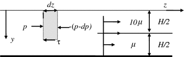

  

  Flow of two layered immiscible liquids

  • Determine the shear stress τ = τ(y), and in particular its value at the wall, τ _w  = τ(H).

  • Find the fluid velocity at the interface, v(H/2), and the velocity at the free surface, v(0).

  • Sketch qualitatively the velocity field.

• 7.3 A Newtonian fluid with viscosity μ flows in a canal of height H. Using the same Cartesian axes as in Fig. 7.9, assume that the air resistance at the free surface, y = 0, can be neglected, while at the wall, y = H, the fluid moves with a, so called, slip velocity., equal to v _w  = a|dv/dz| _w , where a is a characteristic length, e.g., the wall roughness. Find the velocity profile and, in particular, its maximum value.