
Abstract
After discussing the static electric field and steady currents, we are now ready to take another significant step in the study of electromagnetics, the study of the static magnetic field. But what exactly is a magnetic field? This question will be answered gradually, but, for a simple description, we may say it is a new type of force field in the same sense that the electric field is a force field. Take, for example, a magnet. It attracts or repels other magnets and generates a “magnetic field” around itself. The permanent magnet generates a static (time-independent) magnetic field. A direct current can also generate a static magnetic field. How do we know that? As with many other aspects of electromagnetics, we know by experiment.
“There’s a South Pole,” said Christopher Robin, “and I expect there’s an East Pole and a West Pole, though people don’t like talking about them.”
Winnie-The-Pooh
This is a preview of subscription content, log in via an institution.
Buying options
Tax calculation will be finalised at checkout
Purchases are for personal use only
Learn about institutional subscriptionsNotes
- 1.
Hans Christian Oersted (1777–1851), Danish scientist and professor of physics. He tried for many years to establish the link between electricity and magnetism, a link that was suspected to exist by him and many other scientists of the same period. He finally managed to do so in his now famous experiment of 1819 in which he showed that a current in a wire affects a magnetic needle (compass needle). He disclosed his experiments, all made in the presence of distinguished witnesses, in 1820. Oersted was very careful to ensure that what he saw was, in fact, a magnetic phenomenon by repeating the experiments many times and with various “needles,” in addition to the magnetic needle (to show that the effect does not exist in conducting materials such as copper or insulating materials such as glass—only in magnetized materials). Intervening materials between the wire and needle were also tested. As was the custom of the day, his work was written and communicated in Latin in a pamphlet titled: “Experimenta circa efficaciam, conflictus eletrici in acum magneticam.”
- 2.
See the footnote on page 341.
- 3.
Hendrik Antoon Lorentz (1853–1928). Dutch physicist who is best known for his work on the effects of magnetism on radiation. For this he received the Nobel Prize in 1902. In his attempt to explain electricity, magnetism, and light, he arrived at the Lorentz transformation, which helped Albert Einstein in formulating his theory of relativity.
- 4.
Jean-Baptiste Biot (1774–1862) was a professor of physics and astronomy. Among other topics, he worked on optics and the theory of light. Felix Savart (1791–1841) was a physician by training but later became professor of physics. This law is attributed to Biot and Savart because they were the first to present quantitative results for the force of a current on a magnet (in fact quantifying Oersted’s discovery). The experiments mentioned here are described in detail in James Clerk Maxwell’s Treatise on Electricity and Magnetism (Part IV, Chapter II), as Ampere’s experiments. The law was presented in 1820, about a year after the landmark experiment by Oersted established the link between current and the magnetic field.
- 5.
Ampere’s law is named after Marie Andre Ampere (see footnote on page 341). Ampere derived this law from study of the solenoidal (circular) nature of the magnetic field of straight wires.
- 6.
After Nicola Tesla (1856–1943). Tesla is well known for his invention of AC electric machines and development of the multiphase system of AC power. This happened in the early 1880s, followed by a number of other important engineering designs, including the installation of the first, large-scale AC power generation and distribution system at Niagara Falls (approx. 12 MW), in 1895. His induction motor became a staple of AC power systems, but his patents (about 500 in all) include transformers, generators, and systems for transmission of power. Tesla also had designs of grandiose scale, including “worldwide aerial transmission of power,” high-frequency, high-voltage generators and many others. Tesla was always somewhat of a “magician” and liked to keep his audience guessing, but later in his life, he became more of an eccentric and a recluse. Although some of his designs were more dreams than engineering, he is considered by many as the greatest inventor in electrical engineering. His statement regarding his student pay that there are “too many days after the first of the month” is even more familiar than his inventions, even to those that never heard it.
- 7.
The search for monopoles (single magnetic poles) is still continuing in basic physics research. No evidence of their existence has ever been found either on macroscopic or microscopic levels.
- 8.
The magnetic vector potential was considered by James Clerk Maxwell to be a fundamental quantity from which the magnetic flux density was derived. He called it the “Electrokinetic Momentum.” In fact, Maxwell used the scalar and vector potentials to define fields. The fields as we use them today were introduced as fundamental quantities by Oliver Heaviside and Heinrich Hertz. Oliver Heaviside, in particular, had some harsh words about potential functions. He considered the magnetic vector potential an “absurdity” and “Maxwell’s monster,” which should be “murdered.” Harsh words, but then Heaviside had harsh words for many people and topics. Although we use Heaviside’s form of electromagnetics in using field variables, we also make considerable use of potential functions. The guiding rule for us is simplicity and convenience.
Author information
Authors and Affiliations
Problems
Problems
8.1.1 The Biot–Savart Law
-
8.1
Magnetic Flux Density Due to Filamentary Currents. A current I [A] flows in a conductor shaped as an equilateral triangle (Figure 8.27 ). Calculate the magnetic flux density at the center of gravity of the triangle (where the three normals to the sides meet).
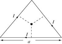
Figure 8.27
-
8.2
Flux Density of Current Segments. A conductor of length 2L [m] carries current I [A] and is bent as in Figure 8.28:
-
(a)
Calculate the magnetic flux density at point P.
-
(b)
Calculate the magnetic flux density at point O.
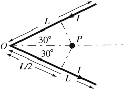
Figure 8.28
-
(a)
-
8.3
Application: Magnetic Field of Moving Charges. A thin insulating disk of outer radius b has a uniform charge density ρ s [C/m2] distributed over the surface between r = a [m] and r = b [m]. The charges are bound and cannot move from their location. If the disk is rotating at an angular velocity ω, calculate the magnetic field intensity at the center of the disk (Figure 8.29 ). Note. The first experiment to show the equivalency between moving charges and magnetic field was produced by Henry A. Rowland (1849–1901) in 1875. He showed that a charge placed on a disk (rotating at 3660 rpm) produced a magnetic field exactly like that of a closed-loop current.
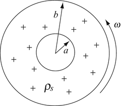
Figure 8.29
-
8.4
Magnetic Flux Density of Semi-infinite Segments. An infinitely long wire carrying a current I [A] is bent as shown in Figure 8.30. Find the magnetic flux density at points P 1 and P 2. (P 2 is at the center of the horizontal wire, at a distance d [m] from the bend.)
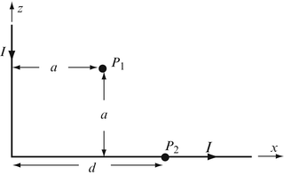
Figure 8.30
-
8.5
Magnetic Flux Density of a Loop. A square loop carries a current I [A]. Calculate the magnetic flux density (magnitude and direction) at a point h [m] high above the center of the loop (see Figure 8.31 ).
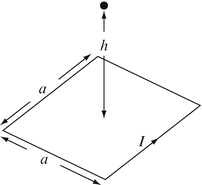
Figure 8.31
-
8.6
Magnetic Flux Density of a Spiral Coil. A wire is bent to form a flat spiral coil and carries a current I [A]. Calculate the flux density at a point h [m] high above the center of the spiral (Figure 8.32 ). The coil radius is a [m]. The spiral has N uniformly distributed turns. Assume each turn is a perfect circle.
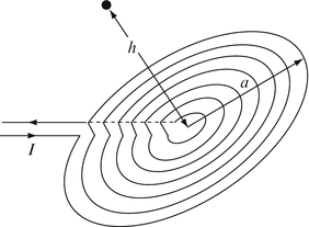
Figure 8.32
-
8.7
Magnetic Fields of Planar Structures. A semiconductor material is made as shown in Figure 8.33. The long ends of the piece are connected to a voltage source. This causes electrons to move toward the positive connection and holes toward the negative connection. Holes and electrons move at the same velocity v [m/s] and have the same charge magnitude q [C] each. The hole and electron densities are equal to ρ holes/m3 and ρ electrons/m3, respectively:
-
(a)
Set up the integrals needed to calculate the magnetic flux density at a height h [m] from the center of the piece (see Figure 8.33 ). Do not evaluate the integrals.
-
(b)
Optional: Evaluate the integrals in (a) for the following data: a = 0.02 m, b = 0.05 m, d = 0.5 m, h = 0.1 m, ρ = 1020 (holes or electrons/m3), v = 1 m/s, q = 1.6 × 10⁻¹⁹ C. Note. The integration is very tedious. You may wish to perform the integration numerically.
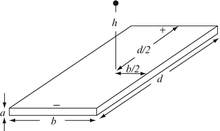
Figure 8.33
-
(a)


8.1.2 Ampere’s Law
-
8.8
Magnetic Flux Density of Thick Conductors. Two, infinitely long cylindrical conductors of radius a [m] carry a current I [A] each. One conductor coincides with the y axis, whereas the second is parallel to the z axis, in the x−z plane, at a distance d from the origin as shown in Figure 8.34. The currents are in the positive y direction in the first conductor and in the positive z direction in the second conductor. Calculate the magnetic flux density (magnitude and direction) at all points on the z axis.
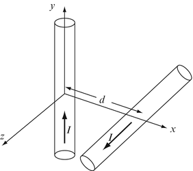
Figure 8.34
-
8.9
Magnetic Flux Density of Thick Conductors. Two infinitely long cylinders, one of radius a [m] and one of radius b [m], are separated as shown in Figure 8.35. One cylinder is directed parallel to the z axis, in the x−z plane, the other parallel to the y axis, in the x−y plane. A current density J [A/m2] flows in each, directed in the positive y and z directions as shown. Calculate the magnetic flux density at a general point P(x,y,z) outside the cylinders.
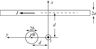
Figure 8.35
-
8.10
Application: Magnetic Flux Density Due to Power Lines. A high-voltage transmission line operates at 750 kV and 2000 A maximum. The towers used to support the lines are h = 20 m high and the lines are separated a distance 2a = 6 m (Figure 8.36 ). Calculate:
-
(a)
The magnetic flux density anywhere at ground level.
-
(b)
The magnetic flux density (magnitude and direction) at ground level, midway between the two wires.
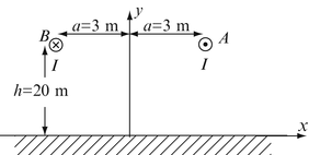
Figure 8.36
-
(a)


8.1.3 Ampere’s Law, Superposition
-
8.11
Magnetic Flux Density Due to Volume Distribution of Currents. A very long, L-shaped conductor with dimensions shown in cross section in Figure 8.37 carries a total current I [A]. The current is in the positive z direction (out of the paper) and is uniformly distributed in the cross-section:
-
(a)
Set up the integrals needed to calculate the magnetic flux density (magnitude and direction) at point P(a,a).
-
(b)
Optional: Evaluate the integrals in (a) for the following data: a = 0.05 m, b = 0.025 m, I = 100 A. Note. The integration is very tedious. You may wish to perform the integration numerically.
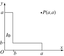
Figure 8.37
-
(a)
-
8.12
Magnetic Field of a Current Sheet. A thin layer of wires forms an infinite sheet of current. There are N wires per meter and each wire carries a current I [A] as shown in Figure 8.38. Calculate the magnitude and direction of the magnetic flux density everywhere in space.
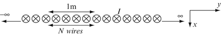
Figure 8.38
-
8.13
Application: Magnetic Field of Thin and Thick Conductors. An infinitely long thin wire is placed at the center of a hollow, infinitely long cylindrical conductor as shown in Figure 8.39. The conductor carries a current density J [A/m2] and the wire carries a current I [A]. The direction of J is out of the page. Find the magnetic flux density for the regions 0 < r < r1, r 1 < r < r 2, r > r 2 for the following conditions: (a) I = 0. (b) I in the direction of J. (c) I in the direction opposing J.
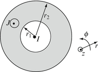
Figure 8.39
-
8.14
Magnetic Flux Density Due to Rotating Surface Charge Density. A long conducting cylinder of radius b [m] contains a surface charge density equal to ρ s [C/m2] on its outer surface. The cylinder spins at an angular velocity ω [rad/s] around its axis (Figure 8.40 ). Calculate the magnetic field intensity everywhere in space.
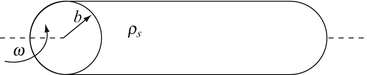
Figure 8.40
-
8.15
Superposition of Magnetic Flux Densities Due to Thick Conductors. A hollow, infinitely long cylindrical conductor has an outer radius b [m] and an inner radius a[m]. An offset cylinder of radius c [m] is located inside the large cylinder as shown in Figure 8.41. The two cylinders are parallel and their centers are offset by a distance d [m]. Assuming that the current density in each cylinder is J [A/m2] and is uniform, calculate the magnetic flux density at point A (outside the larger cylinder). The current in the larger cylinder is out of the page, and in the smaller cylinder, it is into the page.
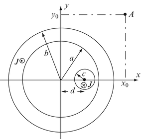
Figure 8.41
-
8.16
Application: Magnetic Field in a Coaxial Cable. Given a very long (infinite) wire with current I [A] and a very long (infinite) cylindrical tube of thickness r 2 – r 1 with uniform current density J 1 [A/m2] as shown in Figure 8.42, find:(a) B for 0 < r < r 1, (b) B for r 2 < r < ∞.
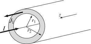
Figure 8.42
-
8.17
Magnetic Field in Coaxial Solenoids. A long solenoid (a single layer of very thin wires) of radius r 1 [m] is placed inside a second long solenoid of radius r 2 [m]. The currents in the solenoids are equal but in opposite directions, as shown in Figure 8.43a in axial cross section, and each solenoid has n turns per meter length:
-
(a)
Calculate the magnetic flux density for 0 < r < r 1, r 1 < r < r 2 and r > r 2.
-
(b)
Repeat (a), if the current in the inner solenoid is reversed.
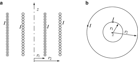
Figure 8.43
-
(a)
-
8.18
Superposition of Solutions in Solid Conductors. A very long (infinite) tubular conductor has radius b [m] and an offset hole of radius c as shown in Figure 8.44. The center of the hole is offset a distance d [m] from the center of the conductor. If the current density in the conductor flows out of the paper and equals J [A/m2], calculate the magnetic field intensity at A.
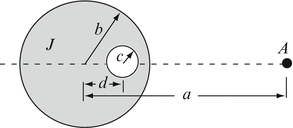
Figure 8.44
-
8.19
Fields Due to Current Sheets. Two infinite, thin sheets of current are arranged as shown in Figure 8.45. In the upper sheet, the current flows to the right, and in the lower, it flows out of the page. Calculate the magnetic field intensity everywhere. The current density is given in A/m meaning that the thickness of the sheets is negligible.
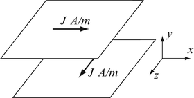
Figure 8.45


8.1.4 Biot–Savart Law, Magnetic Vector Potential
-
8.20
Magnetic Vector Potential of Current Segment. A very long (but not infinite) straight wire carries a current I [A] and is located in free space:
-
(a)
Calculate the magnetic vector potential at a distance a [m] from the center of the wire. Assume for simplicity that the wire extends from − L [m] to + L [m] and that L ≫ a.
-
(b)
From the result in (a), what must be the magnetic vector potential for an infinitely long current-carrying wire?
-
(a)
-
8.21
Magnetic Vector Potential of Loops. A circular loop and a square loop are given as shown in Figure 8.46:
-
(a)
Find the ratio between the magnetic flux densities at the center of the two loops.
-
(b)
What is the magnetic vector potential at the center of each loop? Hint. Use Cartesian rather than cylindrical coordinates for the integration for both loops.
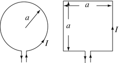
Figure 8.46
-
(a)
-
8.22
Application: Magnetic Flux. A straight wire carries a current I = 1 A. A square loop is placed flat in the plane of the wire as shown in Figure 8.47. Calculate:
-
(a)
The flux, using the magnetic flux density.
-
(b)
The flux, using the magnetic vector potential. (Hint. Use the result of Problem 8.20 . Compare the results in (a) and (b).)
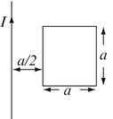
Figure 8.47
-
(a)
-
8.23
Magnetic Flux. A straight, infinitely long wire carries a current I = 10 A and passes above a loop of radius a = 0.1 m as shown in Figure 8.48a:
-
(a)
If the wire passes as in Figure 8.48a, show from symmetry considerations that the total flux through the loop is zero, regardless of how close the loop and the wire are.
-
(b)
If the loop is moved sideways as in Figure 8.48b, calculate the total flux through the loop. Assume the loop and wire are in the same plane.
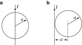
Figure 8.48
-
(a)


8.1.5 Magnetic Scalar Potential
-
8.24
Magnetic Scalar Potential Between the Poles of a Permanent Magnet. The magnetic flux density between the poles of a large magnet is 0.1 T and is uniform everywhere between the poles in Figure 8.49. Calculate the magnetic scalar potential difference between the poles.
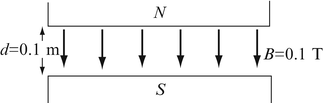
Figure 8.49
-
8.25
Magnetic Scalar Potential Between the Poles of a Permanent Magnet. The magnetic scalar potential difference between the poles of a magnet is 100 A (Figure 8.50 ). Calculate the magnetic field intensity if the space between the poles is air and the magnetic field intensity is uniform.
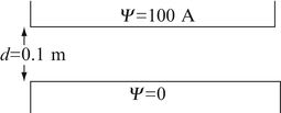
Figure 8.50


Rights and permissions
Copyright information
© 2015 Springer International Publishing Switzerland
About this chapter
Cite this chapter
Ida, N. (2015). The Static Magnetic Field. In: Engineering Electromagnetics. Springer, Cham. https://doi.org/10.1007/978-3-319-07806-9_8
Download citation
DOI: https://doi.org/10.1007/978-3-319-07806-9_8
Publisher Name: Springer, Cham
Print ISBN: 978-3-319-07805-2
Online ISBN: 978-3-319-07806-9
eBook Packages: EngineeringEngineering (R0)