Faraday’s Law and Induction

Abstract

In the previous chapters, we found it useful to treat the electric and magnetic phenomena separately. In Chaps. 4–7, we treated electrostatic fields by relying on the two postulates:

$$ \left(\nabla \times \mathbf{E}=0\kern0.6em \mathrm{and}\kern0.6em \nabla \cdot \mathbf{D}=\rho \right)\kern0.6em \mathrm{or}\kern0.6em \left({\displaystyle {\oint}_C\mathbf{E}\cdot d\mathbf{l}}=0\kern0.6em \mathrm{and}\kern0.6em {\displaystyle {\oint}_s\mathbf{D}\cdot d\mathbf{s}=Q}\right) $$

In Chaps. 8 and 9, some of the basic magnetic phenomena were introduced, now relying on the following two postulates:

$$ \left(\nabla \times \mathbf{H}=\mathbf{J}\kern0.6em \mathrm{and}\kern0.6em \nabla \cdot \mathbf{B}=0\right)\kern0.6em \mathrm{or}\kern0.6em \left({\displaystyle {\oint}_C\mathbf{E}\cdot d\mathbf{l}=I}\kern0.6em \mathrm{and}\kern0.6em {\displaystyle {\oint}_s\mathbf{B}\cdot d\mathbf{s}=0}\right) $$

These postulates allowed us to treat a large number of applications and gain insight into the behavior of the electric and magnetic fields governed by the postulates.

Whether Ampere’s beautiful theory were adopted, or any other, or whatever reservation were mentally made, still it appeared very extraordinary, that as every electric current was accompanied by a corresponding intensity of magnetic action at right angles to the current, good conductors of electricity, when placed within the sphere of this action, should not have any current induced through them, or some sensible effect produced equivalent in force to such a current.

—Michael Faraday (1791–1867), article 3 in the first series of

“Experimental Researches in Electricity,” Nov. 24, 1831

Problems

10.1.1 Motional emf

• 10.1 Motional emf. Two trains approach each other at velocities v ₁ and v ₂ as shown in Figure 10.37. Assume the trains’ axles are good conductors and the rails have a resistance r [Ω/km]. Use d = 2 m. The trains are P = 10 km apart. Also given: v ₁ = 100 km/h, v ₂ = 120 km/h, r = 0.1 Ω/km. The vertical component of the terrestrial magnetic flux density is B ₀ = 0.05 mT. Calculate:

  • (a) The current in the rails produced by the motion of the trains in the terrestrial magnetic flux density at the instant shown in Figure 10.37.

    

    Figure 10.37

  • (b) The current in the rails as a function of time taking t = 0 at the instance shown in Figure 10.37.

• 10.2 Application: Motional emf as a Motion Detector Mechanism. Suppose you want to know if a train is moving on a rail but it is too far to see. Assume the rails are a distance d [m] apart and are insulated from each other. To check for motion of the train, you measure the potential difference between the two rails:

  • (a) Calculate the velocity of the train assuming that the magnetic flux density of the Earth is equal to B ₀ [T] and is perpendicular to the surface of the Earth, pointing downward. The potential difference measured is V [V] with its positive pole on the top rail in Figure 10.38.

    

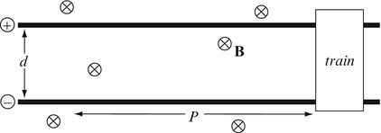
    Figure 10.38

  • (b) In which direction is the train moving?

  • (c) If the resistance per meter length of a rail equals r [Ω/m], calculate the distance P from the measurement point to the train. How can this distance be found by a simple measurement at the point where the observer is located?

  • (d) Can these measurements be used to avoid collision of trains?

10.1.2 Induced emf

• 10.3 Forces Due to Induction. Two very long, parallel rails are placed in a uniform, time-dependent magnetic field. The resistance of the rails is negligible. On the left side, the rails are shorted with a wire of resistance R [Ω]. The wire is fixed and not allowed to move. On the right, a bar with zero resistance is placed on the rails (Figure 10.39 ) so that it is free to move. The magnetic flux density is given as $\mathbf{B}=-\widehat{\mathbf{z}}{B}_0\kern-0.12em \cos \kern-0.15em \left(\omega t\right)$ [T]:

  • (a) Calculate the magnitude and direction of the force acting on this bar in the instance shown in Figure 10.39.

  • (b) What is the force at t = 0?

  • (c) Suppose now that the bar is free to move. Describe qualitatively the motion of the bar.

    

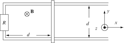
    Figure 10.39

• 10.4 Motional emf. An infinitely long, straight wire of radius r ₁ [m] carries a uniform current density J [A/m²]. The direction of the current is as shown in Figure 10.40. Another infinite, thin wire parallel to the first wire moves to the right at a velocity v ₀ [m/s]. Calculate the induced voltage (emf) per unit length in the moving wire, when the moving wire is at a distance r [m] from the thick wire. The wires are shown in cross-section.

  

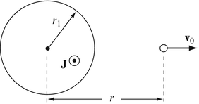
  Figure 10.40

• 10.5 Induced emf in a Plate. An infinitely long strip of conducting material of width d [m] moves in a uniform, sinusoidal magnetic flux density B = B ₀cosωt [T] at a constant velocity v [m/s]. The field makes a 45° angle with the direction of movement of the strip. Calculate the induced emf between any two points on opposite sides (a, b) of the strip (Figure 10.41 ). Show polarity.

  

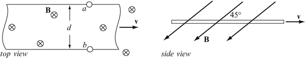
  Figure 10.41

• 10.6 Induced emf in a Rotating Bar. Two conducting hoops, each of radius r ₁ [m], are connected at one point by a straight conducting bar. The two hoops are kept parallel to each other and rotate at 600 rpm in a constant magnetic field as shown in Figure 10.42. The magnetic field is parallel to the hoops and perpendicular to the bar. Calculate the potential difference (emf) between the two hoops.

  

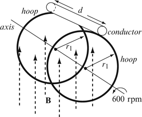
  Figure 10.42

• 10.7 Motion and Transformer Action emf in Loops. A square loop and a round loop move at a constant velocity v ₀ [m/s] in the x direction $\left(\mathbf{v}=\widehat{\mathbf{x}}{v}_0\right)$, as shown in Figure 10.43. The magnetic field intensity is given as $\mathbf{H}=\widehat{\mathbf{z}}{H}_0\kern-0.12em \cos \kern-0.15em \left(\omega t\right)$ [A/m]. Calculate the ratio between the induced voltages (emf) in the two loops.

  

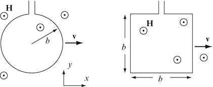
  Figure 10.43

• 10.8 Application: Generation of Very High emf/Current: Explosive Method. A long solenoid has a total of N turns of radius d. The solenoid is placed in the magnetic flux density of the Earth, B, such that B is parallel to its axis, and the two ends of the solenoid are shorted. The total resistance of the wires of the solenoid is R. Using an explosive charge, the solenoid is collapsed (i.e., it is flattened sideways as shown in Figure 10.44). Calculate the current generated in the solenoid (average) during the collapsing of the solenoid assuming that this happens in a time Δt. Use Δt = 1μs, B = 0.00005 T, N = 1,000, R = 1 Ω, d = 1 m. Note. Explosive methods are sometimes used to generate very high magnetic fields of short duration for research purposes. This problem looks at the emf and short circuit currents of the collapsing coil.

  

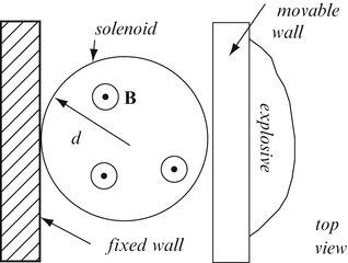
  Figure 10.44

10.1.3 Generator emf

• 10.9 emf in a Generator. A piece of wire is bent and rotated in a uniform, magnetic field B [T] as shown in Figure 10.45. The frequency of rotation is f (rotations per second). Calculate the induced emf between the terminals a and b. Show the polarity of the induced voltage (emf).

  

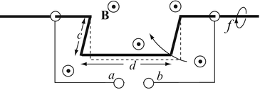
  Figure 10.45

• 10.10 emf in Rotating Bar. A conducting bar of length l [m] is pivoted at one end and rotates at an angular velocity ω [rad/s] in a magnetic field B [T] (z directed). Find the induced emf on the bar if it rotates perpendicular to the flux density in the counterclockwise direction for:

  • (a) $\mathbf{B}=\widehat{\mathbf{z}}{B}_0$.

  • (b) $\mathbf{B}=\widehat{\mathbf{z}}{B}_0{e}^{-r},\;0\le r\le l$.

• 10.11 Homopolar Generator. A spoked, conducting wheel rotates in an AC magnetic field as shown in Figure 10.46. The frequency of rotation is ω [rad/s]. The magnetic field intensity is H = 10⁶cos(ωt) [A/m]. A conducting hoop is provided on which the outer wire slides freely:

  • (a) Calculate the induced voltage (emf) between the center of the wheel and its outer perimeter.

  • (b) How does the solution change if the wheel is a solid conducting wheel?

  

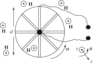
  Figure 10.46

• 10.12 Application: Homopolar Generator. A disk of radius 100 mm rotates in a uniform magnetic flux density at 6,000 rpm as shown in Figure 10.47. The magnetic flux density is sinusoidal, with amplitude 0.1 T and frequency 400 Hz. A wire is connected to the center of the disk and one is sliding on its edge, making good contact. Calculate the voltage (motional emf) between points A and B.

  

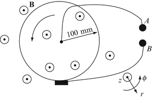
  Figure 10.47

• 10.13 Power Line Current Sensor. A sensor designed to detect and estimate the current in a power line remotely is proposed as follows: A small coil of area S is placed at ground level at the center between the two conductors of an AC power line (see Figure 10.48 ). The line carries a current I ₀ (RMS) at frequency f and is sinusoidal. The surface of the loop is parallel to the ground. If the height of the lines and their separation is known, find a relation between the current in the line and the emf produced in the coil. Assume the coil has area S [m²] and N turns. All materials involved have permeability of free space.

  

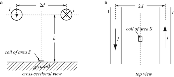
  Figure 10.48

• 10.14 Torque in Acyclic Motor. A disk of radius 100 mm is placed in a uniform DC magnetic flux density of 0.2 T. A wire is connected to the center of the disk, and one is sliding on its edge, making good contact. The disk is connected to a DC source that supplies a current of 100 A through the disk (Figure 10.49 ). Calculate the torque generated by the device.

  

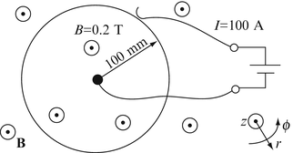
  Figure 10.49

10.1.4 Transformers

• 10.15 Ideal Transformer. An ideal transformer has a primary to secondary turn ratio of 10. If the transformer’s primary coil is connected to 110 V and transfers 150 W, calculate:

  • (a) The voltage and current in the secondary.

  • (b) The current in the primary.

  • (c) The impedance of the primary and secondary coils. What is the ratio between the impedance in the primary and secondary?

• 10.16 Current Transformer. An infinitely long, thin wire, carrying a current I, is located at the center of a torus as shown in Figure 10.50. Calculate the induced voltage (emf) in an N turn coil, uniformly distributed around the torus. Use a = 20 mm, b = 30 mm, d = 10 mm, f = 100 Hz, I ₀ = 1 A, μ _r = 100, μ ₀ = 4π × 10⁻⁷ H/m, N = 200.

  

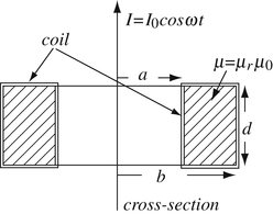
  Figure 10.50

• 10.17 Application: High-Power Ideal Transformer. A transformer is used in a hydroelectric power plant to step up the output from a 720 MW generator. The generator operates at 60 Hz, 18 kV. The output voltage required for transmission is 750 kV:

  • (a) If an ideal transformer is used, calculate the turn ratio and input and output currents at full load.

  • (b) Ideal transformers do not exist. Suppose the transformer has 1 % losses (typical for these transformers). Calculate the required turn ratio to maintain an output voltage of 750 kV at full load. Assume all power loss occurs in the iron core of the transformer.

  • (c) Calculate the output current and the flux in the magnetic core for rated input power with the turn ratio in (b). Use a relative permeability of 1,000, length of the magnetic path of 4 m, and cross-sectional area of 0.2 m². Assume that the number of turns in the primary is given as N ₁ = 10.

• 10.18 Application: Design of a Current Transformer. You have an AC digital voltmeter with its basic range 199.9 mV rms and are requested to monitor the input power to a house by measuring the input current. The maximum current expected is 150 A (rms) at 60 Hz. You choose to build a simple current transformer by cutting an iron ring (so that the ring can be slipped over the wire) and winding a coil on the ring. The emf in this coil is your reading. The ring is of average radius of 20 mm, a cross-sectional area of 100 mm², and relative permeability of 200:

  • (a) How many turns are required to produce full-scale reading for maximum input?

  • (b) Suppose you wish now to use the same device to measure currents up to 500 A (rms). How many turns are required for this purpose?

• 10.19 Application: Transformer with Multiple Windings. The magnetic circuit in Figure 10.51 is given. Coil 1 has N ₁ = 100 turns and carries a current I ₁ = I ₀cos(ωt) and coil 2 has N ₂ = 50 turns and carries a current I ₂ = I ₀cos(ωt) where I ₀ = 1 A, ω = 314 rad/s. The currents in the two coils are such that the magnetic flux density is in the direction shown in the figure. Coil 3 has N ₃ = 1,000 turns. Dimensions are average lengths and are given in the figure. The cross-sectional area of the core is 100 cm². Relative permeability of the core is 100:

  • (a) Calculate V ₁ and V ₂ (the voltages across the terminals of coils No. 1 and No. 2).

  • (b) Calculate the induced voltage in coil No. 3.

  

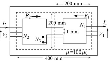
  Figure 10.51

• 10.20 Application: Loosely Coupled Transformer. Two coils, each with inductance of 10 mH, are placed next to each other to form a transformer. It was determined that the coefficient of coupling between the coils is 0.1 (i.e., 10 % of the flux produced by each coil passes through the second coil). One coil, designated as the primary, is connected to a sinusoidal current with amplitude 1 A and frequency of 100 kHz. Calculate:

  • (a) The emf in the primary and secondary with the secondary open circuited.

  • (b) The emf in the primary and secondary if a current of amplitude 0.05 A is drawn from the secondary.

• 10.21 Induced Current in a Loop: A Nonconventional Transformer. Determine the induced voltage (emf) v(t) in the rectangular loop shown next to a very long wire carrying a time-varying current I(t) = I ₀sinωt [A] (Figure 10.52).

  

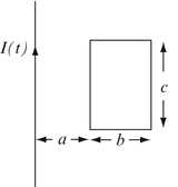
  Figure 10.52

• 10.22 Current Transformer with Air Core. Calculate the induced voltage (emf) in an air-filled, uniformly wound toroidal coil of N turns and cross-sectional area as shown in Figure 10.53. The central wire is very long and carries a current I(t) = I ₀sinωt [A].

  

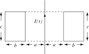
  Figure 10.53

• 10.23 Application: Power Line Power Scavenging for Sensing. As part of a smart grid, one proposes to place sensors on power lines to sense a variety of parameters such as temperature, current, corrosion, vibrations, and others and transmit these parameters wirelessly to a central location. To do so, the sensors are placed on the power line itself by attaching them to one conductor of the power line. To power the sensors and the wireless transmitter, one can use the magnetic field produced by the line by designing an appropriate transformer. A solution is to place a toroidal coil around the conductor as shown in Figure 10.54. Suppose a power line carries a sinusoidal current I = 500 A (RMS) at a frequency f = 60 Hz. The toroidal core has an inner radius a = 30 mm, outer radius b = 50 mm, and thickness c = 20 mm. Its relative permeability is 100:

  • (a) Calculate the number of turns needed on the torus to produce an RMS voltage of 6 V.

  • (b) What is the maximum theoretical power available for use in the sensors?

    Figure 10.54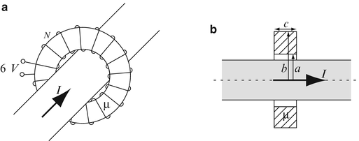

    

    Structure of power line power scavenging. (a) General view, (b) axial cross section

• 10.24 Ground Fault Circuit Interrupt (GFCI). An important safety device is the GFCI (also called a residual current device (RCD)). It is intended to disconnect electrical power if current flows outside of the intended circuit, usually to ground, such as in the case when a person is electrocuted. The schematic in Figure 10.55 shows the concept. The two conductors supplying power to an electrical socket or an appliance pass through the center of a toroidal coil. Normally the currents in the two conductors are the same and the net induced emf due to the two conductors cancel each other, producing a net zero output in the current sensor. If there is a fault and current flows to ground, say a current I _g , the return wire will carry a smaller current and the current sensor produces an output proportional to the ground current I _g . If that current exceeds a set value (typically 30 mA), the induced emf causes the circuit to disconnect. These devices are common in many locations and are required by code in any location in close proximity to water (bathrooms, kitchens, etc.).

  Figure 10.55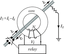

  

  Principle of a GFCI sensor

  Consider the GFCI shown schematically in Figure 10.55. The device is designed to operate in a 50 Hz installation and trip when the output voltage is 100 μV RMS. For a toroidal coil with average diameter a = 30 mm and a cross-sectional diameter of b = 10 mm:

  • (a) Calculate the number of turns needed if an air-filled toroidal coil is used and the device must trip at a ground current of 6 mA.

  • (b) Calculate the number of turns needed to trip at a current of 6 mA if a ferromagnetic torus with relative permeability of 2,000 is used as a core for the coil.

• 10.25 Application: The MHD Generator. A small magnetohydrodynamic (MHD) generator is proposed as part of the exhaust system of a jet engine. The MHD channel is 200 mm by 200 mm in cross section and is 1 m long. A magnetic field of 1 T is generated between two surfaces as shown in Figure 10.56. The exhaust moves at 200 m/s and is seeded to produce a conductivity of 50 S/m in the channel. Calculate:

  

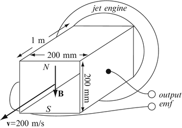
  Figure 10.56

  • (a) The output voltage (emf) of the generator. Show polarity.

  • (b) The internal resistance of the generator.

  • (c) Maximum power output to a load under maximum power conditions.