Mechanical System Lifetime

Abstract

We present, in three parts, the approaches for the random loading analysis in order to complete methods of lifetime calculation.

First part is about the analysis methods. Second part considers modeling of random loadings. A loading, or the combination of several loadings, is known as the leading cause of the dwindling of the mechanical component strength. Third part will deal with the methods taking into account the consequences of a random loading on lifetime of a mechanical component.

The motivations of the present document are based on the observation that operating too many simplifications on a random loading lost much of its content and, therefore, may lose the right information from the actual conditions of use. The analysis of a random loading occurs in several ways and in several approaches, with the aim of later evaluate the uncertain nature of the lifetime of a mechanical component.

Statistical analysis and frequency analysis are two complementary approaches. Statistical analyses have the advantage of leading to probabilistic models (Demoulin B (1990a) Processus aléatoires [R 210]. Base documentaire « Mesures. Généralités ». (*)) provide opportunities for modeling the natural dispersion of studied loadings and their consequences (cracking, fatigue, damage, lifetime, etc.). The disadvantage of these statistical analyses is that they ignore the history of events.

On the other hand, the frequency analyses try to remedy this drawback, using connections between, firstly, the frequencies contained in the loading under consideration and, secondly, whether the measured average amplitudes (studied with the Fourier transform, FT) or their dispersions (studied with the power spectral density, PSD) (Kunt M (1981) Traitement numérique des signaux. Éditions Dunod; Demoulin B (1990b) Fonctions aléatoires [R 220]. Base documentaire « Mesures. Généralités ». (*)). The disadvantage of frequency analyses is the need to issue a lot of assumptions and simplifications for use in models of lifetime calculation (e.g., limited to a system with one degree of freedom using probabilistic models simplified for the envelope of the loading).

A combination of the two analyses is possible and allows a good fit between the two approaches. This combination requires a visual interpretation of the appearance frequency. Thus, a random loading is considered a random process to be studied at the level of the amplitude of the signal, its speed, and its acceleration.

Appendices

Appendix 1: Main Solutions of the Pearson System and Replacement Laws

1.1 Introduction of the Bêta 1 Law

This law takes into account all possible asymmetries between 0 and 1.8. Regarding kurtosis, it takes into account the kurtosis between 1 and at most 5.8. This physically means that this law is limited in its horizontal extension. In fact, this law is theoretically defined on an interval. The standard form of the probability distribution is expressed as follows:

$$ {f}_X(x)=\frac{\gamma \left( p+ q\right)}{\gamma (p)\gamma (q)}{x}^{p-1}{\left(1- x\right)}^{q-1} $$

(28)

with: x between 0 and 1, $\gamma (t)={\displaystyle \underset{0}{\overset{\infty }{\int }}{\mathrm{e}}^{- u}{u}^{t-1}\; du}$, p and q are the shape parameters of the probability distribution. They are expressed in terms of the mean (m _X ) and standard deviation (s _X ) of the random variable X.

$$ p=-{m}_x+\frac{1-{m}_x}{{v_x}^2} $$

(29)

$$ q=\frac{m_x-1}{m_x}.\left({m}_x+\frac{m_x-1}{{v_x}^2}\right) $$

with v _x  = s _x /m _x coefficient of variation.

For a random variable which is defined between any two terminals (a and b), X is obtained by the following change of variable:

$$ X=\left( Y- a\right)/\left( b- a\right)$$

Thus, m _X  = (m _Y  − a)/(b − a) and s _X  = s _Y /(b − a).

Figure 22 shows different shapes of the probability law in function of p and q. This type of probability distribution is used for random stress that is physically defined between two terminals. Both terminals must be of the same order of magnitude.

Fig. 22

Probability density function f _x (x) of the Beta 1 law as a function of its parameters

1.2 Introduction of the Bêta 2 Law

This probability law takes into account the medium and high kurtosis. It also takes into account all possible asymmetries between 0 and 1.8. For these reasons, the law favors Beta 2 promotes kurtosis versus asymmetry. This law is theoretically defined from a low left δ (named offset) and infinity. It is easier to work with the “standard form” of this law. The “standard form” for a probability law which the variable varies between a threshold and infinity is obtained by a change of variable which leads to work with a probability density function which the variable varies between 0 (instead of δ) and infinity. The standard form of the probability distribution is expressed as follows:

$$ {f}_X(x)=\frac{\gamma \left( p+ q\right)}{\gamma (p)\gamma (q)}\frac{x^{p-1\ }}{{\left( x+1\right)}^{p+ q}} $$

(30)

with: x is between 0 and ∞.

p and q are the shape parameters of the probability distribution. They are expressed in terms of the mean (m _X ) and standard deviation (s _X ) of the random variable X.

$$ p={m}_x+\frac{m_x+1}{{v_x}^2} $$

and

$$ q=2+\frac{m_x+1}{m_x.{v_x}^2} $$

(31)

with v _x  = s _x /m _x .

Figure 23 shows various shapes of the probability law in function of p and q. For this chart, p is 3 and q is between 1 and 6. The variation of p leads only to homotheties on the curves of probability density. This kind of probability distribution is used for random stress which we observe (or we think) that physically dispersion phenomena or kurtosis are more predominant than the phenomena of asymmetry.

Fig. 23

Probability density function f _X (x) of the Beta 2 law as a function of its parameters

In the event that difficulties are encountered when handling this probability law, then it can be replaced by a Log-Normal law which is easier to operate. The standard form of the probability distribution is expressed as follows:

$$ {f}_X(x)=\frac{1}{\sigma \sqrt{2\pi}}\frac{1}{x}. \exp \left(-\frac{1}{2}{\left(\frac{ \ln (x)- m}{\sigma}\right)}^2\right) $$

(32)

with: x is between 0 and ∞.

$$ m= \ln \left(\frac{m_x}{\sqrt{1+{v_x}^2}}\right)\kern1em \mathrm{and}\kern1em \sigma =\sqrt{ \ln \left(1+{v_x}^2\right)} $$

(33)

For a random variable which is set between the infinite and δ, X is obtained by the following change of variables: X = (Y − δ). Thus, m _X  = (m _Y  − δ) and s _X  = s _Y . Figure 24 shows the good approximation of the Beta 2 law by Log-Normal law.

Fig. 24

Comparison between Beta 2 law and Log-Normal

1.3 Introduction of the Gamma law

According to the abacus of Pearson, the probability distribution is defined in the intermediate zone between Beta 1 law and Beta 2 law. Thus, its contribution is located mainly in consideration of asymmetry and less kurtosis. For this reason, the Gamma law promotes asymmetry versus kurtosis. This law is theoretically defined between a threshold δ and infinity. The standard form of the probability distribution is expressed as follows:

$$ {f}_X(x)=\frac{a^p}{\gamma (p)}{x}^{p-1}. \exp \left(- ax\right) $$

(34)

with: x is between 0 and ∞.

p and q are the shape parameters of the probability distribution. They are expressed in terms of the mean (m _X ) and standard deviation (s _X ) of the random variable X.

$$ p=\frac{1}{{v_x}^2}\kern1em \mathrm{and}\kern1em a=\frac{1}{m_x.{v_x}^2} $$

(35)

with v _x  = s _x /m _x .

Figure 25 shows different forms of the probability law function of a and p. For this graph, a is set to 1 and p is between 0.5 and 5. Variation of a led only to homotheties on the probability density curves. This kind of probability law is used for random stress which is observed (or is thought) that physically, the important phenomena of displacement of the medium or of asymmetry that are more predominant kurtosis phenomena.

Fig. 25

Probability density function f _x (x) of the Gamma distribution as a function of its parameters

As for the Beta 2 law, the gamma distribution can be replaced by another law easier to handle and well known is the Weibull distribution. The standard form of this law is expressed as follows:

$$ {f}_X(x)=\frac{\beta}{\eta}{\left(\frac{x}{\eta}\right)}^{\beta -1} \exp \left\{-{\left(\frac{x}{\eta}\right)}^{\beta}\right\} $$

(36)

with: x is between 0 and ∞.

With the expectation (or mean) and standard deviation, which are expressed as follows:

$$ E\left\{ X\right\}={m}_X=\eta \gamma \left(1+\frac{1}{\beta}\right) $$

and

$$ {s}_X=\eta \sqrt{\gamma \left(1+\frac{2}{\beta}\right)-{\left(\gamma \left(1+\frac{1}{\beta}\right)\right)}^2} $$

(37)

The β factor is often called form factor η and the scale factor. For a random variable which is set between the infinite and δ, X is obtained by the following change of variable:

$$ X=\left( Y-\delta \right).\kern0.5em \mathrm{Thus}\kern0.5em {m}_X=\left({m}_Y-\delta \right)\kern1em \mathrm{and}\kern1em {s}_X={s}_Y. $$

Figure 26 shows the good approximation of Gamma law with a WEIBULL law. Thus, WEIBULL law is the most appropriate model for modeling the random dispersion of mechanical stresses that are defined from a given threshold and that their asymmetry and kurtosis them put in the intermediate zone between the law of the Beta 1 and the Beta 2. In addition, WEIBULL law is easy to handle and estimation of its parameters methods is now well known.

Fig. 26

Comparison between Gamma law and WEILBULL law

Appendix 2: Method of Estimate of the Weibull Law Parameters Around the Four Types of Local Events

The separation of the four types of local events in four samples used to calculate indicators for each sample form: $\mathrm{mean}=\overline{x}$, standard deviation = s _X , asymmetry = G ₁ (or β ₁), and kurtosis = G ₂ or (β ₂). X, a random variable with Weibull W (β, η; δ = 0). The formulation of the probability density function of X, expectation (or its average) and standard deviation are given by the relations Eq. (37) of “Introduction of the Gamma law” of Annex A. Table below gives the theoretical expressions of the dispersion coefficient (v _X ), of the asymmetry G ₁ and of the kurtosis G ₂ the Weibull distribution. These formulas are expressed exclusively in terms of the form factor of the distribution (β).

$$ {v}_x=\frac{s_x}{m_x}=\frac{{\left({\gamma}_2-{\left({\gamma}_1\right)}^2\right)}^{1/2}}{\left({\gamma}_1\right)} $$

$$ {G}_1=\frac{\gamma_3-3{\gamma}_2{\gamma}_1+2{\left({\gamma}_1\right)}^3}{{\left({\gamma}_2-{\left({\gamma}_1\right)}^2\right)}^{3/2}} $$

$$ {G}_2=\frac{\gamma_4-3{\gamma}_3{\gamma}_1-3{\left({\gamma}_2\right)}^2+12{\gamma}_2{\left({\gamma}_1\right)}^2-6{\left({\gamma}_1\right)}^4}{{\left({\gamma}_2-{\left({\gamma}_1\right)}^2\right)}^2} $$

(38)

with ${\gamma}_r=\gamma \left(1+\frac{r}{\beta}\right)$ _.

Thus, the shape factor may be obtained β by inverting one of three functions v _x , G ₁, or G ₂. Figure 27 shows the theoretical evolution of v _x , G ₁, and G ₂. According to β which the v _X  = F ₁(β), G ₁ = F ₂(β), and G ₂ = F ₃(β). Given the shape of the last three functions, the easiest way is to reverse (a numerical method) function G ₁. Figure 28 shows a random stress representing the couple in an industrial vehicle stabilizer bar when passing over a poorly maintained road. The recording time is 5 min.

Fig. 27

Evolution of v _X , G ₁ and G ₂ of the law the Weibull based on shape factor parameters β

Fig. 28

Viewing the input torque to the front stabilizer bar of a motor vehicle

Table 4 presents the values obtained for the different parameters of Weibull laws for the four types of local events. Figure 29 shows the adequacy of the proposed relationship with histograms experimentally observed laws.

Table 4 Parameters of Weibull laws

Fig. 29

Histograms peaks > 0 and hollow < 0 and probability distributions of four local events

Appendix 3: Extrem Response Spectrum for a Random Loading

Extrem response ER is calculated from the maximum met once during the excitation time response. For recording a duration T, the total number of peaks above z0 is given by

$$ N={N}_{\mathrm{e}} T{F}_M\left({u}_0\right) $$

(39)

With F _M (u) = cumulative probability function given in E3 of Annex E and N _e is the number of extreme values.

The largest peak for the duration T (on average) approximately corresponds to u ₀ level that is exceeded only once, hence:

$$ {F}_M\left({u}_0\right)=1/\left({N}_{\mathrm{e}} T\right) $$

(40)

The level u ₀ is determined by successive iterations. Distribution F _M (u) is a decreasing function of u. We consider two values u, such that:

$$ {F}_M\left({u}_1\right)<{F}_M\left({u}_0\right)<{F}_M\left({u}_2\right) $$

(41)

and, at each iteration, the interval is reduced (u ₁, u ₂) until, for example:

$$ \frac{F_M\left({u}_1\right)-{F}_M\left({u}_2\right)}{F_M\left({u}_0\right)}\prec {10}^{-2} $$

(42)

Hence extrapolation:

$$ {z}_m\approx {z}_0={\left( V(X)\right)}^{1/2}\left\{\left[{u}_2-{u}_1\right]\frac{F_M\left({u}_1\right)-{F}_M\left({u}_2\right)}{F_M\left({u}_0\right)}+{u}_1\right\} $$

(43)

and ER = (2πf ₀)² Z _m .

With the same assumptions, the average number of threshold exceedances z = α response with positive slope during a recording period T for stress a Gaussian is given by the relationship:

$$ {N}_{\alpha}^{+}= T{N}_{\alpha}= T{N}_0 \exp \left(-\frac{\alpha \mathit{^2}}{2\sqrt{V(X)}}\right)\kern1em \mathrm{and}\kern1em {N}_0=\frac{1}{\pi}\sqrt{\frac{V\left({x}^{\prime}\right)}{V(x)}} $$

(44)

Considering that the threshold α is exceeded only once, is obtained by N ⁺ _α  = 1

$$ \alpha =\sqrt{2 V(X) \ln \left({N}_0 T\right)} $$

Whence

$$ \mathrm{ER}=4\pi \mathit{^2}{f}_0^2\sqrt{2 V(X) \ln \left({N}_0 T\right)} $$

(45)

In the case of a random stress whose PSD is represented by several levels (G _i  = Φ cf. Sect. 1) each of which is defined between two frequencies f _i et f _i+1, the various components of ER are obtained as follows:

$$ V(X)={\displaystyle \underset{0}{\overset{\infty }{\int }} G(f). df=\frac{1}{{\left(2\pi \right)}^4.{f}_0^3}\frac{\pi}{4.\xi}}{\displaystyle \sum_i{G}_i.\left[{I}_0\left({h}_i+1\right)-{I}_0\left({h}_i\right)\right]}$$

(46)

$$ V\left(\dot{X}\right)={\left(2\pi \right)}^2.{\displaystyle \underset{0}{\overset{\infty }{\int }}{f}^2. G(f). df=\frac{1}{{\left(2\pi \right)}^2.{f}_0}\frac{\pi}{4.\xi}}{\displaystyle \sum_i{G}_i.\left[{I}_2\left({h}_i+1\right)-{I}_2\left({h}_i\right)\right]}$$

(47)

$$ V\left(\ddot{X}\right)={\left(2\pi \right)}^4.{\displaystyle \underset{0}{\overset{\infty }{\int }}{f}^4. G(f). df={f}_0.\frac{\pi}{4.\xi}}{\displaystyle \sum_i{G}_i.\left[{I}_4\left({h}_i+1\right)-{I}_4\left({h}_i\right)\right]} $$

(48)

with $G(f)=\left| H(f)\right|{}^2.{G}_{\ddot{x}}(f)$, h _i  = f _i /f ₀ and h _i+1 = f _i+1/f _0.

$$ {I}_0=\frac{\xi}{\pi.\alpha}. \ln \left(\frac{h^2+\alpha h+1}{h^2-\alpha h+1}\right)+\frac{1}{\pi}.\left[\mathrm{Arctan}\left(\frac{2. h+\alpha}{2.\xi}\right)+\mathrm{Arctan}\left(\frac{2. h-\alpha}{2.\xi}\right)\right] $$

(49)

$$ {I}_2=-\frac{\xi}{\pi.\alpha}. \ln \left(\frac{h^2+\alpha h+1}{h^2-\alpha h+1}\right)+\frac{1}{\pi}.\left[\mathrm{Arctan}\left(\frac{2. h+\alpha}{2.\xi}\right)+\mathrm{Arctan}\left(\frac{2. h-\alpha}{2.\xi}\right)\right] $$

(50)

$$ {I}_4=\frac{4.\xi}{\pi}. h+\beta.{I}_2-{I}_0 $$

(51)

$$ \alpha =2.\sqrt{1-\xi \mathit{^2}};\kern1em \beta =2\left(1-2.\xi \mathit{^2}\right);\kern1em Q=1/\left(2.\xi \right) $$

(52)

with ξ = damping factor

Thus:

$$ {N}_{\mathrm{e}}=\frac{1}{\pi}\sqrt{\frac{V\left({x}^{{\prime\prime}}\right)}{V\left({x}^{\prime}\right)}},\kern1em {N}_0=\frac{1}{\pi}\sqrt{\frac{V\left({x}^{\prime}\right)}{V(x)}}\kern1em \mathrm{and}\kern1em I=\frac{N_0}{N_{\mathrm{e}}} $$

(53)

In cases where the statistical distribution of peaks (trough respectively) is modeled by a Weibull law W(β, η, δ) with β: shape factor, η; scale parameter and δ: shift (often close to zero), we seeks probability π _M (u ₀) exceeds a maximum for any level u ₀ of the amplitude of the response. π _M (u ₀) = 1 − F _M (u ₀) with:

$$ {F}_M\left({U}_0\right)={\displaystyle \underset{-\infty }{\overset{u_0}{\int }} p(u)\; du} $$

and over a period of observation T, the mean number of peaks is greater than u ₀ always N = n ⁺ _p . Tπ(u ₀). When N = 1, the corresponding level is defined by π(u ₀) = 1/(n ⁺ _p . T).

with

$$ \pi \left({u}_0\right)= \exp \left(-{\left(\frac{u_{{}_0}}{\eta}\right)}^{\beta}\right) $$

and knowing the value of n ⁺ _p , it has

$$ {u}_0=\eta.{\left[ \ln \left(\frac{{\ddot{Z}}_{\mathrm{eff}}. T}{2\pi.{\dot{Z}}_{\mathrm{eff}}}\right)\right]}^{1/\beta} $$

(54)

While the extrem response becomes

$$ \mathrm{ER}={\left(2\pi.{f}_0\right)}^2.\eta.{\left[ \ln \left(\frac{{\ddot{Z}}_{\mathrm{eff}}. T}{2\pi.{\dot{Z}}_{\mathrm{eff}}}\right)\right]}^{1/\beta} $$

(55)

Appendix 4: Theoretical Modeling of the Overrun of Level for a Gaussian Loading

In the Gaussian case, x(t), x′(t), and x ^″(t) are Gaussian random variables with three densities as successive probabilities:

$$ {g}_x(u)=\frac{1}{\sqrt{2\pi V(x)}}. \exp \left\{-\frac{u^2}{2 V(x)}\right\} $$

(56)

$$ {g}_{x^{\prime }}(v)=\frac{1}{\sqrt{2\pi V\left({x}^{\prime}\right)}}. \exp \left\{-\frac{v^2}{2 V\left({x}^{\prime}\right)}\right\} $$

(57)

$$ {g}_{x^{{\prime\prime} }}(w)=\frac{1}{\sqrt{2\pi V\left({x}^{{\prime\prime}}\right)}}. \exp \left\{-\frac{w^2}{2 V\left({x}^{{\prime\prime}}\right)}\right\} $$

(58)

Thus, we have:

$$ E\left\{\left|{x}^{\prime}\right|\right\}={\displaystyle \underset{-\infty }{\overset{+\infty }{\int }}\left| v\right|{g}_{x^{\prime }}(v)\; dv}=\sqrt{\frac{2}{\pi} V\left({x}^{\prime}\right)}$$

(59)

$$ E\left\{\left|{x}^{{\prime\prime}}\right|\right\}={\displaystyle \underset{-\infty }{\overset{+\infty }{\int }}\left| w\right|}{g}_{x^{{\prime\prime} }}(w)\; dw=\sqrt{\frac{2}{\pi} V\left({x}^{{\prime\prime}}\right)} $$

(60)

Thus, in the case of a Gaussian process, Eqs. (19), (20), and (21) can be written

$$ {N}_{\alpha}=\frac{1}{\pi}\sqrt{\frac{V\left({x}^{\prime}\right)}{V(x)}}. \exp \left\{-\frac{1}{2}\frac{\alpha^2}{V(x)}\right\} $$

(61)

$$ {N}_0=\frac{1}{\pi}\sqrt{\frac{V\left({x}^{\prime}\right)}{V(x)}} $$

(62)

$$ {N}_{\mathrm{e}}=\frac{1}{\pi}\sqrt{\frac{V\left({x}^{{\prime\prime}}\right)}{V\left({x}^{\prime}\right)}} $$

(63)

Hence expression of Gaussian irregularity factor

$$ {I}_{\mathrm{g}}=\frac{N_0}{N_{\mathrm{e}}}=\frac{V\left({x}^{\prime}\right)}{\sqrt{V(x) V\left({x}^{{\prime\prime}}\right)}} $$

(64)

From this factor, the factor ε is defined as the bandwidth of the studied process. The last (as I and I _g) is between 0 and 1.

Bandwidth is expressed by the number of zero crossings by increasing values N ₀ and the number of local maxima N _e (positive or negative) of the observation time. We put:

$$ \varepsilon =\sqrt{1-{I}_{\mathrm{g}}^2} $$

(65)

Notes:

• 1. The relation Eq. (65) is a definition and simply reflects the fact that, when a process narrowband N ₀ = N _e (see Fig. 11a) and therefore ε = 0, and when a broadband process (Fig. 11b) N _e > N ₀, where N _e ≫ N ₀ ε → 1.

• 2. When ε = 0, in the case of a trajectory narrowband cycle thinking has a precise meaning, since N ₀ = N _e.

• 3. When ε = 1, the notion of cycle is likely to various interpretations, the definition of “number of cycles” depends on the counting method.

Appendix 5: Envelope Modeling for a Gaussian Loading

For a Gaussian trajectory, correlation coefficient between the signal x(t) and its first derivative x′(t) is zero. As follows:

$$ {g}_{X{X}^{\prime }{X}^{{\prime\prime} }}\left( u, v, w\right)={g}_{X^{\prime }}(v)\ {g}_{X{X}^{{\prime\prime} }}\left( u, w\right) $$

Dual distribution ${g}_{x{ x}^{{\prime\prime} }}\left( u, w\right)$ between the signal and its second derivative is expressed in a bi-normal distribution:

$$ {g}_{x{ x}^{{\prime\prime} }}\left( u, w\right)=\frac{1}{2\pi \sqrt{k}} \exp \left[-\frac{1}{2 k}\left\{ V\left({x}^{{\prime\prime}}\right){u}^2+2 V\left({x}^{\prime}\right) uw+ V(x){w}^2\right\}\right] $$

(66)

with k = V(x)V(x ^″) − [V(x′)]²

The probability density peaks (Eq. (26)) to be written:

$$ \begin{array}{c}{f}_M\left(\alpha \right)=\mathrm{Prob}\left(\alpha <\mathrm{Max}\le \alpha + d\alpha \right)=\\ {}=\frac{\sqrt{1-{I}_{\mathrm{g}}^2}}{\sqrt{2\pi}}. \exp \left(-\frac{u^2}{2\left(1-{I}_{\mathrm{g}}^2\right)}\right)+\frac{I_{\mathrm{g}} u}{2} \exp \left(-\frac{u^2}{2}\right)\left[1+\mathrm{erf}\left(\frac{I_{\mathrm{g}} u}{\sqrt{2\left(1-{I}_{\mathrm{g}}^2\right)}}\right)\right]\end{array} $$

(67)

And the cumulative probability function is:

$$ \begin{array}{c}{F}_M\left(\alpha \right)=\mathrm{Prob}\left(\mathrm{Max}\le \alpha \right)\\ {}=\frac{1}{2}\left\{1-\mathrm{erf}\left(\frac{u}{\sqrt{2\left(1-{I}_{\mathrm{g}}^2\right)}}\right)\right\}+\frac{I_{\mathrm{g}}}{2} \exp \left(-\frac{u^2}{2}\right)\left\{1+\mathrm{erf}\left(\frac{I_{\mathrm{g}} u}{\sqrt{2\left(1-{I}_{\mathrm{g}}^2\right)}}\right)\right\}\end{array} $$

(68)

with ${I}_{\mathrm{g}}=\frac{V\left({X}^{\prime}\right)}{\sqrt{V(X) V\left({X}^{{\prime\prime}}\right)}}$ Gaussian irregularity factor,

$$ u=\frac{\alpha}{\sqrt{V(X)}}\kern1em \mathrm{and}\kern1em \mathrm{erf}(x)=\frac{2}{\sqrt{\pi}}{\displaystyle \underset{0}{\overset{x}{\int }}{\mathrm{e}}^{-{\lambda}^2/2}\; d\lambda}. $$

For I _g ≈ 1 (ε = 0, stress narrowband), probability density becomes: f _M (α; I _g) ≈ u. exp(−u ²/2). This approximation corresponds to the Rayleigh distribution. Thus, we find that for a narrowband random stress, the distribution of maximum values follow a Weibull distribution with shape factors of individual β = 2; $\eta =\sqrt{2 V(x)}$; δ ≥ 0.

The influence of three main variances V(x)V(x′) and V(x ^″) is studied on the distribution of extreme values. This influence is observed through the irregularity factor I _g. The difficulty of this study lies in the fact that evolutions of x, x′, and x ^″ are interdependent for a random trajectory.

To simplify the presentation, consider the assumption of a variance V(x) = 1. Figure 30 shows the evolution of the extreme value distribution based on the irregularity factor I _g. The latter is directly proportional to V(x′). Increasing this variance is due to the appearance of a variety of slopes increasingly important in the stress. This results in a greater probability of observing extreme values t _o higher levels of amplitudes and conversely lower probability amplitudes of fluctuations around the middle of the path. Thus, the distribution of positive extreme and negative extreme deviate from each other in the growth of the irregularity or the variance factor of the second derivative. Significant dispersion of the variance of the curves or the second derivative (V(x ^″)) indicates an occurrence of a wide variety of shapes for the peaks and ridges on the random path. This dispersion occurs in all classes of amplitudes, where a large irregularity (I _g decreases). I _g is inversely proportional to V(x ^″).

Fig. 30

Influence of the variance of the first derived and second derived on the modeling of the envelope

5.1 Study of the Random Loading Impact

Predictive calculating of the lifetime of a system or component mechanical, operating in real conditions of use, is made from the fatigue of the materials of the components studied.

Material fatigue occurs whenever the efforts and stress vary over time. These random stresses take very different looks (see Sects. 1 and 2). The rupture may well occur with relatively low stress, sometimes less than a conventional limit called “endurance limit” S _D.

Material fatigue is approached in two ways.

The first is based on a global approach where the material is considered as a homogeneous medium at a macroscopic scale. The mechanical properties of the material are presented by the curves of fatigue; the most famous is the “Wöhler.” The critical points of the components are defined by the points of the most damaging stress, and lifetime calculations are made at these points.

The second approach to material fatigue based on a local approach which characteristics are considered potential material defects (cracks). In these areas, the stresses lead to the definition of a cracking speed and is obtained when the out of crack length limit is reached.

These two approaches to the calculation of the fatigue lifetime of the systems or mechanical components use the same distributions of random loads.

The presentation of this part will be limited to the global approach because this approach for the strength of materials is widespread and based on a broad competence in the industry. A significant gain in the quality of forecasts is then expected with the inclusion of random stress. Note, however, that the second approach is not excluded and that all developments presented here can be extrapolated.

5.1.1 Principle of Predictive Calculating

Predictive calculating of the lifetime of a system or component mechanical, operating in real conditions of use, is made from four elements:

• Knowledge of load (or stress) it undergoes (Fig. 31a, b). Figure 31a shows the definition of measurement points over time (with predefined pace of time constant Δt). Figure 31b can recall the quantities considered thereafter.

  Fig. 31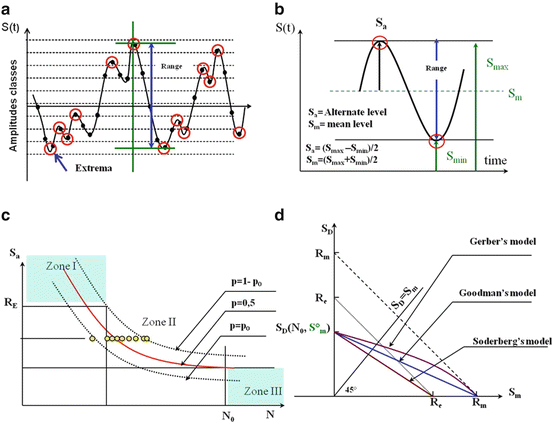

  

  The four steps of predicting of the lifetime. (a) Random stress, (b) after counting, (c) probabilized Wöhler’s curve, (d) fatigue criteria

• An endurance law (often based on the Wöhler) (Fig. 31c). Tests conducted for an average stress S ⁰_m zero and a stress S _a give results with different numbers of cycles to failure. The distribution is represented by a sequence of points. The different values of stresses are considered. Thereafter, the three curves can be derived with, respectively, p _r  = 50 %, p ₀, and 1 − p ₀ of failure probability. Typically, p ₀ is between 1 and 10 %.

• A fatigue requirement that sets the limit resistance (Fig. 31d). When the mean stress is not zero, the fatigue limit S _D depends on the value of the mean stress S _m, different models can then be used according to the stress S _m between 0 and R _E or R _m.

• A law of accumulation of damage to account for all the stresses applied to the system or component. Generally, it is the law that is used Miner.

5.1.2 Fatigue and Damage in the Lifetime Validation of a Mechanical Component

The results of the analysis of the stresses measured under actual conditions of use should be exploitable by the steps of the method of calculating the lifetime. Thus, we must find (Sect. 1) counting method for identifying a “statistical load event” in a random loading history. For example, the event may consist of amplitudes of grouped into classes, the extrema, stretches or “cycles” of the stress studied. Often, they are extended or stress cycles which are operated to perform the calculation of a lifetime.

To strengthen the capacity of prediction, calculation of lifetime must have a probabilistic approach to announce reliability. Rather than events or extended cycle type, the load events are grouped into classes where these are the extrema which are better suited to probabilistic modeling (Sect. 2).

5.1.2.1 Endurance Law or Wöhler Curve

A Wöhler curve (Fig. 31c) represents a probability p to rupture, the magnitude of the cyclic stress ((S _a) considered average for a given stress S _m) based on the lifetime N. Also known as curve S–N (Stress–Number of cycles).

The test conditions must be fully specified in both the test environment and the types of stress applied. Rupture occurs for a number of cycles increases when the stress decreases.

There are several models of these curves according to an endurance limit implicitly or explicitly appears. Indeed, when a material is subjected to low-amplitude cyclic stress, fatigue damage can occur for large numbers of cycles. Points of the curve of Wöhler are obtained with the results of fatigue tests on specimens subjected to cyclic loading of constant amplitude.

The curve is determined from which each batch of sample is subjected to a periodic stress maximum amplitude S _a and constant frequency, the failure occurring after a number of cycles N. Each sample corresponds to a point in the plane (S _a, N).

The results of the fatigue tests are randomly distributed, such that one can define curves corresponding to given failure probabilities according to the amplitude and the number of stress cycles.

This finding requires the construction of a model to the median (p _r  = 0.5, 50 % of failures) observed lifetimes, curves at p ₀ and at (1 − p ₀) are then deducted p ₀ is often taken equal to 0.01 (1 % of failures). These curves are called the Wöhler curves probabilized.

Wöhler curves are generally broken down into three distinct areas (Fig. 31c):

• Area I: Area of oligocyclic plastic fatigue, which corresponds to the higher stresses above the elastic limit R _E of the material. Breaking occurs after a small number of cycles typically varying from one cycle to about 10⁵ cycles.

• Area II: Area of fatigue or limited endurance, where the break is reached after a limited number of cycles (between 10⁵ and 10⁷ cycles).

• Area III: Area of endurance unlimited or safety area under low stress, for which the break does not occur after a given number of cycles (10⁷ and even 10¹⁰), higher the lifetime considered for the part.

In many cases, an asymptotic horizontal branch to the curve of Wöhler can be traced: the asymptote is called endurance limit or fatigue limit and denoted S _D. The latter is defined at zero mean stress (S ⁰_m  = 0) and corresponds to a lifetime N ₀ (N ₀ = 10⁷ cycles often).

In other cases, a conventional endurance limit may be set for example to 10⁷ cycles.

Generally, you must use a model that approximates the curves to perform further calculations. Various expressions have been proposed to account for the shape of the curve of Wöhler (Lieurade 1980b). The most practical was proposed by Basquin and she wrote as follows:

$$ N{S}^b={C}_1 $$

(69)

and

$$ \log N+ b \log S= C\left( C= \log \left({C}_1\right)\right) $$

(70)

With N = number of cycles, S = amplitude of the stress, b = slope of the line depends on the material, C = constant dependent right material and the average of the alternating stress fatigue test performed.

In the following text, the coefficient C will be used.

Fatigue tests are usually long term and it is rare to have the results of experiments conducted with a nonzero mean stress.

The increase in mean stress causes a reduction of the lifetime: a network of Wöhler curves can be thought (Fig. 32). Thus, the endurance limit for a chosen number of cycles (e.g., to N ₀ = 10⁷ cycles) decreases. Then, for each nonzero average stress, an endurance limit should be determined. Lacking often experimental results, the calculation is based on a relationship called “fatigue requirement.”

Fig. 32

Influence of mean stress on the network Wöhler curves

5.1.2.2 Fatigue Requirements

A fatigue test is a threshold defined by a mathematical expression for a fixed lifetime (N ₀) and a given material. The threshold separates the state where the part is operating in the state where it is damaged by fatigue.

In general, a fatigue test was developed for cyclic loading with constant amplitude.

It is a relationship between the evolution of the Wöhler curve and the average stress considered. Figure 31d shows the main criteria of fatigue. These graphs are built with a lifetime N ₀ (often given as 10⁷ cycles) and a given probability of failure (p _r  = 0.5, 0.1, and 0.01). These different models are (Rabbe et al. 2000b):

$$ \mathrm{Goodman}\ \mathrm{model}\kern1em {S}_{\mathrm{D}}={S}_{\mathrm{D}}^{*}.\left(1-\frac{S_{\mathrm{m}}}{R_{\mathrm{m}}}\right) $$

(71)

$$ \mathrm{Soderberg}\ \mathrm{model}\kern1em {S}_{\mathrm{D}}={S}_{\mathrm{D}}^{*}.\left(1-\frac{S_{\mathrm{m}}}{R_{\mathrm{E}}}\right) $$

(72)

$$ \mathrm{Gerbermodel}\kern1em {S}_{\mathrm{D}}={S}_{\mathrm{D}}^{*}.\left(1-{\left(\frac{S_{\mathrm{m}}}{R_{\mathrm{m}}}\right)}^2\right) $$

(73)

With S ^*_D  = S _D(S ⁰_m  = 0; N ₀) endurance limit defined for zero mean stress and number of cycles N ₀ selected.

Then, for a given cycle (amplitude, a range) having a nonzero mean, these relationships allow to obtain approximate the endurance limit for the average stress.

5.1.2.3 Calculation of Fatigue Damage, of Damage Accumulation, and of Lifetime

The concept of damage represents the state of degradation of the material in question. This condition results in a quantitative representation of the endurance of materials subjected to various loading histories.

A law of accumulative damage is a rule to accumulate damage variable D (also called “damage D”), itself defined by a law of damage.

As for the lifetime is defined by a number of cycles N which leads to breakage.

Thus, the application of n cycles (n < N) causes a partial deterioration of the treated piece to the calculation. The assessment of damage at a given time is crucial to assess the remaining capacity of lifetime.

Fatemi and Yang (Fatemi and Yang 1998) identified in the literature more than 50 laws of accumulated damage. The most commonly used today is the law of linear cumulative damage to Palmgren–Miner remains the best compromise between ease of implementation and the quality of predictions for large lifetimes (Banvillet 2001). Miner’s rule is as follows:

$$ {d}_i=\frac{n_i}{N_i} $$

(74)

With n _i  = the number of repetitions of a given cycle (with amplitude or extended), N _i  = the number of repetitions of the same cycle necessary to declare the failed component (n _i  < N _i ).

For different cycles of random stress studied, the global damage is obtained by linear addition of the elementary damage:

$$ D={\displaystyle \sum_i{d}_i}={\displaystyle \sum_i\frac{n_i}{N_i}} $$

(75)

Fracture occurs when D is 1. The lifetime is equal to 1/D.

5.1.2.4 Introductory Examples

The different steps of the calculation will be presented with a A42FP case (Leluan 1992b) steel. Figure 33 shows the model Basquin concerning fatigue tests on this steel with alternating stresses whose average is zero. Figure 34 shows the various criteria of fatigue such as steel. An endurance limit calculated from the right Soderberg is lower than those obtained with the right Goodman and the parabola of Gerber.

Fig. 33

Basquin Model of the Wöhler curve for Steel A42FP (from Leluan (1992b))

Fig. 34

Criteria of fatigue for Steel A42FP

This difference between endurance limits calculated using criteria of fatigue leads to some significant differences on the calculated life.

Example 1

The first question in this introductory example is how to calculate the damage suffered by the steel A42FP subjected to a stress of 10⁷⁵ cycles, the alternating stress (S _a) is 180 MPa, and mean stress (S _m) of 100 MPa, calculating with a failure probability of 0.5. The second question is to determine the number of repetitions of this stress must be applied for failure:

• Step 1: Calculation of the new endurance limit, according to each criteria of fatigue:

  Criteria of fatigue	S D (S m = 100 MPa; N = 107)
  Gerber parabola	203 MPa
  Goodman right	164 MPa
  Soderberg right	151 MPa

• Step 2: Calculation of the new constant C in the model Basquin:

  Criteria of fatigue	C(S m = 100 MPa; S D) = N × (S D)b = 107(S D)b
  Gerber parabola	2.45 × 1043
  Goodman right	8.45 × 1041
  Soderberg right	2.39 × 1041

• Step 3: Calculation of the number of cycles to failure for the stress studied according to the criteria of fatigue. In this case, the calculation is performed at 50 % of probability of failure:

  Criteria of fatigue	N = C × (S a)b
  Gerber parabola	9.15 × 1078
  Goodman right	3.16 × 1077
  Soderberg right	8.93 × 1076

• Step 4: Calculation of damage due to studied stress and the lifetime expectancy. Determination of the number of repetitions to reach failure

  Criteria of fatigue	D = n/N = 1075/N	Lifetimea = 1/D
  Gerber parabola	1.093 × 10−4	9,150 times
  Goodman right	3.16 × 10−3	316
  Soderberg right	1.12 × 10−2	89

  ^aThis result means that the stress will be able to repeat before reaching failure = number of repetitions.

In the case of multilevel constraints, these four steps of calculation (Example 1) are applied for each level and the total damage is obtained according to the rules of linear cumulative damage Miner.

Example 2

It involves the stress of an axle front right of the vehicle. Figure 35 shows the distribution of damage per area of the Markov matrix for stress shown in Fig. 10 (Kouta and Play 2007a). The total damage is 6.05 E-06 and the number of repetitions of this stress before reaching failure is 165,273 times. The separation of Fig. 35 in eight zones ((a)–(h)) allows to visualize the contribution of the elementary stresses.

Fig. 35

Distribution of damage per area of the Markov matrix (stress shown in Fig. 10, part 1)

The nature of the stresses together in each area specified in Fig. 9. Fifteen percent of damage in the area (a) of Fig. 35 can be explained mainly by effective stress that are at the end of the Markov matrix (top right of Fig. 10).

Among a workforce of N = 15, a workforce of 5 (2 + 2 + 1) corresponds to the five largest observed this stress extended. These result from extensive shocks when moving the vehicle in five concrete bumps. A total of 17.7 % of the damage area of the figure reflects the severity of the extended amplitude whose average is positive. They reflect the effect of compression after passing on concrete bumps.

5.1.3 Contributions and Impact of a Statistical Modeling for Random Loading in the Calculation of Lifetime

5.1.3.1 Principle of Damage Calculating

Data around which theoretical models of probability density are of three kinds (part 1):

• The amplitudes grouped into classes.

• Extreme amplitudes.

• Envelope of the stress.

Thus, three models of calculation will be presented in the following paragraphs. The evolution of damage is always calculated from the model Miner. We write an element of damage by fatigue dD is due to a stress element dn. Under the law of Miner

$$ dD=\frac{dn}{N(S)} $$

(76)

with dn number of amplitudes solicitation studied at the level between S and S + ds.

• For a given duration T,

  $$ dn={N}_T\times {f}_S(s)\; ds, $$

  with N _T the total number of stresses and f _S (s) probability density of the time stress whose level is equal to S.

• To stress measured with a time step Δt = 1/f _e (f _e sampling frequency), the total number of stresses is equal to N _T  = f _e  × T. Thus, the global damage is the sum of the partial damage for all values f S:

  $$ D={N}_T\times {\displaystyle \underset{\Delta}{\int}\frac{f_S(s)}{N(S)}\times ds} $$

  (77)

  with Δ = domain of definition of S.

• Where the Wöhler is regarded as the model Basquin:

  In this case, (NS ^b = C, C is a constant depending on the level of stress), Eq. (76) becomes:

  $$ D=\frac{N_T}{C}\times {\displaystyle \underset{\Delta}{\int }{s}^b}\times {f}_S(s)\times ds $$

  (78)

  If we set

  $$ u=\frac{s}{\sqrt{V(S)}} $$

  with V(S) variance S. Relation Eq. (78) is written:

  $$ D={\left[ V(S)\right]}^{b/2}\frac{N_T}{C}\times {\displaystyle \underset{\Delta}{\int }{u}^b}\times {f}_U(u)\times du $$

  (79)

  Thus, the damage is D calculated for each amplitude family around which a probabilistic modeling is proposed (Sect. 1). Firstly, the calculation can be done according to the system of Pearson (Beta 1 law, Beta 2 law and Log-Normal law, Gamma Law and Weibull law, Normal (or Gaussian) law. Calculation can also be done using either the law of Gram-Charlier–Edgeworth or the law of the envelope (or Rice).

5.1.3.2 Damage Calculating on the Basis of Laws Obtained by Pearson System

Table 5 gives the result of the relationship Eq. (79), obtained by the Pearson system for each probability law or each equivalent law. The laws of probability so that their parameters are given in Appendix 1.

Table 5 Calculation of damage according to the Pearson system (see Fig. 36)

Figure 36 shows the influence of parameters that define the laws of probability on the global damage. It is clear that the damage D decreases with increasing exponent b because when b increases (for a given C), the lifetime increases with the model Basquin.

Fig. 36

Evolution of damage depending on the settings of each probability distribution. (a) Damage with Beta 1, (b) damage with Beta 2, (c) damage with gamma, (d) damage with Weibull, (e) damage with Log Normal, (f) damage with Gauss

5.1.3.3 Damage Calculating on the Basis of the Gram-Charlier–Edgeworth Law

In this case, the calculation from Eq. (79) is performed with the probability density function expressed with Eq. (11). Equation (79) leads to the following Eq. (86):

$$ D={\left[ V(S)\right]}^{b/2}\frac{N_T}{C\sqrt{2\pi}}\left\{\begin{array}{l}\gamma \left(\frac{\left(1+ b\right)}{2}\right)\left(1+{\left(-1\right)}^b\right).\left\{\begin{array}{l}{2}^{\left(\frac{b-1}{2}\right)}+{2}^{\left(\frac{b+1}{2}\right)}\\ {}\times \left[\left(\frac{k_3^2 b}{18}\right)+\left(\frac{k_3^2{b}^2}{14}\right)+\left(\frac{k_4{b}^2}{48}\right)-\left(\frac{k_4 b+{k}_3^2{b}^2}{24}\right)\right]\end{array}\right\}\\ {}+\gamma \left(\frac{b}{2}+1\right){2}^{\frac{b}{2}}{k}_3\left(\frac{b-1}{6}\right)\left(1-{\left(-1\right)}^b\right)\end{array}\right\}$$

(86)

Figure 37 shows the evolution of the damage function of b, the skewness β ₁, and β ₂ kurtosis of the stress distribution. All curves decrease with the increase of the parameter b. For a given β ₁ parameter when kurtosis β ₂ increases, that is to say, the dispersion of the stress distribution and damage increases, when the skewness ratio increases, the damage also.

Fig. 37

Evolution of damage according to the law of Gram-Charlier–Edgeworth

5.1.3.4 Damage Calculating on the Basis of the Rice Law on the Envelope

The presented model of the envelope in Sect. 2.4 and Appendix 5 relates extrem amplitudes, so the total number of stresses is equal to the number N _T extrem amplitudes N _e. In this case, the damage is determined by the relationship

$$ D\approx \frac{{\left[ V(S)\right]}^{\frac{b+1}{2}}{N}_{\mathrm{e}}}{C}\kern0.5em \left\{\begin{array}{l}\frac{2^{\frac{b}{2}-1}{\left(1- I \mathit{^2}\right)}^{\frac{b}{2}+1}\gamma \left(\frac{b+1}{2}\right)}{\sqrt{\pi}}+{2}^{\frac{b}{2}-1} I\gamma \left(\frac{b}{2}+1\right)\\ {}+\frac{2^{\frac{b+1}{2}}{I}^3}{\left(1- I \mathit{^2}\right)\sqrt{\left( b+2\right)\pi}}\varPhi \left(\frac{2 I \mathit{^2}}{1- I \mathit{^2}};1;\left[ b+2\right]\right)\end{array}\right\} $$

(87)

With Φ (x, 1, [b + 2]) is the cumulative probability function of Fischer–Snedecor of x in the degrees of freedom with one and the integer part of (b + 2).

Note Φ(0, 1, [b + 2]) = 1 and Φ(∞, 1, [b + 2]) = 0. The results for the particular case of irregularity factor I are presented in Table 6:

Table 6 Calculation of damage to individual cases of irregularity factor I

The damage curves (Fig. 38) decrease as the parameter b is increased (slopes substantially equal to the slopes Fig. 37). When the irregularity factor changes from 0 (broadband) to a value of 1 (narrowband), damage increases. This effect is due to the increased number of cycles with a narrowband signal.

Fig. 38

Evolution of damage according to the law of the envelope of Rice

5.1.3.5 Applications (Brozzetti and Chabrolin 1986b)

Fatigue strength of a node type T “jacket” of an “offshore” structure must be checked. Available records concerning the height of the waves beat structure; values are based on the frequency of occurrence (Table 7). These records are related to a reference time of 1 year.

Table 7 Frequency of occurrence of solicitation for a T structure

At each of these wave heights, the calculation of the structure leads to a stress on the design of the T node (Δσ, in MPa, Table 7). This constraint sizing takes into account a coefficient of stress concentration T node considered.

Fatigue curve at 50 % of the considered node failures is given by the expression (Basquin deviation) as follows:

$$ N\Delta {\sigma}^{10}={10}^{10}\kern1em \mathrm{or}\kern1em \log (N)=-3 \log \left(\Delta \sigma \right)+10 $$

(90)

Fatigue curve 1 % failure is as follows: NΔσ ^2.9 = 10^9.8. These curves are presented in Fig. 39.

Fig. 39

Endurance curve (for T type node jacket) of an offshore structure

Calculation of cumulative damage to the node as well as its lifetime can be made using the methods presented in the previous sections.

5.1.3.5.1 Calculation of Damage and Lifetime According to the Classical Method

Table 8 presents the calculation of cumulative damage by applying Miner’s rule (“Calculation of fatigue damage, of damage accumulation and of lifetime” and “Introductory examples” in Appendix E). The accumulated damage of the fatigue curve with 50 % of failures provides a value D _(0,5) = Σ(n _i /N _i ) = 0.0147 and the lifetime of the node = 1/D = 68 years. The calculation with the fatigue curve gives 1 % damage D _(0,01) = 0.0193 so a minimum lifetime of 52 years.

Table 8 Damage and lifetime for a T structure

This approach to calculation is based on the observed numbers (n _i ) and the lifetime limit estimated (N _i ) for each level of the stress concerned. The statistical nature of the distribution of staff (or the probability amplitudes of the stress studied) is not taken into account. Moreover, this calculation of the global lifetime of endurance depends on the model given in Eq. (90).

5.1.3.5.2 Calculation of Damage and Lifetime by Statistical Modeling

The process of calculation, in this paragraph, incorporates the statistical nature of the distribution of staff (or the probability amplitudes of the stress studied) and uses the same model of endurance expressed by Eq. (90). In this case, the damage is assessed from the following four elements:

• Law of distribution of wave heights in the long term

  In this example, distribution of wave heights corresponds to a Weibull law:

  $$ H={H}_0+{p}_{\mathrm{cte}} \log (n). $$

  (91)

  With H ₀ is the maximum wave height recorded in the reference period (within 1 year); n is the number of wave heights greater than H ₀, p _cte is a constant.

• Damage law (or curve of fatigue or S–N curve)

  $$ \mathrm{Let}:\kern0.5em N\Delta {\sigma}^b= C,\kern0.5em \mathrm{let}: N= C\Delta {\sigma}^{- b}\left(\mathrm{same}\kern0.5em \mathrm{Eq}.\kern0.5em (90)\right) $$

  (92)

  With b = slope of the S–N curve, N = number of cycles associated with the variation of the stress sizing Δσ, Δσ extent of stress variation in the node in T of the structure.

• Relationship between wave height H to the stress variation Δσ

  The stress variation Δσ is laid as:

  $$ \Delta \sigma =\alpha.{H}^{\beta} $$

  (93)

  with α and β two coefficients that are obtainable by smoothing spots (Δσ, H).

  If the value of Δσ given by the expression Eq. (93) in Eq. (92) is postponed, we obtain:

  $$ N= C\alpha.{\left({H}^{\beta}\right)}^{- b} $$

  (94)

  Transformation of expression Eq. (91) gives:

  $$ n={n}_0. \exp \left(2.3026 H/{p}_{\mathrm{cte}}\right) $$

  (95)

  With ${n}_0={10}^{-{H}_0/{p}_{\mathrm{cte}}}$.

• Rule of damage cumulation

  $$ \Delta D= dn/ N $$

  (96)

  Thus,

  $$ dn=\left(2.3026/{p}_{\mathrm{cte}}\right){n}_0 \exp \left(2.3026 H/{p}_{\mathrm{cte}}\right)\; dH $$

  (97)

  We obtain:

  $$ \Delta D= dn/ N={\alpha}^b\left(2.3026/ C.{p}_{\mathrm{cte}}\right){n}_0 \exp \left(2.3026 H/{p}_{\mathrm{cte}}\right){H}^{b\beta}\; dH $$

  (98)

  Let:

  $$ D=\frac{2.3026{n}_0{\alpha}^b}{C.{p}_{\mathrm{cte}}}\kern0.2em {\displaystyle \underset{0}{\overset{\infty }{\int }} \exp \left(\frac{2.3026\kern0.2em H}{p_{\mathrm{cte}}}\right){H}^{b\beta}\; dH} $$

  (99)

  $\mathrm{We}\;\mathrm{recall}\kern0.5em \mathrm{that}:{\displaystyle {\int}_0^{\infty }{t}^u \exp \left(- v{t}^w\right) dt}=\frac{\gamma \left[\left( u+1\right)/ w\right]}{w{ v}^{\left( u+1\right)/ w}}$; γ(t) is the gamma function (see Eq. (28)) with u = βbv = 2.3026/p _cte and w = 1, we obtain

  $$ D=\frac{2.3026{n}_0{\alpha}^{- b}}{C.{p}_{\mathrm{cte}}}\kern0.1em \frac{\gamma \left(\beta b+1\right)}{{\left(\frac{2.3026}{p_{\mathrm{cte}}}\right)}^{\left(\beta b+1\right)}} $$

  (100)

Example 3

From the data in Table 7, we obtain by smoothing:

$$ H=6.1+0.913 \log (n)\kern0.5em \left( H\;\mathrm{in}\;\mathrm{meters}\right)\kern1em \Delta \sigma =3.9{H}^{1.2}. $$

Let: α = 3.9; β = 1.2; b = 3; p _cte = 0/913; C = 10¹⁰; H ₀ = 6.1; n ₀ = 10^6.1/0.913.

Hence: γ(bβ + 1) = γ(4,6) = 13.38; α ^b = 59.32; 2.3026n ₀ = 11,053,226; p _cte. C = 0.913 × 10¹⁰.

Thus, damage: D = 0.0137.

So the lifetime is 1/D = 73 years.

With the model of endurance to 1 % failure (NΔσ ^2.9 = 10^9.8), the lifetime is equal to 49 years.

In summary for this application (see Table 9), the transition from a traditional approach to statistical modeling provides a better prediction of behavior (7 % saving). It is also noted that the increase of reliability of from 0.5 to 0.99 decreases calculated lifetime to about 28 %.

Table 9 Summary of results for structure T application

5.1.4 Calculation of Damage and Lifetime on the Basis of Power Spectral Density (Lalanne 1999b)

A system or a mechanical component has a response to applied stresses (PSD). This response can be either measured on a prototype under tested qualification, either calculated from a global mechanical model.

The expression Eq. (79) shows that the damage depends on the variance of the amplitudes of the stress. The relation Eq. (46) gives the expression for the variance of a random stress according to its PSD. It must be previously represented by several levels (G _i ). In this case, the relation Eq. (79) is then expressed as follows:

$$ D=\frac{N_T}{C}{\left[ V(S)\right]}^{b/2}{\displaystyle \underset{\Delta}{\int }{u}^b{f}_U(u)\; du}=\frac{N_T}{C}.{\left[\frac{\frac{\pi}{4\xi}{\displaystyle \sum_{i=1}^n{G}_i\left[{I}_0\left({h}_{i+1}\right)-{I}_0\left({h}_i\right)\right]}}{{\left(2.\pi \right)}^4{f}_0^3}\right]}^{b/2}{\displaystyle \underset{\Delta}{\int }{u}^b{f}_U(u)\; du}$$

(101)

• This expression is called “Fatigue Damage Spectrum” (Lalanne 1999b). The terms ${\displaystyle \underset{\Delta}{\int }{u}^b{f}_U(u)\; du}$ and $\frac{N_T}{C}$ are two multiplicative constants of the term expressed in the brackets of the expression Eq. (101). This term represents the evolution of the variance of the stress according to the frequencies.

• Figure 40 shows the next term $\frac{N_T}{C}{\left[ V(S)\right]}^{b/2}$ of the Fatigue Damage Spectrum on the stress shown in Fig. 10. This graph is obtained for C = 10⁷ and b = 12, the value of b is given by (Lambert 1980) as an average value of the slope of the line for Basquin steels. The failure probability is 1 %. In Fig. 40, there is not a particular representative value to summarize the shape of the curve. However, an average value may be deducted, equal to 7.77 × 10⁻⁹ (the minimum is 5.89 × 10⁻⁴¹ and the maximum is 1.83 × 10⁻⁰⁶).

  Fig. 40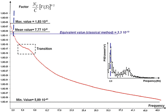

  

  Fatigue damage spectrum depending on the frequency

• The value of the term ${\displaystyle \underset{\Delta}{\int }{u}^b{f}_U(u)\; du}$ depends on the model probability density which is adopted for the stress studied. In the case of a Gaussian distribution, this sum is $\frac{2^{\frac{b}{2}}}{\sqrt{2\pi}}\gamma \left(\frac{b+1}{2}\right)$ (see relation Eq. (85)). The value here is equal to 18,425 (for b = 12). Thus, the average damage D _av is 1.43 × 10⁻⁴ (with a minimum damage equal to 1.09 × 10⁻³⁶ D _min and D _max maximum damage equal to 3.37 × 10⁻²). The lifetime (or the number of repetitions to failure 1/D _av) is equal to 6,993.

• This calculation of the lifetime by the PSD as takes into account all the contributions of the stress on the frequency domain of stresses. The shape of the Fatigue Damage Spectrum is thus brought into relationship with the shape of the PSD (Power Spectral Density). The PSD of the stress studied (Fig. 13b) is outlined in Fig. 40. Thus, the almost flat spectrum observed in the fatigue damage in the area of transition nature (framed part in Fig. 40) is due to the transition between the two major contributions observed on the PSD. These two are the two main modes, the stress observed studied.

• Note that the damage calculation by conventional method (described in “Calculation of fatigue damage, of damage accumulation and of lifetime” and “Introductory examples” in Appendix 5) gives damage D _conventional equal to 6.05 × 10⁻⁶. This level of damage is equivalent value $\frac{N_T}{C}{\left[ V(S)\right]}^{b/2}=3.3\times {10}^{-10}$, value that is located in the terminals and mini max damage (Fig. 40).

However, conventional method gives a value of damage to a single class of frequency (around 2 Hz) corresponding to the largest amplitudes of the PSD. Lifetime (or the number of repetitions before failure 1/D _conventional) is then equal to 165,273 repetitions. The difference between the result of the lifetime by PSD and that obtained by the conventional method is now 95 %, results become very different.

Result obtained with Fatigue Damage Spectrum allows differentiation the role of each frequency band to obtain the damage. Damage results consequences of any stresses represented by the spectral density PSD. Damage obtained by this method takes into account all frequency levels that appear with their stress levels and their respective numbers.

5.1.5 Plan of Validation Tests

The different models presented to assess the damage and the lifetime in real use conditions based on different types of analysis of stresses measured on a system or a mechanical component. These models also allow defining test environments that must cause similar effects to those observed in the actual conditions of use.

• The experimental means perfect more and more to reproduce in laboratory the stresses recorded in real conditions of use. These types of tests are designed to validate models of mechanical calculation and are not intended to validate the lifetime estimated by the models presented earlier. Such validation would require too much time. Indeed, the need to reduce more and more the validation period of a product required to do as much as possible, test duration shorter and shorter and more severe than the stress level observed in the actual conditions of use. Naturally, these severe tests shall show equivalent to those observed in real use conditions consequences.

  Damage is an equivalence indicator.

• Figure 41 illustrates the principle of equivalent damage. In the case of alternating stresses and with a material whose curve of resistance to fatigue (Wöhler curve) is known, the limit lifetime is expressed in terms of alternating stress of solicitation. If we assume that the actual conditions of use are summarized in n _real repetitions of a sinusoidal stress (S _a = S _real) which is N _real the limit lifetime in these conditions of use (n _real < N _real). In this case (according to Miner), damage under real conditions of use is: ${d}_{\mathrm{real}}={\scriptscriptstyle \frac{n_{\mathrm{real}}}{N_{\mathrm{real}}}}$.

  Fig. 41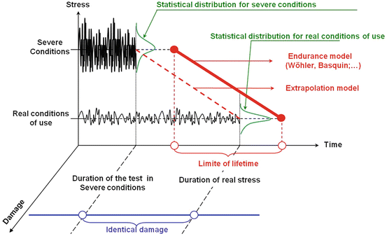

  

  Schema of the principle of equivalent damage

• Conducting a test in more severe conditions and leads to the same level of damage d _real is to define the number of times (n _severe) to be repeated a sinusoidal stress (S ^′_a  = S _severe) so that the damage d _severe is equal to d _real.

• For a mechanical component, the level (S ^′_a  = S _severe) is determined depending on the material which constitutes the studied and knowledge about limits behavior component. The equivalence between damage (d _severe = d _real) leads to the calculation of n _severe. As follows:

  $$ {n}_{\mathrm{severe}}={\scriptscriptstyle \dfrac{N_{\mathrm{severe}}}{N_{\mathrm{real}}}}{n}_{\mathrm{real}} $$

  (102)

  According to the model Basquin N = CS ^−b, then

  $$ {n}_{\mathrm{severe}}={\left(\frac{S_{\mathrm{severe}}}{S_{\mathrm{real}}}\right)}^{- b}{n}_{\mathrm{real}} $$

  (103)

  Figure 42 illustrates the process of calculating the number of cycles required to produce, under severe conditions, damage equivalent to that observed under actual use conditions.

  Fig. 42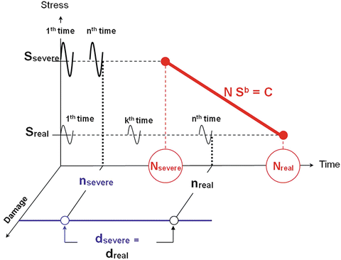

  

  Schema of the equivalent damage principle in the case of sinusoidal stresses

• A detailed analysis of behavior in endurance (long period) should help define tests (short term) to perform in laboratory or on simulation bench. In this case, it is advisable to retain only the critical stresses. Two selection criteria are possible: take only the stresses that have contributed from a given percentage of the global damage or take the stresses whose amplitude alternating (S _a, Fig. 31b) is greater than the limit endurance.

  For the examples presented in the following, this is the second criterion that is used.

  • Figure 43 shows the transition matrix corresponding to the stress of Fig. 40 by specifying the boxes (with gray background) in which the associated alternating stress is below the endurance limit. If these stresses are not considered, the cumulative damage remaining 72 % of the global damage.

    Fig. 43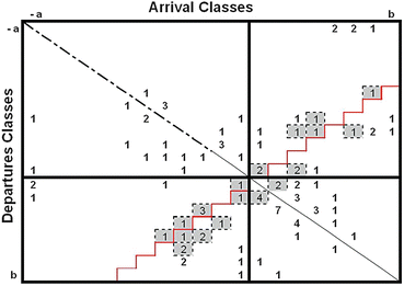

    

    Transition matrix of the stress with distinction parts of the alternating stresses which amplitude is less than the endurance limits (see Fig. 10)

  • The remaining part of the transition matrix can be used for testing in the laboratory. Of course, it is only the nonempty boxes of the matrix are taken into account.

  • In the case of this stress, the information obtained by the extended-slope matrix (Fig. 21a) and the extreme-curves matrix (Fig. 21b) contributes to the definition of the dynamic sinusoidal stresses considered for each nonempty cell of the matrix of transition.

  • In the top right quarter of the matrix linking extreme amplitudes and curvatures (Fig. 21b), there is five number which summarizes the five extreme amplitudes (negative) observed following the passage of the five concrete bumps. Based on the transition matrix (Fig. 10), these five amplitudes are the starting points of which types of stress do not have exactly the same end point. But the information provided by the extreme-curvature matrix confirms that these five amplitudes the frequency signature is identical.

  • The frequency according to which occur these five amplitudes is calculated as:

    $$ \mathrm{frequence}=\frac{1}{2\pi}\sqrt{\left|\frac{y^{{\prime\prime} }}{y}\right|} $$

    (104)

    with y ^″ is the second derivative of the signal y of load plotted against time.

  • This relationship can also calculate all the frequencies of stresses that must be applied during laboratory tests. These are the quarters on up and right and down left of the extremes-curvatures matrix which are favored because they plot stresses whose sign of the amplitude of departure is different from the amplitude of arrival, reflecting extent of high amplitude. The quarters up left and down right plot intermediate fluctuations which are not important as long as they remain concentrated around the center of the matrix.

• The transition matrix of Fig. 44a shows a stress history near a fillet weld on a transport vehicle chassis (Kouta et al. 2002) in an actual path of usage of 464 km. Figure 44b shows this same matrix in the form of Iso-curves (or level curves). This second representation gives iso-level curves of log of numbers, for an easier viewing. In red (center of the butterfly), there are more effective but they are the least damaging. By against in blue, the lowest numbers are shown but the most damaging. For this case of loading, figure is symmetrical with respect to the first diagonal, and is offset slightly downwardly. Note also the existence of two small separate areas from the main figure.

  Fig. 44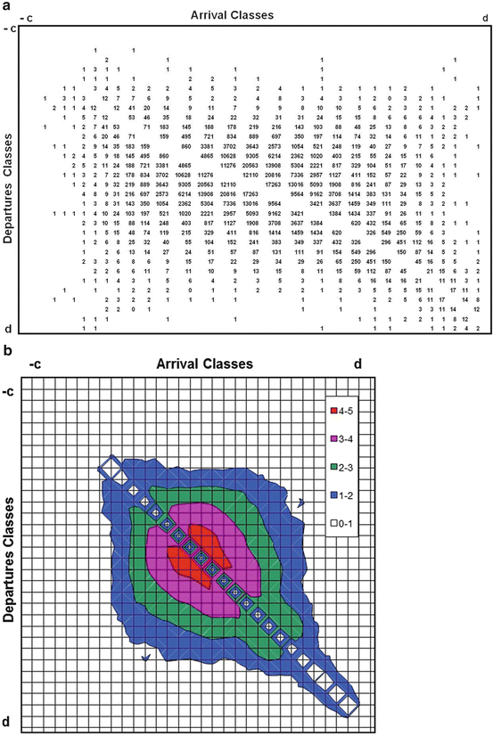

  

  Two representations (a stress history and b iso-curves) of a transition matrix for a fillet weld of the bogie chassis (according to (Kouta et al. 2002))

  • A first failure on the ground was observed on this path of 464 km after 1E + 06 km (2,155 rehearsals). Endurance characteristics of the material (Wöhler curve) were determined through laboratory tests on this type of component. The calculation of lifetime through the approach presented earlier (“Calculation of fatigue damage, of damage accumulation and of lifetime” and “Introductory examples” in Appendix 5) leads to a calculated lifetime of 1.2E + 06 km, which was satisfactory.

• The conditions of an endurance test of short-term representative of the actual damage were defined from Eq. (103). Figure 45 shows the transition matrix corresponding to an endurance test which is obtained with a ratio of severity equal to 2 {(S _severe/S _real) = 2, amplitude −2c, +2d}. This matrix provides the same damage as observed by considering the matrix in Fig. 44 but with a test duration which corresponds to a distance of 5 km with a rehearsal. Thus, this new matrix can be used to achieve a short-term endurance test in laboratory whose consequences (analysis of cracks, probable failure, etc.) are representative of a real long-term use.

  Fig. 45

  

  Transition matrix corresponding to an endurance test obtained with a ratio of severity equal to 2 from the matrix in Fig. 43 (Matrix obtained under the rule of equivalent damage, see Eq. (102))

5.1.6 Conclusion

The approach presented in three parts was motivated by the challenges of quality requirements for mechanical systems and components. And more specifically, lifetime and reliability (probability of no break) are two main features. All of the tools can be naturally applied to all cases of random stresses in mechanical. Engineers of design and development in mechanical have to know in detail:

• Actual conditions of use from users’ behaviors.

• Actual conditions of use from users’ behaviors.

• Behaviors (or responses) of studied systems.

• Models of material degradation.

Thus achieve the provision of values lifetime is not an insurmountable task. However, numerical results should always be viewed and analyzed the same time as the assumptions that lead to their obtaining.

Different approaches for calculating lifetime were presented as well as intermediate hypotheses required to calculate:

• Approach with statistical modeling (“Contributions and Impact of a Statistical Modelling for Random Loading in the Calculation of Lifetime” section in Appendix 5) can now relay conventional approach (“Calculation of Fatigue Damage, of Damage Accumulation and of Lifetime” and “Introductory Examples” sections in Appendix 5) traditionally used in design departments. This approach with statistical modeling provides a global indicator of damage, lifetime, and reliability which remains easy to obtain while having improved the quality of behavior prediction.

• Approach Fatigue Damage Spectrum with the use of the PSD is however in conjunction with the actual conditions of use of mechanical systems and components. Fatigue Damage Spectrum whose the method of obtaining has been developed in “Calculation of Damage and Lifetime on the Basis of Power Spectral Density (Lalanne 1999b)” in Appendix 5, allows to connect lifetime (or damage) of a mechanical component with dynamic characteristics of stresses sustained by the material. The use of PSD in this calculation allows taking into account the dynamic behavior of the system which belongs to the mechanical component studied. In addition, this approach allows taking into account the nature of the statistical distribution of the solicitation.

• Validation of predictive calculations in systems and mechanical components design also calls for the establishment of specific test procedures. Naturally, market pressure requires test times which are compatible with the terms of product development. In general, these periods have nothing to do with expected lifetime in service. The obtained results allow constructing simple environments of bench testing of similar severity to that observed in tests of endurance.