Pebble minimization: the last theorems

Abstract

Pebble transducers are nested two-way transducers which can drop marks (named “pebbles”) on their input word. Such machines can compute functions whose output size is polynomial in the size of their input. They can be seen as simple recursive programs whose recursion height is bounded. A natural problem is, given a pebble transducer, to compute an equivalent pebble transducer with minimal recursion height. This problem has been open since the introduction of the model.

In this paper, we study two restrictions of pebble transducers, that cannot see the marks (“blind pebble transducers” introduced by Nguyên et al.), or that can only see the last mark dropped (“last pebble transducers” introduced by Engelfriet et al.). For both models, we provide an effective algorithm for minimizing the recursion height. The key property used in both cases is that a function whose output size is linear (resp. quadratic, cubic, etc.) can always be computed by a machine whose recursion height is 1 (resp. 2, 3, etc.). We finally show that this key property fails as soon as we consider machines that can see more than one mark.

1 Introduction

Transducers are finite-state machines obtained by adding outputs to finite automata. They are very useful in a lot of areas like coding, computer arithmetic, language processing or program analysis, and more generally in data stream processing. In this paper, we consider deterministic transducers which compute functions from finite words to finite words. In particular, a is a two-way automaton with outputs. This model describes the class of , which is often considered as one of the functional counterparts of regular languages. It has been intensively studied for its properties such as closure under composition [5], equivalence with logical transductions [12] or regular expressions [7], decidable equivalence problem [14], etc.

Pebble transducers and polyregular functions. can only describe functions whose output size is at most linear in the input size. A possible solution to overcome this limitation is to consider nested . In particular, the model of has been studied for a long time [13]. For $k=1$, a is just a . For $k \geqslant 2$, a is a that, when on any position i of its input word, can call a . The latter takes as input the original input where position i is marked by a “pebble”. The main then outputs the concatenation of all the outputs produced along its calls. The intuitive behavior of a is depicted in fig. 1. It can be seen as a recursive program whose recursion stack has height 3. The class of functions computed by is known as . It has been intensively studied due to its properties such as closure under composition [11], equivalence with logical interpretations [4], etc.

Fig. 1.

Behavior of a .

Optimization of pebble transducers. Given a computing a function f, a very natural problem is to compute the least possible $1 \leqslant \ell \leqslant k$ such that f can be computed by an . Furthermore, we can be interested in effectively building an for f. Both questions are open, but they are meaningful since they ask whether we can optimize the recursion height (i.e. the running time) of a program.

It is easy to observe that if f is computed by a , then $|f(u)| = \mathcal {O}(|u|^k)$. It was first claimed in a LICS 2020 paper that the minimal recursion height $\ell$ of f (i.e. the least possible $\ell$ such that f can be computed by an ) was exactly the least possible $\ell$ such that $|f(u)| = \mathcal {O}(|u|^{\ell })$. However, Bojańczyk recently disproved this statement in [3, Theorem 6.3]: the function can be computed by a and is such that , but it cannot be computed by a . Other counterexamples were given in [16] using different proof techniques. Therefore, computing the minimal recursion height of f is believed to be hard, since this value not only depends on the output size of f, but also on the word combinatorics of this output.

Optimization of blind pebble transducers. A subclass of , named , was recently introduced in [17]. A is somehow a , with the difference that the positions are no longer marked when making recursive calls. The behavior of a is depicted in fig. 2. The class of functions computed by is strictly included in [10, 17]. The main result of [17] shows that for , the minimal recursion height for computing a function only depends on the growth of its output. More precisely, if f is computed by a , then the least possible $1 \leqslant \ell \leqslant k$ such that f can be computed by an is the least possible $\ell$ such that $|f(u)| = \mathcal {O}(|u|^{\ell })$.

Fig. 2.

Behavior of a .

Contributions. In this paper, we first give a new proof of the connection between minimal recursion height and growth of the output for . Furthermore, our proof provides an algorithm that, given a function computed by a , builds a which computes it, for the least possible $1 \leqslant \ell \leqslant k$. This effective result is not claimed in [17], and our proof techniques significantly differ from theirs. Indeed, we make a heavy use of , which have already been used as a powerful tool in the study of [2, 8, 10].

Secondly, the main contribution of this paper is to show that the (effective) connection between minimal recursion height and growth of the output also holds for the class of (introduced in [13]). Intuitively, a is a where a called submachine can only see the position of its call, but not the full stack of the former positions. The behavior of a is depicted in fig. 3. Observe that a is a restricted version of a . Formally, we show that if f is computed by a , then the least possible $\ell$ such that f can be computed by a is the least possible $\ell$ such that $|f(u)| = \mathcal {O}(|u|^{\ell })$. Furthermore, our proof gives an algorithm that effectively builds a computing f.

Fig. 3.

Behavior of a .

As a third theorem, we show that our result for is tight, in the sense that the connection between minimal recursion height and growth of the output does not hold for more powerful models. More precisely, we define the model of , which extends by allowing them to see the two last positions of the calls (and not only the last one). We show that for all $k \geqslant 1$, there exists a function f such that $|f(u)| = \mathcal {O}(|u|^2)$ and that is computed by a , but cannot be computed by a . The proof of this result relies on a counterexample presented by Bojańczyk in [2].

Outline. We introduce in section 2. In section 3 we describe and . We also state our main results that connect the minimal recursion height of a function to the growth of its output. Their proof goes over sections 4 to 6. In section 7, we finally show that these results cannot be extended to two visible marks.

2 Preliminaries on two-way transducers

Capital letters A, B denote alphabets, i.e. finite sets of letters. The empty word is denoted by $\varepsilon$. If $u \in A^*$, let $|u| \in \mathbb {N}$ be its length, and for $1 \leqslant i \leqslant |u|$ let u[i] be its i-th letter. If $i \leqslant j$, we let u[i : j] be $u[i]u[i{+}1] \cdots u[j]$ (empty if $j <i$). If $a \in A$, let $|u|_a$ be the number of letters a occurring in u. We assume that the reader is familiar with the basics of automata theory, in particular two-way automata and monoid morphisms. The type of total (resp. partial, i.e. possibly undefined on some inputs) functions is denoted $S \rightarrow T$ (resp. $S \rightharpoonup T$).

The machines described in this paper are always .

Definition 2.1

A $\mathscr {T}= (A,B,Q,q_0,F,\delta ,\lambda )$ consists of:

• an input alphabet A and an output alphabet B;

• a finite set of states Q with $q_0 \in Q$ initial and $F \subseteq Q$ final;

• a transition function ;

• an output function with same domain as $\delta$.

The semantics of a $\mathscr {T}$ is defined as follows. When given as input a word $u \in A^*$, $\mathscr {T}$ disposes of a read-only input tape containing . The marks and are used to detect the borders of the tape, by convention we denote them by positions 0 and $|u|{+}1$ of u. Formally, a configuration over is a tuple (q, i) where $q \in Q$ is the current state and $0 \leqslant i \leqslant |u|{+}1$ is the position of the reading head. The transition relation is defined as follows. Given a configuration (q, i), let $(q',\star ):= \delta (q,u[i])$. Then whenever either and $i' = i{-}1$ (move left), or and $i' = i{+}1$ (move right), with $0 \leqslant i' \leqslant |u|{+}1$. A run is a sequence of configurations . Accepting runs are those that begin in $(q_0, 0)$ and end in a configuration of the form $(q, |u|{+}1)$ with $q \in F$ (and never visit such a configuration before).

The partial function $f: A^* \rightharpoonup B^*$ computed by the $\mathscr {T}$ is defined as follows: for $u \in A^*$, if there exists an accepting run on , then it is unique, and f(u) is defined as . The class of functions computed by is called .

Example 2.2

Let $\widetilde{u}$ be the mirror image of $u \in A^*$. Let $\# \not \in A$ be a fresh symbol. The function can be computed by a , that reads each factor $u_j$ from right to left.

It is well-known that the domain of a is always a (see e.g. [18]). From now on, we assume without losing generalities that our only compute total functions (in other words, they have exactly one accepting run on each ). Furthermore, we assume that for all $q \in Q$ (we only lose generality for the image of $\varepsilon$).

In the rest of this section, $\mathscr {T}$ denotes a with input alphabet A, output alphabet B and output function $\lambda$. Now, we define the in a position $1 \leqslant i \leqslant |u|$ of input . Intuitively, it regroups the states of the accepting run which are visited in this position.

Definition 2.3

Let $u \in A^*$ and $1 \leqslant i \leqslant |u|$ . Let be the accepting run of $\mathscr {T}$ on . The of $\mathscr {T}$ in i, denoted , is defined as the sequence .

If $\mu : A^* \rightarrow \mathbb {M}$ is a monoid morphism, we say that any $m,m' \in \mathbb {M}$ and $a \in A$ define a that we denote by $m {\boldsymbol{\llbracket } a\boldsymbol{\rrbracket }} m'$. It is well-known that the in a position of the input only depends on the of this position, for a well-chosen monoid, as claimed in proposition 2.4 (see e.g. [7]).

Proposition 2.4

One can build a finite monoid $\mathbb {T}$ and a monoid morphism $\mu : A^* \rightarrow \mathbb {T}$, called the of $\mathscr {T}$, such that for all $u \in A^*$ and $1 \leqslant i \leqslant |u|$, only depends on $\mu (u[1{:}i{-}1]), u[i]$ and $\mu (u[i{+}1{:}|u|])$.

Thus we denote it .

Finally, let us define “the output produced below position i”.

Definition 2.5

Let $u \in A^*$ and $1 \leqslant i \leqslant |u|$ and . We define the of $\mathscr {T}$ in i, denoted , as $\lambda (q_1, u[i]) \cdots \lambda (q_n, u[i])$.

By proposition 2.4, it also makes sense to define to be whenever $m = \mu (u[1{:}i{-}1])$, $m' = \mu (u[i{+}1{:}|u|])$ and $a = u[i]$.

3 Blind and last pebble transducers

Now, we are ready to define formally the models of and . Intuitively, they correspond to which make a tree of recursive calls to other .

Definition 3.1

(Blind pebble transducer [17]). For $k \geqslant 1$, a with input alphabet A and output alphabet B is:

• if $k =1$, a with input alphabet A and output B;

• if $k \geqslant 2$, a tree $\mathscr {T}\langle \mathscr {B}_1, \cdots ,\mathscr {B}_p \rangle$ where the subtrees $\mathscr {B}_1, \dots , \mathscr {B}_p$ are with input A and output B; and the root label $\mathscr {T}$ is a with input A and output alphabet $\{\mathscr {B}_1, \dots , \mathscr {B}_p\}$.

The (total) function $f:A^* \rightarrow B^*$ computed by the of definition 3.1 is built in a recursive fashion, as follows:

• for $k=1$, f is the function computed by the ;

• for $k\geqslant 2$, let $u \in A^*$ and be the accepting run of $\mathscr {T}= (A,B,Q,q_0,F,\delta ,\lambda )$ on . For all $1 \leqslant j \leqslant n$, let $f_j : A^* \rightarrow B^*$ be the concatenation of the functions recursively computed by the sequence . Then $f(u) {:}{=}f_1 (u) \cdots f_n(u)$.

The behavior of a is depicted in fig. 2.

Example 3.2

The function can be computed by a . This machine has shape $\mathscr {T}\langle \mathscr {T}' \rangle$: $\mathscr {T}$ calls $\mathscr {T}'$ on each position $1 \leqslant i \leqslant |u|$ of its input u, and $\mathscr {T}'$ outputs $u\#$.

The class of functions computed by a for some $k \geqslant 1$ is called [10]. They form a strict subclass of [8, 10, 17] which is closed under composition [17, Theorem 6.1].

Now, let us define . They corresponds to enhanced with the ability to mark the current position of the input when doing a recursive call. Formally, this position is underlined and we define for $u \in A^*$ and $1 \leqslant i \leqslant |u|$.

Definition 3.3

(Last pebble transducer [13]). For $k \geqslant 1$, a with input alphabet A and output alphabet B is:

• if $k =1$, a with input alphabet and output B;

• if $k \geqslant 2$, a tree $\mathscr {T}\langle \mathscr {L}_1, \cdots ,\mathscr {L}_p \rangle$ where the subtrees $\mathscr {L}_1, \dots , \mathscr {L}_p$ are with input A and output B; and the root label $\mathscr {T}$ is a with input and output alphabet $\{\mathscr {L}_1, \dots , \mathscr {L}_p\}$.

The (total) function computed by the of definition 3.3 is defined in a recursive fashion, as follows:

• for $k=1$, f is the function computed by the ;

• for $k\geqslant 2$, let $u \in A^*$ and be the accepting run of on . For all $1 \leqslant j \leqslant n$, let $f_j : A^* \rightarrow B^*$ be the concatenation of the functions recursively computed by . Let be the morphism which erases the underlining (i.e. $\tau (\underline{a})=a$), then .

The behavior of a is depicted in fig. 3. Observe that our definition builds a function of type , but we shall in fact consider its restriction to $A^*$ (the marks are only used within the induction step).

Example 3.4

([1]). The function can be computed by a , which successively marks and makes recursive calls in positions 1, 2, etc. However this function is not [17].

We are ready to state our main result. Its proof goes over Sections 4 to 6.

Theorem 3.5

(Minimization of the recursion height). Let $1 \leqslant \ell \leqslant k$. Let $f : A^* \rightarrow B^*$ be computed by a (resp. by a ). Then f can be computed by a (resp. by a ) if and only if $|f(u)| = \mathcal {O}(|u|^{\ell })$.

This property is decidable and the construction is effective.

As an easy consequence, the class of functions computed by form a strict subclass of the (because theorem 3.5 does not hold for the full model of [3, Theorem 6.3]) and therefore it is not closed under composition (because any can be obtained as a composition of and s [1]).

Even if a (non-effective) theorem 3.5 was already known for [17, Theorem 7.1], we shall first present our proof of this case. Indeed, it is a new proof (relying on ) which is simpler than the original one. Furthermore, understanding the techniques used is a key step for understanding the proof for presented afterwards.

4 Factorization forests

In this section, we introduce the key tool of . Given a monoid morphism $\mu :A^* \rightarrow \mathbb {M}$ and $u \in A^*$, a of u is an unranked tree structure defined as follows. We use the brackets $\langle \cdots \rangle$ to build a tree.

Definition 4.1

(Factorization forest [19]). Given a morphism $\mu : A^* \rightarrow \mathbb {M}$ and $u\in A^*$, we say that is a of u if:

• either $u = \varepsilon$ and $\mathcal {F}= \varepsilon$; or $u = \langle a \rangle \in A$ and $\mathcal {F}= a$;

• or $\mathcal {F}= \langle \mathcal {F}_1, \cdots ,\mathcal {F}_n \rangle$, $u = u_1 \cdots u_n$, for all $1 \leqslant i \leqslant n$, $\mathcal {F}_i$ is a of $u_i \in A^+$, and if $n \geqslant 3$ then $\mu (u) = \mu (u_1) = \dots = \mu (u_n)$ is idempotent.

We use the standard tree vocabulary of height, child, sibling, descendant and ancestor (a node being itself one of its ancestors/descendants), etc. We denote by the set of nodes of $\mathcal {F}$. In order to simplify the statements, we identify a node with the subtree rooted in this node. Thus can also be seen as the set of subtrees of $\mathcal {F}$, and . We say that a node is if it has at least 3 children. We denote by (resp. ) the set of of $u \in A^*$ (resp. of $u \in A^*$ of height at most d). We write and of all (of any word).

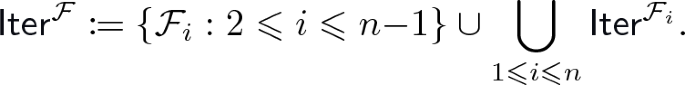
A $\mu$-forest of $u \in A^*$ can also be seen as “the word u with brackets” in definition 4.1. Therefore can be seen as a language over . In this setting, it is well-known that of bounded height can effectively be computed by a , i.e. a particular case of that can be computed by a non-deterministic one-way transducer (see e.g. [8]).

Theorem 4.2

(Simon [6, 19]). Given a morphism $\mu : A^* \rightarrow \mathbb {M}$ into a finite monoid $\mathbb {M}$, one can effectively build a such that for all $u \in A^*$, .

Building of bounded height is especially useful for us, since it enables to decompose any word in a somehow bounded way. This decomposition will be guided by the following definitions, that have been introduced in [8, 10]. First, we define as the middle children of .

Definition 4.3

Let . Its , denoted , are:

• if $\mathcal {F}= \langle a \rangle \in A$ or $\mathcal {F}= \varepsilon$, then ;

• otherwise if $\mathcal {F}= \langle \mathcal {F}_1, \cdots ,\mathcal {F}_n \rangle$, then:

  

Now, we define the notion of of a node $\mathfrak {t}$, which contains all the descendants of $\mathfrak {t}$ except those which are .

Definition 4.4

(Skeleton, frontier).

Let , , we define the of $\mathfrak {t}$, denoted , by:

• if $\mathfrak {t}= \langle a \rangle \in A$ is a leaf, then ;

• otherwise if $\mathfrak {t}= \langle \mathcal {F}_1, \cdots , \mathcal {F}_n \rangle$, then .

The of $\mathfrak {t}$ is the set containing the positions of u which belong to (when seen as leaves of the $\mathcal {F}$ over u).

Example 4.5

Let $\mathbb {M}{:}{=}(\{-1,1,0\}, \times )$ and $\mu : \mathbb {M}^* \rightarrow \mathbb {M}$ the product. A $\mathcal {F}$ of the word $(-1)(-1)0(-1)000000$ is depicted in Figure 4. Double lines denote . The set of blue nodes is the of the topmost blue node.

Fig. 4.

  and a .

It is easy to observe that for , the size of a , or of a , is bounded independently from $\mathcal {F}$. Furthermore, the set of is a partition of [8, Lemma 33]. As a consequence, the set of is a partition of [1 :  |u|]. Given a position $1 \leqslant i \leqslant |u|$, we can thus define the of i in $\mathcal {F}$, denoted , as the unique such that .

Definition 4.6

(Observation). Let and . We say that if either $\mathfrak {t}'$ is an ancestor of $\mathfrak {t}$, or $\mathfrak {t}'$ is the immediate right or left sibling of an ancestor of $\mathfrak {t}$.

Fig. 5.

Nodes that and that

The intuition behind the notion of (which is not symmetrical) is depicted in fig. 5. Note that in a forest of bounded height, the number of nodes that some $\mathfrak {t}$ is bounded. This will be a key argument in the following. We say that $\mathfrak {t}$ and $\mathfrak {t}'$ are if either $\mathfrak {t}$ $\mathfrak {t}'$ or the converse. Given $\mathcal {F}$, we can translate these notions to the positions of u: we say that i (resp. on) $i'$ if (resp. on) .

5 Height minimization of blind pebble transducers

In this section, we show theorem 3.5 for . We say that a $\mathscr {T}$ is a of a $\mathscr {B}$ if $\mathscr {T}$ labels a node in the tree description of $\mathscr {B}$. If $\mathscr {B}= \mathscr {T}\langle \mathscr {B}_1, \dots , \mathscr {B}_n \rangle$, we say that the $\mathscr {T}$ is the of $\mathscr {B}$. We let the of $\mathscr {B}$ be the cartesian product of all the of all the of $\mathscr {B}$. Observe that it makes sense to consider the of a $\mathscr {T}$ in a defined using the of $\mathscr {B}$.

5.1 Pumpability

We first give a sufficient condition, named , for a to compute a function f such that $|f(u)| \ne \mathcal {O}(|u|^{k-1})$. The behavior of a is depicted in fig. 6 over a well-chosen input: it has a factor in which the $\mathscr {T}_1$ calls a $\mathscr {T}_2$, and a factor in which $\mathscr {T}_2$ produces a non-empty output. Furthermore both factors can be iterated without destroying the runs of these machines (due to idempotents).

Definition 5.1

Let $\mathscr {B}$ be a whose is $\mu : A^* \rightarrow \mathbb {T}$. We say that the transducer $\mathscr {B}$ is if there exists:

• $\mathscr {T}_1, \dots , \mathscr {T}_k$ of $\mathscr {B}$, such that $\mathscr {T}_1$ is the of $\mathscr {B}$;

• $m_0, \dots , m_k, {\ell }_1, \dots , {\ell _k}, r_1, \dots , r_k \in \mu (A^*)$;

• $a_1,\dots , a_k \in A$ such that for all $1 \leqslant j \leqslant k$, $e_j {:}{=}{\ell }_j \mu (a_j) r_j$ is an idempotent;

• a permutation $\sigma : [{1}{:}{k}] \rightarrow [{1}{:}{k}]$;

such that if $\mathcal {M}_{i}^{j} {:}{=}m_{i} e_{i + 1} m_{i + 1} \cdots e_{j} m_{j}$ for all $0 \leqslant i \leqslant j \leqslant k$, and if we define the following for all $1 \leqslant j \leqslant k$:

$$\begin{aligned} \begin{aligned} \mathcal {C}_j {:}{=}\mathcal {M}_{0}^{\sigma (j)-1} e_{\sigma (j)} \ell _{\sigma (j)} {\boldsymbol{\llbracket } a_{\sigma (j)}\boldsymbol{\rrbracket }} r_{\sigma (j)} e_{\sigma (j)} \mathcal {M}_{\sigma (j)}^{k} \end{aligned} \end{aligned}$$

then for all $1 \leqslant j \leqslant k{-}1$, , and .

Fig. 6.

  in a .

Lemma 5.2 follows by choosing inverse images in $A^*$ for the $m_i$, $\ell _i$ and $r_i$.

Lemma 5.2

Let f be computed by a . There exists words $v_0, \dots , v_k, u_1, \dots , u_k$ such that $|f(v_0 u_1^{X} \cdots u_k^{X} v_k)| = \Theta (X^k)$.

Now, we use as a key ingredient for showing theorem 3.5, which directly follows by induction from the more precise theorem 5.3.

Theorem 5.3

(Removing one layer). Let $k \geqslant 2$ and $f : A^* \rightarrow B^*$ be computed by a $\mathscr {B}$. The following are equivalent:

• 1. $|f(u)| = \mathcal {O}(|u|^{k-1})$;

• 2. $\mathscr {B}$ is not ;

• 3. f can be computed by a .

Furthermore, this property is decidable and the construction is effective.

Proof

Item 3 $\Rightarrow$ item 1 is obvious. Item 1 $\Rightarrow$ item 2 is lemma 5.2. Furthermore, can be tested by an enumeration of $\mu (A^*)$ and A. It remains to show item 2 $\Rightarrow$ item 3 (in an effective fashion): this is the purpose of section 5.2.

5.2 Algorithm for removing a recursion layer

Let $k \geqslant 2$ and $\mathscr {U}$ be a that is not , and that computes $f : A^* \rightarrow B^*$. We build a $\overline{\mathscr {U}}$ for f.

Let $\mu : A^* \rightarrow \mathbb {T}$ be the of $\mathscr {U}$. We shall consider that, on input $u \in A^*$, the of $\overline{\mathscr {U}}$ can in fact use as input. Indeed is a (by theorem 4.2), hence its information can be recovered by using a . Informally, the feature enables a to chose its transitions not only depending on its current state and current letter u[i] in position $1 \leqslant i \leqslant |u|$, but also on a regular property of the prefix $u[1{:}i{-}1]$ and the suffix $u[i{+1}{:}|u|]$. It is well-known that given a $\mathscr {T}$ with , one can build an equivalent $\mathscr {T}'$ that does not have this feature (see e.g. [12, 15]). Furthermore, even if the accepting runs of $\mathscr {T}$ and $\mathscr {T}'$ may differ, they produce the same outputs from the same positions (this observation will be critical for , in order to ensure that the marked positions of the recursive calls will be preserved).

Now, we describe the that are the of $\overline{\mathscr {U}}$. First, it has for $\mathscr {T}$ a of $\mathscr {U}$, which are described in algorithm 1. Intuitively, is just a copy of $\mathscr {T}$. It is clear that if $\mathscr {T}$ is a of $\mathscr {U}$, then is the concatenation of the outputs produced by (the recursive calls of) $\mathscr {T}$ along its accepting run on .

$\overline{\mathscr {U}}$ also has for $\mathscr {T}$ a of $\mathscr {U}$, which are described in algorithm 2. Intuitively, simulates $\mathscr {T}$ while trying to inline recursive calls in its own run. More precisely, let $u \in A^*$ be the input and . If $\mathscr {T}$ calls $\mathscr {B}'$ in $1 \leqslant i \leqslant |u|$ that belongs to the of the root node $\mathcal {F}$ of $\mathcal {F}$, then inlines the behavior of the of $\mathscr {B}'$. Otherwise it makes a recursive call, except if $\mathscr {B}'$ is a leaf of $\mathscr {U}$. Hence if $\mathscr {T}$ is a of $\mathscr {U}$ which is not a leaf, is the concatenation of the outputs produced by the calls of $\mathscr {T}$ along its accepting run.

Finally, the transducer $\overline{\mathscr {U}}$ is obtained by defining to be its , where $\mathscr {T}$ is the of $\mathscr {U}$. Furthermore, we remove the or which are never called. Observe that $\overline{\mathscr {U}}$ indeed computes the function f. Furthermore, we observe that $\overline{\mathscr {U}}$ has recursion height (i.e. the number of nested Call instructions, plus 1 for the ) $k{-}1$, since each inlining of lines 9, 10 and 12 in algorithm 2 removes exactly one recursion layer of $\mathscr {U}$.

It remains to justify that each can be implemented by a (i.e. with but a bounded memory). We represent variable i by the current position of the transducer. Since it has access to $\mathcal {F}$, the can be used to check whether or not (since the size of is bounded). It remains to explain how the inlinings are performed:

• if , the inlines by executing the same moves and calls as $\mathscr {T}'$ does. Once its computation is ended, it has to go back to position i. This is indeed possible since belonging to is a property that can be detected by using the , hence the machine only needs to remember that i was the $\ell$-th position of ($\ell$ being bounded);

• else if $\mathscr {B}' = \mathscr {T}'$ is a , we produce the output of $\mathscr {T}'$ without moving. This is possible since for all , (hence the output of $\mathscr {T}'$ on u is bounded, and its value can be determined without moving, just by using the ). Indeed, if for such an when reaching line 12 of algorithm 2, then the conditions of lemma 5.4 hold, which yields a contradiction. This lemma is the key argument of this proof, relying on the non- of $\mathscr {U}$.

Lemma 5.4

(Key lemma). Let $u \in A^*$ and . Assume that there exists a sequence $\mathscr {T}_1, \dots , \mathscr {T}_k$ of of $\mathscr {U}$ and a sequence of positions $1 \leqslant i_1, \dots , i_k \leqslant |u|$ such that:

• $\mathscr {T}_1$ is the of $\mathscr {U}$;

• for all $1 \leqslant j \leqslant k{-}1$, and ;

• for all $1 \leqslant j \leqslant k$, (i.e. ).

Then $\mathscr {B}$ is .

Proof

(idea). We first observe that follows as soon as the nodes are pairwise . We then show that this condition can always be obtained, up to duplicating some subtrees of $\mathcal {F}$ (and some factors of u), because the behavior of a in a does not depend on the positions of the above recursive calls.

6 Height minimization of last pebble transducers

In this section, we show theorem 3.5 for . The notions of , and for a are defined as in section 5. The is now defined over .

6.1 Pumpability

The sketch of the proof is similar to section 5. We first give an equivalent of for . The intuition behind this notion is depicted in fig. 7. The formal definition is however more cumbersome, since we need to keep track of the fact that the calling position is marked.

Definition 6.1

Let $\mathscr {L}$ be a whose is $\mu : (A \cup \underline{A})^* \rightarrow \mathbb {T}$. We say that the transducer $\mathscr {L}$ is if there exists:

• $\mathscr {T}_1, \dots , \mathscr {T}_k$ of $\mathscr {L}$, such that $\mathscr {T}_1$ is the of $\mathscr {L}$;

• $m_0, \dots , m_k, {\ell }_1, \dots , {\ell _k}, r_1, \dots , r_k \in \mu (A^*)$;

• $a_1,\dots , a_k \in A$ such that for all $1 \leqslant j \leqslant k$, $e_j {:}{=}{\ell }_j \mu (a_j) r_j$ is idempotent;

• a permutation $\sigma : [{1}{:}{k}] \rightarrow [{1}{:}{k}]$;

such that if we let $\mathcal {M}_{i}^{j} {:}{=}m_{i} e_{i + 1} m_{i + 1} \cdots e_{j} m_{j}$ for all $0 \leqslant i \leqslant j \leqslant k$, and if we define the following :

and for all $1 \leqslant j \leqslant k{-}1$ the :

then for all $1 \leqslant j \leqslant k{-}1$, , and .

Fig. 7.

  in a .

We obtain lemma 6.2 by a proof which is similar to that of lemma 5.2.

Lemma 6.2

Let f be computed by a . There exists words $v_0, \dots , v_k, u_1, \dots , u_k$ such that $|f(v_0 u_1^{X} \cdots u_k^{X} v_k)| = \Theta (X^k)$.

Theorem 6.3

(Removing one layer). Let $k \geqslant 2$ and $f : A^* \rightarrow B^*$ be computed by a $\mathscr {L}$. The following are equivalent:

• 1. $|f(u)| = \mathcal {O}(|u|^{k-1})$;

• 2. $\mathscr {L}$ is not ;

• 3. f can be computed by a .

Furthermore, this property is decidable and the construction is effective.

Proof

Item 3 $\Rightarrow$ item 1 is obvious. Item 1 $\Rightarrow$ item 2 is lemma 6.2. Furthermore, can be tested by an enumeration of $\mu (A^*)$ and A. It remains to show item 2 $\Rightarrow$ item 3 (in an effective fashion): this is the purpose of section 6.2.

6.2 Algorithm for removing a recursion layer

Let $k \geqslant 2$ and $\mathscr {U}$ be a that is not , and that computes $f : A^* \rightarrow B^*$. We build a $\overline{\mathscr {U}}$ for f. Let be the of $\mathscr {U}$. As before (using a ), the of $\overline{\mathscr {U}}$ have access to on input $u \in A^*$.

Now, we describe the of $\overline{\mathscr {U}}$. It has for $\mathscr {T}$ a of $\mathscr {U}$ and $\rho$ a run of $\mathscr {T}$, which are described in algorithm 1. Intuitively, these machines mimics the behavior of $\mathscr {T}$ along the run $\rho$ (which is not necessarily accepting) of $\mathscr {T}$ over with .

Since they are indexed by a run $\rho$, it may seem that we create an infinite number of , but it will not be the case. Indeed, a run $\rho$ will be represented by its first configuration $(q_1,i_1)$ and last configuration $(q_n,i_n)$. This information is sufficient to simulate exactly the two-way moves of $\rho$, but there is still an unbounded information: the positions $i_1$ and $i_n$. In fact, the input will be of the form and we shall guarantee that the $i_1$ and $i_n$ can be detected by the if i is marked. Hence the run $\rho$ will be represented in a bounded way, independently from the input v, and so that its first and last configurations can be detected by the of the .

It follows from algorithm 3 that if $\mathscr {T}$ is a of $\mathscr {U}$, then for all $v \in (A \cup \underline{A})^*$ and $\rho$ run of $\mathscr {T}$ on , is the concatenation of the outputs produced by (the recursive calls of) $\mathscr {T}$ along $\rho$.

We also define a that is similar to , except that it ignores the mark of its input and acts as if it was in position i (as above for $\rho$, i will be encoded by a bounded information).

$\overline{\mathscr {U}}$ also has for $\mathscr {T}$ a of $\mathscr {U}$, which are described in algorithm 4. Intuitively, simulates $\mathscr {T}$ along $\rho$ while trying to inline some recursive calls. Whenever it is in position i and needs to call recursively $\mathscr {L}'$ whose is $\mathscr {T}'$, it first the accepting run $\rho '$ of $\mathscr {T}'$ on , with respect to and i, as explained in definition 6.4 and depicted in fig. 8. Intuitively, this operation splits $\rho '$ into a bounded number of runs whose positions either all i, or i all of them, or none of these cases occur (the positions are either 0, $|u|{+}1$ or of i).

Definition 6.4

(Slicing). Let $u \in A^*$, and $1 \leqslant i \leqslant |u|$. We let (resp. ) be the set of positions that i (resp. that i).

Let be a run of a $\mathscr {T}$ on . We build by induction a sequence $\ell _1, \dots , \ell _{N+1}$ with $\ell _1 {:}{=}1$ and:

• if $\ell _j = n {+} 1$ then $j {:}{=}N$ and the process ends;

• else if (resp. , resp. ), then $\ell _{j+1}$ is the largest index such that for all $\ell _{j} \leqslant \ell \leqslant \ell _{j+1}{-}1$, (resp. , resp. ).

Finally the of $\rho$ ,with respect to $\mathcal {F}$ and i, is the sequence of runs $\rho _1, \dots , \rho _{N}$ where .

Fig. 8.

  of a run $\rho$ with respect to i and $\mathcal {F}$.

Now, let $\rho '_1, \dots , \rho '_N$ be of the run $\rho '$ of $\mathscr {T}'$ on the input . For all $1 \leqslant j \leqslant N$, there are mainly two cases. Either the positions of $\rho '_j$ all are in or . In this case, directly inlines within its own run (i.e. without making a recursive call). Otherwise, it makes a recursive call to , except if $\mathscr {L}'$ is a leaf of $\mathscr {U}$ (thus $\mathscr {L}' = \mathscr {T}'$).

Finally, $\overline{\mathscr {U}}$ is described as follows: on input $u \in A^*$, its is the , where $\mathscr {T}$ is the of $\mathscr {U}$ and $\rho$ is the accepting run of $\mathscr {T}$ on (represented by the bounded information that it is both initial and final). As before, we remove the which are never called in $\overline{\mathscr {U}}$. Observe that we have created a machine with recursion height $k{-}1$ (because line 17 in algorithm 4 prevents from calling a k-th layer).

Let us justify that each can indeed be implemented by a . First, let us observe that since $\mathcal {F}$ has bounded height, the number N of given in line 7 of algorithm 4 is bounded. Furthermore, we claim that the first and last positions of each $\rho '_j$ belong to a given set of bounded size, which can be detected by a which has access to i. For the $\rho '_j$ whose positions are in , this is clear since is bounded (because the frontier of any node is bounded). For we use lemma 6.5, which implies that this set is a bounded union of intervals. The last case is very similar.

Lemma 6.5

Let $1 \leqslant i \leqslant |u|$, and $\mathfrak {t}_{1}$ (resp. $\mathfrak {t}_2$) be its immediate left (resp. right) sibling (they exist whenever , i.e. here $\mathfrak {t}\ne \mathcal {F}$). Then:

This analysis justifies why each $\rho '_j$ can be encoded in a bounded way. Now, we show how to implement the inlinings while using i as the current position:

• if , then n is bounded (because is bounded). We can thus inline while staying in position i. However, when $\mathscr {T}'$ calls some $\mathscr {L}''$ (of $\mathscr {T}''$) on position $i_{\ell }$, we would need to call (where $\rho ''$ is the accepting run of $\mathscr {T}''$ along ). But we cannot do this operation, since we are in position i and not in $i_{\ell }$. The solution is that the inlined code calls instead, which simulates an accepting run $\rho ''$ of $\mathscr {T}$ on , even if its input is . Note that $i_{\ell }$ can be represented as a bounded information and recovered by a given as input, since i $i_{\ell }$;

• if , then the nodes are roughly below in $\mathcal {F}$ (see fig. 5). We inline , by moving along $i_1, \dots , i_n$ as $\rho '_j$ does. We can keep track of the height of above the current (it is a bounded information). With the , we can detect the end of $\rho '_j$, and go back to position i.

It remains to justify that $\overline{\mathscr {U}}$ is correct. For this, we only need to show that when it reaches line 18 in algorithm 4, the output of $\mathscr {T}'$ along $\rho '_j$ is indeed empty. Otherwise, the conditions of lemma 6.6 would hold (since we never execute two successive recursive calls in positions). It provides a contradiction.

Lemma 6.6

(Key lemma). Let $u \in A^*$ and . Assume that there exists a sequence $\mathscr {T}_1, \dots , \mathscr {T}_k$ of of $\mathscr {U}$ and a sequence of positions $1 \leqslant i_1, \dots , i_k \leqslant |u|$ such that:

• $\mathscr {T}_1$ is the of $\mathscr {U}$;

• and ;

• for all $2 \leqslant j \leqslant k{-}1$, ;

• for all $1 \leqslant j \leqslant k{-}1$, and are ;

Then $\mathscr {U}$ is .

Proof

(idea). As for lemma 5.4, the key observation is that follows as soon as the nodes are pairwise . Furthermore, this condition can be obtained by duplicating some nodes in $\mathcal {F}$.

7 Making the two last pebbles visible

We can define a similar model to that of , which sees the two last calling positions instead of only the previous one. Let us name this model a . A very natural question is to know whether we can show an analog of theorem 3.5 for these machines.

Note that for $k=1,2$ and 3, a is exactly the same as a . Hence the function of page 2 is such that and can be computed by a , but it cannot be computed by a . It follows that the connection between minimal recursion height and growth of the output fails. However, this result is somehow artificial. Indeed, a is a degenerate case, since it can only see one last pebble. More interestingly, we show that the connection fails for arbitrary heights.

Theorem 7.1

For all $k \geqslant 2$, there exists a function $f:A^* \rightarrow B^*$ such that $|f(u)| = \mathcal {O}(|u|^2)$ and that can be computed by a , but not by a .

Proof

(idea). We re-use a counterexample introduced by Bojańczyk in [2] to show a similar failure result for the model of .

8 Outlook

This paper somehow settles the discussion concerning the variants of for which the minimal recursion height only depends on the growth of the output. As soon as two marks are visible, the combinatorics of the output also has to be taken into account, hence minimizing the recursion height in this case (e.g. for ) seems hard with the current tools.

As observed in [13], one can extend by allowing the recursion height to be unbounded (in the spirit of [9]). This model enables to produce outputs whose size grows exponentially in the size of the input. A natural question is to know whether a function computed by this model, but whose output size is polynomial, can in fact be computed with a recursion stack of bounded height (i.e. by a ).

References

Bojańczyk, M.: Polyregular functions. arXiv preprint arXiv:1810.08760 (2018)
Bojańczyk, M.: The growth rate of polyregular functions. arXiv preprint arXiv:2212.11631 (2022)
Bojańczyk, M.: Transducers of polynomial growth. In: Proceedings of the 37th Annual ACM/IEEE Symposium on Logic in Computer Science. pp. 1–27 (2022)
Bojańczyk, M., Kiefer, S., Lhote, N.: String-to-string interpretations with polynomial-size output. In: 46th International Colloquium on Automata, Languages, and Programming, ICALP 2019 (2019)
Chytil, M.P., Jákl, V.: Serial composition of 2-way finite-state transducers and simple programs on strings. In: 4th International Colloquium on Automata, Languages, and Programming, ICALP 1977. pp. 135–147. Springer (1977)
Colcombet, T.: Green’s relations and their use in automata theory. In: International Conference on Language and Automata Theory and Applications. pp. 1–21. Springer (2011)
Dave, V., Gastin, P., Krishna, S.N.: Regular transducer expressions for regular transformations. In: Proceedings of the 33rd Annual ACM/IEEE Symposium on Logic in Computer Science. pp. 315–324. ACM (2018)
Douéneau-Tabot, G.: Pebble transducers with unary output. In: 46th International Symposium on Mathematical Foundations of Computer Science, MFCS 2021 (2021)
Douéneau-Tabot, G., Filiot, E., Gastin, P.: Register transducers are marble transducers. In: 45th International Symposium on Mathematical Foundations of Computer Science, MFCS 2020 (2020)
Douéneau-Tabot, G.: Hiding pebbles when the output alphabet is unary. In: 49th International Colloquium on Automata, Languages, and Programming, ICALP 2022 (2022)
Engelfriet, J.: Two-way pebble transducers for partial functions and their composition. Acta Informatica 52(7-8), 559–571 (2015)
Engelfriet, J., Hoogeboom, H.J.: MSO definable string transductions and two-way finite-state transducers. ACM Transactions on Computational Logic (TOCL) 2(2), 216–254 (2001)
Engelfriet, J., Hoogeboom, H.J., Samwel, B.: Xml transformation by tree-walking transducers with invisible pebbles. In: Proceedings of the twenty-sixth ACM SIGMOD-SIGACT-SIGART symposium on Principles of database systems. pp. 63–72.ACM (2007)
Gurari, E.M.: The equivalence problem for deterministic two-way sequential transducers is decidable. SIAM Journal on Computing 11(3), 448–452 (1982)
Hopcroft, J.E., Ullman, J.D.: An approach to a unified theory of automata. The Bell System Technical Journal 46(8), 1793–1829 (1967)
Kiefer, S., Nguyên, L.T.D., Pradic, C.: Revisiting the growth of polyregular functions: output languages, weighted automata and unary inputs. arXiv preprint arXiv:2301.09234 (2023)
Nguyên, L.T.D., Noûs, C., Pradic, C.: Comparison-free polyregular functions. In: 48th International Colloquium on Automata, Languages, and Programming, ICALP 2021 (2021)
Shepherdson, J.C.: The reduction of two-way automata to one-way automata. IBM Journal of Research and Development 3(2), 198–200 (1959)
Simon, I.: Factorization forests of finite height. Theor. Comput. Sci. 72(1), 65–94 (1990)
Acknowledgements
The author is grateful to Tito Nguyên for suggesting the study of the recursion height for
.
Author information
Authors and Affiliations
Corresponding author
Editor information
Editors and Affiliations
Rights and permissions
Open Access This chapter is licensed under the terms of the Creative Commons Attribution 4.0 International License (http://creativecommons.org/licenses/by/4.0/), which permits use, sharing, adaptation, distribution and reproduction in any medium or format, as long as you give appropriate credit to the original author(s) and the source, provide a link to the Creative Commons license and indicate if changes were made.
The images or other third party material in this chapter are included in the chapter's Creative Commons license, unless indicated otherwise in a credit line to the material. If material is not included in the chapter's Creative Commons license and your intended use is not permitted by statutory regulation or exceeds the permitted use, you will need to obtain permission directly from the copyright holder.
Copyright information
© 2023 The Author(s)
About this paper
Cite this paper
Douéneau-Tabot, G. (2023). Pebble minimization: the last theorems. In: Kupferman, O., Sobocinski, P. (eds) Foundations of Software Science and Computation Structures. FoSSaCS 2023. Lecture Notes in Computer Science, vol 13992. Springer, Cham. https://doi.org/10.1007/978-3-031-30829-1_21
Download citation
DOI: https://doi.org/10.1007/978-3-031-30829-1_21
Published:
Publisher Name: Springer, Cham
Print ISBN: 978-3-031-30828-4
Online ISBN: 978-3-031-30829-1
eBook Packages: Computer ScienceComputer Science (R0)