The Well-Ordered Newtonian Mechanics

Abstract

Just like many scientific giants, Issac Newton (1643–1727) was also a weirdo. He was anti-social and aggressive, unique in thinking as well as actions, at the same time refusing to yield to authority. Born in the county of Lincolnshire, he later moved to Cambridge and London for research and government work, all the while living in his isolated world both mentally and physically, almost without any contact with real people, not to mention getting married. Though he spent his whole life in the long, narrow area bounded by these three places and never actually saw the ocean with his own eyes, he was able to describe the tidal phenomenon and its causing factors. Even more surprising, though, was how healthy he was. In fact, rumor has it that he only shed one single tooth from cradle to grave. Equally amazing was how he managed by integrating astronomy, physics, and mathematics in an unprecedented way to explain a number of celestial and earthly movements with physical concepts and calculate changes in the natural world with mathematical approaches, thereby solving certain astronomical mysteries that had perplexed natural philosopher for more than 2,000 years. With achievements that almost no one in the history of physics could ever emulate, he debunked Aristotle’s scientific hypothesis, which had been widely accepted for thousands of years and was still wielding significant influence on many scientists even in the 17th century. It’s no wonder the famous economist John Maynard Keynes (1883–1946) hailed him not only as a magician who bridged the gap between ancient natural philosophy and modern physics but also a model in present-day scientific research worthy of our tremendous respect.

萬有是如此簡約

引力是這般和諧

啊!萬有的引力

因有你

這個世界變得井然有序

我們也安然悠游於反覆更新的變化中

So harmonic is the universe

And so simple is the gravity

Ah, it’s all thanks to the universal gravitation

The world thus becomes an orderly space

And the universe reaches eternal through inertia and conservation

Appendices

Appendix 4.1: Calculating the Period of Earth’s Precession with the Law of Universal Gravity

Since the Earth is an oblate spheroid with slight bulges in the equatorial area, the gravitational forces of the Sun and Moon would each generate a torque on it and affect the angular momentum of its rotation. Meanwhile, the Earth works like a giant top that not just rotates but also revolves slowly with its axis forming a 23.5-degree angle with the ecliptic plane. This phenomenon, as demonstrated in Fig. 4.8, is called axial precession in mechanics, also called the precession of equinoxes in astronomy.

Fig. 4.8

The axial precession of the precession of equinoxes of the Earth

To determine the period of Earth’s precession, let’s first suppose there are two astronomical bodies whose masses are M and m, as shown in Fig. 4.9. If we set the origin of the xyz coordinate system at the barycenter of m, the center of M would fall on the x axis with a position vector of $\overset{\lower0.5em\hbox{$\smash{\scriptscriptstyle\rightharpoonup}$}} {R} = \left( {R,0,0} \right)$. Now, let’s again suppose there’s a small point mass dm in m whose position vector is $\overset{\lower0.5em\hbox{$\smash{\scriptscriptstyle\rightharpoonup}$}} {r} = \left( {x,y,z} \right)$ and forms the angle $\beta$ with $\overset{\lower0.5em\hbox{$\smash{\scriptscriptstyle\rightharpoonup}$}} {R}$. Considering that r, the average radius of m is far smaller than R, the distance between the two astronomical bodies, their combined gravitational energy can be represented as:

Fig. 4.9

The relationship between the two astronomical bodies to determine the period of the Earth’s precession

$$\begin{aligned} V & = - \int {\frac{GMdm}{{\sqrt {R^{2} + r^{2} - 2Rr\cos \beta } }}} \\ & \approx - \frac{GMm}{R} - \frac{GM}{{2R^{3} }}\int {r^{2} \left( {3\cos^{2} \beta - 1} \right)} dm \\ & = - \frac{GMm}{R} - \frac{GM}{{2R^{3} }}\int {\left( {2x^{2} - y^{2} - z^{2} } \right)} dm \\ \end{aligned}$$

(4.36)

Just like the Earth, as you can see in Fig. 4.9, m is also an oblate spheroid in this proposition and rotates on its axis of symmetry $z^{\prime}$. If we represent the moments of inertia from m’s circling on $z^{\prime}$ and $x^{\prime}$ as C and A respectively, we can confirm that $C > A$ because m is flat and oblong in shape while $z^{\prime}$ is its axis of rotation. Now, if we rotate the coordinate system by an angle of $(\pi /2) - \theta$ along the y-axis, $z^{\prime}$ still stays on the xz plane but will form the angle $\theta$ with the x-axis. Please note, that the post-rotation variant $y^{\prime}$ still points toward the paper and will overlap with the original y-axis. Meanwhile, the spin of the coordinate system would help us derive the equations below:

$$x = x^{\prime}\sin \theta + z^{\prime}\cos \theta ,$$

(4.37a)

$$z = - x^{\prime}\cos \theta + z^{\prime}\sin \theta$$

(4.37b)

Then, by substituting $x^{\prime},y^{\prime},{\text{and}}\,z^{\prime}$ for $x, y,{\text{and}}\,z$ in (4.36) with (4.37a) and (4.37b), we’ll come to the result below:

$$\begin{aligned} V & \approx - \frac{{GMm}}{R} \\ & \quad - \frac{{GM}}{{2R^{3} }}\int {\left[ \begin{aligned} & \left( {2\sin ^{2} \theta - \cos ^{2} \theta } \right)x^{{{\text{'}}2}} - y^{{{\text{'}}2}} + \left( {2\cos ^{2} \theta - \sin ^{2} \theta } \right)z^{{{\text{'}}2}} \\ &\quad + 6x^{\prime}z^{\prime}\sin \theta \cos \theta \hfill \\ \end{aligned} \right]dm} \\ \end{aligned}$$

(4.38)

Due to the symmetry of $x^{\prime}$ and $z^{\prime}$, the result of integrating the last item in (4.38), which contains $x^{\prime}z^{\prime}$, over m would be 0. Therefore, just a little simplification of the items of trigonometric functions in the above equation can help us rewrite it as:

$$V \approx - \frac{GMm}{R} - \frac{GM}{{2R^{3} }}\int {\left[ {\left( {1 - 3\cos^{2} \theta } \right)\left( {x^{\prime 2} - z^{\prime 2} } \right) - y^{\prime 2} + x^{\prime 2} } \right]} dm$$

(4.39)

In the meantime, we know of the two equations below because of the definition of the moment of inertia:

$$C = \int {\left( {x^{\prime 2} + y^{\prime 2} } \right)} dm,$$

(4.40a)

$$A = \int {\left( {y^{\prime 2} + z^{\prime 2} } \right)} dm = \int {\left( {x^{\prime 2} + z^{\prime 2} } \right)} dm$$

(4.40b)

Derived from Eq. (4.40a) and (4.40b) is (4.41):

$$\int {\left( {x^{{{\prime }2}} - z^{{{\prime }2}} } \right)dm} = C - A$$

(4.41)

While the symmetry mentioned before gives us (4.42):

$$\int {\left( { - y^{{{\prime }2}} + x^{{{\prime }2}} } \right)dm} = 0$$

(4.42)

Then, the substitution of (4.41), (4.42) into (4.39) would yield:

$$V \approx - \frac{GMm}{R} - \frac{GM}{{2R^{3} }}\left( {1 - 3\cos^{2} \theta } \right)\left( {C - A} \right)$$

(4.43)

To calculate the torque generated by M on m, we can differentiate the potential energy V over $\theta$ in (4.43):

$$\tau \approx - \frac{\partial V}{\partial \theta } = \frac{3GM}{{R^{3} }}\left( {C - A} \right)\sin \theta \cos \theta$$

(4.44)

From (4.44), we can see that the torque gives the angle $\theta$ a tendency to approach $\pi /2$. In other words, $z^{\prime}$ will slowly deviate towards z, meaning the direction of the torque points to $- y$.

While Earth’s axial precession is affected by the gravity of both Sun and Moon, here, let’s suppose the interaction between the two bodies is small enough to be disregarded, which is why we can evaluate the influence of each separately. If we follow the approach demonstrated above, the equations that are derived should be the same for both Sun and Moon; as long as we substitute two different sets of values as the parameters into the equations, we should be able to determine how the two bodies impact Earth’s precession. So, let’s first consider a system consisted only of the Sun and Earth, as shown in Fig. 4.10. If the z-axis is perpendicular to Earth’s revolving plane (i.e. the ecliptic plane), then its axis of rotation (ON) would always form the angle $\varphi$ with z. Then, if we again suppose the unit vector along ON is $\hat{n}$ and set its origin at point O, as time progresses, N will start motioning along the circle C continuously, as you can find illustrated in Fig. 4.10. In the next step, we need to mark a point (A) on C that would make $\overset{\lower0.5em\hbox{$\smash{\scriptscriptstyle\rightharpoonup}$}}{CA}$ parallel with $\hat{x}$ (the unit vector on the direction of x) and represent the angle $\angle NCA$ as $\alpha$.

Fig. 4.10

A schematic description to determine how the two bodies impact the Earth’s precession

Now, let’s look at a rotating coordinate system centered on the Sun where its angular velocity is equal to that of Earth’s revolution. While the centers of both bodies are in a stationary state, the Earth would, due to is a revolution, be affected by a centrifugal force that’s proportional to its revolving radius and points away from Sun. However, no net torque would be generated since centrifugal forces on Earth are always symmetric, yet when it comes to the Sun’s torque on Earth, it’s a varying value due to the continued circling of Earth’s rotation axis around z, which causes the angle $\alpha$ to be changing constantly. Therefore, we need to develop the mathematical relationship between this torque and $\alpha$ and calculate the integral of $\alpha$ to determine the result of $\left\langle {\cos^{2} \alpha } \right\rangle = \frac{1}{2}$, which is the average value of the torque. Please note that it is the direction of $\hat{x} \times \hat{n}$ that the torque points to. If we represent the angle between ON and the x-axis as $\theta$, then we can also use (4.44) to calculate the torque value, which can eventually be written as:

$$\overset{\lower0.5em\hbox{$\smash{\scriptscriptstyle\rightharpoonup}$}} {\tau } = \frac{3GM}{{R^{3} }}\left( {C - A} \right)\sin \theta \cos \theta \frac{{\hat{x} \times \hat{n}}}{{\left| {\hat{x} \times \hat{n}} \right|}}$$

(4.45)

As the angular momentum of Earth’s rotation points to the direction of $\hat{n}$, the direction along which the momentum changes (i.e. the direction of the torque) should be perpendicular to the plane defined by the points O, C, and N, which can also be understood as the direction of $\hat{e} = \left( {\sin \alpha , - \cos \alpha ,0} \right)$. Therefore, it’s only the torque on the direction of $\hat{e}$, which can be represented as $\overset{\lower0.5em\hbox{$\smash{\scriptscriptstyle\rightharpoonup}$}} {\tau } \cdot \hat{e}$, that contributes effectively to the precession of Earth. As for torques that point to other directions, they do cause $\varphi$, the angle between the axis of rotation and z-axis to change, but only to so small of a degree that the influence can be disregarded in this proposition.

Now, we can substitute all the angles and vectors in Eq. (4.45) with equations of $\varphi$ and $\theta$. Since related vectors $\hat{x}$ and $\hat{n}$ can be written as $\left( {1,0,0} \right)$ and $\left( {\sin \varphi \cos \alpha ,\sin \varphi \sin \alpha ,\cos \varphi } \right)$ respectively, we can derive $\cos \theta = \hat{n} \cdot \hat{x} = \sin \varphi \cos \alpha$, which leads us to the equation of the effective torque, as shown below:

$$\begin{aligned} \overset{\lower0.5em\hbox{$\smash{\scriptscriptstyle\rightharpoonup}$}} {\tau } \cdot \hat{e} & = \frac{3GM}{{R^{3} }}\left( {C - A} \right)\sin \theta \cos \theta \frac{{\hat{x} \times \hat{n}}}{{\left| {\hat{x} \times \hat{n}} \right|}} \cdot \hat{e} \\ & = \frac{3GM}{{R^{3} }}\left( {C - A} \right)\sqrt {1 - \sin^{2} \varphi \cos^{2} \alpha } \sin \varphi \cos \alpha \\ & \quad \frac{{\left( {0, - \cos \varphi ,\sin \varphi \sin \alpha } \right)}}{{\sqrt {\cos^{2} \varphi + \sin^{2} \varphi \sin^{2} \alpha } }} \cdot \left( {\sin \alpha , - \cos \alpha ,0} \right) \\ & = \frac{3GM}{{R^{3} }}\left( {C - A} \right)\sqrt {1 - \sin^{2} \varphi \cos^{2} \alpha } \sin \varphi \cos \alpha \frac{\cos \varphi \cos \alpha }{{\sqrt {1 - \sin^{2} \varphi \cos^{2} \alpha } }} \\ & = \frac{3GM}{{R^{3} }}\left( {C - A} \right)\sin \varphi \cos \varphi \cos^{2} \alpha \\ \end{aligned}$$

(4.46)

After integrating the parameter $\alpha$ in (4.46) and adopting the average, we can derive:

$$\left\langle {\overset{\lower0.5em\hbox{$\smash{\scriptscriptstyle\rightharpoonup}$}} {\tau } \cdot \hat{e}} \right\rangle = \frac{3GM}{{2R^{3} }}\left( {C - A} \right)\sin \varphi \cos \varphi$$

(4.47)

Please, note that $\left\langle {\cos^{2} \alpha } \right\rangle = \frac{1}{2}$ was used in the derivation process above. Therefore, (4.47) is exactly the effective torque generated by the Sun (or Moon) on Earth.

Then, as the angular momentum of Earth’s rotation is $\overset{\lower0.5em\hbox{$\smash{\scriptscriptstyle\rightharpoonup}$}} {L} = C\omega \hat{n}$, where $\omega$ is the angular velocity of its rotating movement, we can again derive the below equation:

$$\frac{d}{dt}\overset{\lower0.5em\hbox{$\smash{\scriptscriptstyle\rightharpoonup}$}} {L} = \left( {\overset{\lower0.5em\hbox{$\smash{\scriptscriptstyle\rightharpoonup}$}} {\tau } \cdot \hat{e}} \right)\hat{e}$$

(4.48)

As a result, the angular velocity of Earth’s axial precession can be written as:

$$\frac{d\alpha }{dt} = - \frac{3GM}{{2R^{3} }}\left( {\frac{C - A}{C}} \right)\frac{\cos \varphi }{\omega }$$

(4.49)

Note: In (4.49), the negative signifier means the precession is clock-wise if we look down from the top of $\hat{z}$-axis.

One thing that should be noted here is that the gravity causing Earth’s axial precession comes from both Sun and Moon, and the total amount of torque also consists of the torques generated separately by the two bodies. Similarly, the total angular velocity of precession exerted by the Sun and Moon on Earth’s axis of rotation is also the combination of their respective effects. Therefore, we need to calculate the angular velocity given by each with Eq. (4.49) and add up the results. To do so, we’ll need to substitute the following values:

$$\begin{aligned} \varphi & = 23.5^\circ ,G = 6.67 \times 10^{ - 11} \;{\text{m}}^{3} \;{\text{kg}}^{ - 1} \;{\text{s}}^{ - 2} ,\left[ {\frac{C - A}{C}} \right]{\text{of Earth}} \\ & = 0.003273763 \end{aligned}$$

(4.50)

The mass of Sun $M_{s} = 1.989 \times 10^{30} \,{\text{kg}}$, the mass of Moon $M_{m} = 7.36 \times 10^{22} \,{\text{kg}}$, the average distance between Sun and Earth $R_{s} = 1.496 \times 10^{11} \,{\text{m}}$, and the average distance between Moon anFVVd Earth $R_{m} = 3.844 \times 10^{8} \,{\text{m}}$. In the end, the period of Earth’s axial precession can be calculated to be:

$$2\pi \left[ {\frac{3G}{2}\left( {\frac{C - A}{C}} \right)\frac{\cos \varphi }{\omega }\left( {\frac{{M_{s} }}{{R_{s}^{3} }} + \frac{{M_{m} }}{{R_{m}^{3} }}} \right)} \right]^{ - 1} \approx 25,500({\text{years}})$$

(4.51)

As the result is only 300 years apart from the actual value, which is 25,800 years, we can safely assume that our derivation process is quite accurate.

Appendix 4.2: Measuring the Influence of Moon’s Gravity on Earth Tides with the Law of Universal Gravitation

The mathematical derivation and the two figures of this proposition are referred to Zhao and Jiao [35] as well as Chap. 10 of Morin [24].

This proposition demonstrates how we can analyze the influence of lunar gravity on Earth’s tidal movements with the law of universal gravity. As shown in Fig. 4.11, in a rotating reference frame where the center of mass of the moon and earth sits at the center, the effective force working on the oceans on Earth is the sum of Moon’s gravity and the centrifugal force arising from the inertia of the Moon-Earth co-orbiting. If you look at Fig. 4.11, you can see the distribution of this effective force, which draws the seawater on Earth along the direction of the line joining the two bodies and shapes the Earth into an ellipse. As illustrated below, the highest points of the two tidal bulges both sit on the same line mentioned above, which explains why locations that are 180° apart in longitude would see simultaneous tides and contribute to the phenomenon of double day tide.

Fig. 4.11

A schematic description of the tide of the Earth-Moon system. Referenced from Fig. 3 of Zhao and Jiao [35]

In Fig. 4.11, G is the gravitational constant, $M_{m}$ the mass of Moon, C/C’ the center of Moon/Earth, P the height of seawater, whose mass is $\Delta m$, $\left| {\overset{\lower0.5em\hbox{$\smash{\scriptscriptstyle\rightharpoonup}$}}{r\prime } } \right|$ the distance from P to the Moon’s barycenter $\left( { = \sqrt {r^{2} + R^{2} - 2rR\cos \theta } = r\prime } \right)$, and $\left| {\overset{\lower0.5em\hbox{$\smash{\scriptscriptstyle\rightharpoonup}$}} {R} } \right|$ the distance from P to the center of Earth $\left( { = \left| {\overset{\lower0.5em\hbox{$\smash{\scriptscriptstyle\rightharpoonup}$}}{CP} } \right| = R} \right)$. As for the distance between the centers of Moon and Earth, it can be represented as $\left| {\overset{\lower0.5em\hbox{$\smash{\scriptscriptstyle\rightharpoonup}$}} {r} } \right| = \left| {\overset{\lower0.5em\hbox{$\smash{\scriptscriptstyle\rightharpoonup}$}}{CC\prime } } \right| = r$. To start the derivation process, let’s first use the following equation to represent the lunar gravity exerted on $\Delta m$, the seawater on Earth:

$$\overset{\lower0.5em\hbox{$\smash{\scriptscriptstyle\rightharpoonup}$}} {f} = \frac{{G\Delta mM_{m} }}{{r^{\prime 3} }}\overset{\lower0.5em\hbox{$\smash{\scriptscriptstyle\rightharpoonup}$}}{{r^{\prime } }}$$

(4.52)

On the other hand, the seawater is also acted upon by a centrifugal force that arises from inertia:

$$\vec{f}_{I} = - \frac{{G\Delta mM_{m} }}{{r^{3} }}\overset{\lower0.5em\hbox{$\smash{\scriptscriptstyle\rightharpoonup}$}} {r}$$

(4.53)

Therefore, we know the Moon’s tidal drawing force on Earth’s oceans should be the sum of (4.52) and (4.53):

$$\vec{f}_{T} = \overset{\lower0.5em\hbox{$\smash{\scriptscriptstyle\rightharpoonup}$}} {f} + \vec{f}_{I} = G\Delta mM_{m} \left( {\frac{{\overset{\lower0.5em\hbox{$\smash{\scriptscriptstyle\rightharpoonup}$}}{{r^{\prime}}} }}{{r^{\prime 3} }} - \frac{{\overset{\lower0.5em\hbox{$\smash{\scriptscriptstyle\rightharpoonup}$}} {r} }}{{r^{3} }}} \right) = G\Delta mM_{m} \left( {\frac{{\overset{\lower0.5em\hbox{$\smash{\scriptscriptstyle\rightharpoonup}$}} {r} - \overset{\lower0.5em\hbox{$\smash{\scriptscriptstyle\rightharpoonup}$}} {R} }}{{\left| {\overset{\lower0.5em\hbox{$\smash{\scriptscriptstyle\rightharpoonup}$}} {r} - \overset{\lower0.5em\hbox{$\smash{\scriptscriptstyle\rightharpoonup}$}} {R} } \right|^{3} }} - \frac{{\overset{\lower0.5em\hbox{$\smash{\scriptscriptstyle\rightharpoonup}$}} {r} }}{{r^{3} }}} \right)$$

(4.54)

Then, we can derive this equation below based on the geometrical properties observed from Fig. 4.11:

$$\left( {\overset{\lower0.5em\hbox{$\smash{\scriptscriptstyle\rightharpoonup}$}} {r} - \overset{\lower0.5em\hbox{$\smash{\scriptscriptstyle\rightharpoonup}$}} {R} } \right)_{x} = r - R\cos \theta ,$$

(4.55a)

$$\left( {\overset{\lower0.5em\hbox{$\smash{\scriptscriptstyle\rightharpoonup}$}} {r} - \overset{\lower0.5em\hbox{$\smash{\scriptscriptstyle\rightharpoonup}$}} {R} } \right)_{y} = - R\sin \theta$$

(4.55b)

Now, let’s represent the horizontal (or x) and vertical (or y) components of the tidal drawing force $\vec{f}_{T}$ as $\left( {\vec{f}_{T} } \right)_{x}$ and $\left( {\vec{f}_{T} } \right)_{y}$ before simplifying the equations below by only considering the linear term of the lowest order when calculating $\frac{R}{r}$. In the end, we can obtain the approximate values of $\left( {\vec{f}_{T} } \right)_{x}$ and $\left( {\vec{f}_{T} } \right)_{y}$ as:

$$\left( {f_{T} } \right)_{x} = \frac{{G\Delta mM_{m} }}{{r^{2} }}\left[ {\frac{{1 - \frac{R}{r}\cos \theta }}{{\left( {1 - \frac{2R}{r}\cos \theta + \frac{{R^{2} }}{{r^{2} }}} \right)^{{\frac{3}{2}}} }} - 1} \right] \approx \frac{{2G\Delta mM_{m} }}{{r^{3} }}R\cos \theta$$

(4.56)

$$\left( {f_{T} } \right)_{y} = - \frac{{G\Delta mM_{m} }}{{r^{3} }}R\sin \theta$$

(4.57)

Judging from (4.56) and (4.57), the tidal drawing force is inversely proportional to $r^{3}$. Also, when $\theta = 0$ and $\theta = \pi$, the seawater directly facing and on the opposite side of the Moon would be affected by the largest $\left( {\vec{f}_{T} } \right)_{x}$ and rise to the highest points. On the other hand, when $\theta = \pi /2$, the tides would drop to the lowest level.

As a next step, we will calculate the height difference between high and low tides, also called the tidal range. As illustrated in Fig. 4.12, if we dig two shafts (Shafts 3 and 1) with the cross-section area of ds from the North Pole and the equator along with the directions of $x^{\prime}$ and $y^{\prime}$, all the way to the center of Earth, the water levels in them would be $h_{3}$ and $h_{1}$ assuming both are filled with water constantly (note that r in Fig. 4.12 represents the distance between a given point inside the Earth to its center). Now, we’ll conduct a two-part calculation by starting with $P_{1}$ and $P_{3}$, the in-Earth pressure of the water inside Shafts 1 and 3. When $\rho$ and $g\left( r \right)$ represent the density of water (considered a constant in this proposition) and Earth’s gravitational acceleration in the range of r, we know that $P_{1} = P_{3}$ when in a state of stability, which we can then use to calculate the tidal range $\Delta h_{m} = h_{1} - h_{3}$.

Fig. 4.12

The water level around the Earth’s surface. Referenced from Fig. 6 of Zhao and Jiao [35]

Let’s now look at Fig. 4.12 and suppose the mass of the water in dr to be dm, which equals $\rho drds$. While the amount of gravity exerted on this range of water by Earth is $dmg\left( r \right) = \rho g\left( r \right)drds$, the Moon’s tidal drawing force working on it needs to be calculated with (4.56), except that we need to replace R (the radius of Earth) in (4.56) with r and represent the distance between the centers of Moon and Earth with $r_{m}$. As such, we can calculate the pressure put on Earth’s center by the water in dr to be:

$$dP_{1} = \rho \left[ {g\left( r \right) - \frac{{2GM_{m} }}{{r_{m}^{3} }}r} \right]dr$$

(4.58)

By integrating (4.58) over $h_{1}$, we can pinpoint the total amount of pressure added by Shaft 1 on the center of Earth:

$$P_{1} = \rho \mathop \int \limits_{0}^{{h_{1} }} \left[ {g\left( r \right) - \frac{{2GM_{m} }}{{r_{m}^{3} }}r} \right]dr$$

(4.59)

Similarly, we can also calculate the same physical quality of Shaft 3 with $h_{3}$:

$$P_{3} = \rho \mathop \int \limits_{0}^{{h_{3} }} \left[ {g\left( r \right) + \frac{{GM_{m} }}{{r_{m}^{3} }}r} \right]dr$$

(4.60)

As $P_{1} = P_{3}$ in any state of stability, we can obtain the equation below:

$$\mathop \int \limits_{0}^{{h_{1} }} \left[ {g\left( r \right) - \frac{{2GM_{m} }}{{r_{m}^{3} }}r} \right]dr = \mathop \int \limits_{0}^{{h_{3} }} \left[ {g\left( r \right) + \frac{{GM_{m} }}{{r_{m}^{3} }}r} \right]dr$$

(4.61)

Which we can further simplify as:

$$\mathop \int \limits_{{h_{3} }}^{{h_{1} }} g\left( r \right)dr = \mathop \int \limits_{0}^{{h_{1} }} \frac{{2GM_{m} }}{{r_{m}^{3} }}rdr + \mathop \int \limits_{0}^{{h_{3} }} \frac{{GM_{m} }}{{r_{m}^{3} }}rdr$$

(4.62)

As the values of $h_{1}$ and $h_{3}$ are both quite close to R, $g\left( r \right)$ can replace the gravitational acceleration on Earth’s surface, $g\left( R \right) = GM_{e} /R^{2}$, where $M_{e}$ represents the mass of Earth. Therefore, the integral in (4.62) can be further simplified as:

$$\mathop \int \limits_{{h_{3} }}^{{h_{1} }} g\left( r \right)dr = \left( {h_{1} - h_{3} } \right)\frac{{GM_{e} }}{{R^{2} }} = \frac{{GM_{e} }}{{R^{2} }}\Delta h_{m}$$

(4.63)

By applying $h_{1} = h_{3} = R$ to Eq. (4.62) and combining it with Eq. (4.63), we will come to this result:

$$\frac{{GM_{e} }}{{R^{2} }}\Delta h_{m} = \mathop \int \limits_{0}^{{R_{e} }} \frac{{3GM_{m} }}{{r_{m}^{3} }}rdr = \frac{{3GM_{m} }}{{2r_{m}^{3} }}R^{2}$$

(4.64)

Which can be simplified again and lead us to $\Delta h_{m}$, the tidal difference that we’re seeking to confirm:

$$\Delta h_{m} = \frac{{3M_{m} }}{{2M_{e} }}\left( {\frac{{R_{e} }}{{r_{m} }}} \right)^{3} R_{e}$$

(4.65)

With the known values of Earth’s radius $\left( {R = 6.4 \times 10^{3} } \right)$ and mass $\left( {M_{e} = 5.98 \times 10^{24} } \right)$, we can use (4.65) to calculate the tide heights triggered by the gravity of Sun and Moon as $\Delta h_{s} = 0.25\,{\text{m}}$ and $\Delta h_{m} = 0.55\,{\text{m}}$ respectively. When the two bodies exert gravitational forces of the same direction on a specific location, that particular place would see the occurrence of spring tide, whose tidal height is $\Delta h_{m} + \Delta h_{s} = 0.80\;{\text{m}}$, while the opposite counterpart (when the forces are of opposite directions) would be $\Delta h_{m} - \Delta h_{s} = 0.30\;{\text{m}}$. Please note that to calculate the tidal range induced by Sun, we need to apply the mass of the Sun $\left( {M_{s} = 1.989 \times 10^{30} \,{\text{kg}}} \right)$ and its average distance from the Earth, $\left( {r_{s} = 1.496 \times 10^{11} \,{\text{m}}} \right)$, meaning the parameters $M_{m}$ and $r_{m}$ in (4.65) have to be replaced with $M_{s}$ and $r_{s}$. When calculating the tidal difference caused by the Moon, on the other hand, it is the mass of the Moon $\left( {M_{m} = 7.36 \times 10^{22} \,{\text{kg}}} \right)$ and its average distance from the Earth $\left( {r_{m} = 3.844 \times 10^{8} \,{\text{m}}} \right)$ that are utilized.³⁸

Appendix 4.3: Exploring the Requirement for Tidal Locking in the Earth-Moon System

The method of solution is partially referred to Taiwan Physics Olympiad TPhO-2016.

It’s a widely known phenomenon that the Moon always faces the Earth with the same side, i.e. the period of lunar rotation equals that of the time needed for the Moon to complete a circle around Earth. In this proposition, we will analyze the necessary conditions required for co-orbiting to happen based on the theory that the rotation and revolution of Moon would be synchronized when the total mechanical energy (i.e. momentum plus potential energy) in the Earth-Moon system hits a minimum.

To calculate the total mechanical energy in the Earth-Moon system, we should first safely assume that Earth’s rotation speed wouldn’t change with the angular velocity of Moon’s rotation because the moment of inertia of the former is far larger than that of the latter; in other words, the rotational energy of the Earth can be deemed a fixed value. In addition, considering the angular velocity of the Moon’s revolution around Earth changes extremely slowly with time, Kepler’s laws of planetary motion still stand as valid. Last but not least, we will also assume the conservation of the overall angular momentum (L) in the Earth-Moon system (i.e. not affected by the gravity of Sun or other planets) and that the Moon’s axis of rotation is perpendicular to its plane of revolution.

In Fig. 4.13, which is a representation of the co-orbiting system of Earth and Moon (simply referred to as the Earth-Moon system from this point forward), M is the mass of Earth, m that of Moon, R the distance between them, $\varOmega$ the angular velocity of Moon’s self-rotation, $\omega$ that of both bodies’ revolution around the barycenter of the Earth-Moon system, l the total orbital angular momentum of their revolution around C, and I the moment of inertia of Moon’s self-rotation.

Fig. 4.13

The Earth-Moon system

Ever since the formation of the Earth-Moon system, its total amount of energy (potential energy plus the momentum from rotation and revolution) started dwindling and gradually approaching a certain minimum, eventually entering a state of stability due to the cross interaction among the gravity of both bodies, the tidal friction on Earth’s surface, and various factors, a process regulated by the four parameters R, $\varOmega ,\omega ,{\text{and}}\,l$, whose mathematical relationship is illustrated in the equations below. First, Eq. (4.66) shows the conservation of the system’s angular momentum (L, excluding that of Earth’s rotation), which is the sum of the angular momentum of Earth’s and Moon’s revolution around the barycenter C (l) as well as that of Moon’s self-rotation $(I\varOmega )$. The relationship among the three parameters is illustrated as such:

$$L = l + I\varOmega \to \varOmega = \frac{L - l}{I}$$

(4.66)

Then, if we consider the balance between the gravitational forces of Earth and Moon, whose masses are M and m respectively, and the centrifugal force of Moon’s revolution, we can derive (4.67) below:

$$\frac{GMm}{{R^{2} }} = m\left( {\frac{M}{M + m}R} \right)\omega^{2} \to R^{3} \omega^{2} = G\left( {M + m} \right)$$

(4.67)

As for (4.68) below, it represents the orbital angular momentum of the revolution of Earth and Moon around the barycenter C in their shared system:

$$l = m\left( {\frac{M}{M + m}R} \right)^{2} \omega + M\left( {\frac{m}{M + m}R} \right)^{2} \omega$$

(4.68)

On the right-hand side of (4.68), the first expression represents the angular momentum of the Moon’s revolution around the barycenter C, while the second expression that of Earth. After some simplification, we’ll reach (4.69) below:

$$R^{2} \omega = \frac{M + m}{Mm}l$$

(4.69)

Lastly, we know the total mechanical energy in the system is:

$$\begin{aligned} {\text{E}} & = \frac{1}{2}m\left( {\frac{M}{M + m}R\omega } \right)^{2} + \frac{1}{2}M\left( {\frac{m}{M + m}R\omega } \right)^{2} + \frac{1}{2}I\varOmega^{2} - \frac{GMm}{R} \\ & = - \frac{{G^{2} M^{3} m^{3} }}{{2\left( {M + m} \right)}}\frac{1}{{l^{2} }} + \frac{{(L - l)^{2} }}{2I} \\ \end{aligned}$$

(4.70)

Please note, that in the section between the two equal signs in (4.70), the first and second expressions represent the revolutionary momentum of Moon’s and Earth’s motion around C respectively, the third the rotational momentum of Moon, while the fourth is the combined gravitational energy of both bodies. And with Eq. (4.67), we know that the first, second, and fourth expressions can be combined to become $- \frac{{G^{2} M^{3} m^{3} }}{{2\left( {M + m} \right)}}\frac{1}{{l^{2} }}$, the first item on the right-hand side of the second equal sign in (4.70); in addition, (4.66) can be rewritten as the second item, i.e. $\frac{{(L - l)^{2} }}{2I}$.

As (4.70) tells us the total energy of the Earth-Moon system can be calculated with the function of l, the orbital angular momentum of both bodies’ revolution around C, we can differentiate the overall system energy over l, and when the value of differential is zero, we know the energy is at its minimum and can therefore derive the following equation:

$$\frac{dE}{dl} = \frac{{G^{2} M^{3} m^{3} }}{M + m}\frac{1}{{l^{3} }} - \frac{L - l}{I} = \omega - \varOmega = 0$$

(4.71)

Under this circumstance, $\Omega$ (the angular velocity of Moon’s rotation) and $\upomega$ (that of the revolution around C of Earth and Moon) will be equal values, meaning the overall angular kinetic energy will hit a minimum when $\Omega$ equals $\upomega$, which proves that when two astronomical bodies revolve around the barycenter of their system (C) due to the influence of universal gravitation, the rotational velocity of the body with a lesser mass would eventually be equalized with the angular velocity of the two bodies’ revolution around the center, a phenomenon called tidal locking.

However, such synchronization wouldn’t necessarily happen in systems of dual astronomical bodies since the value of $dE/dl$ in (4.71) isn’t always zero. In other words, changes in the relationship between E and l won’t necessarily generate a minimum. Therefore, for the conditions of tidal locking to be fulfilled, (4.71) has to stand as valid, meaning the equation below must be satisfied as well:

$$\left( {L - l} \right)l^{3} = \frac{{G^{2} M^{3} m^{3} I}}{M + m}$$

(4.72)

Due to arithmetic-geometric mean inequality, we know that:

$$\frac{L}{4} = \frac{{\left( {L - l} \right) + \frac{l}{3} + \frac{l}{3} + \frac{l}{3}}}{4} \ge \sqrt[4]{{\left( {L - l} \right)(l/3)^{3} }}$$

(4.73)

As (4.73) can be satisfied when $l = \frac{3}{4}L$, if simplified a bit, it can be rewritten as:

$$\left( {L - l} \right)l^{3} \le \left( {\frac{L}{4}} \right)^{4} \times 27 = \frac{27}{256}L^{4}$$

(4.74)

Which is to say that related values must fit in (4.74) for tidal locking to happen:

$$L \ge \sqrt[4]{{\frac{{256G^{2} M^{3} m^{3} I}}{{27\left( {M + m} \right)}}}}$$

(4.75)

Since (4.75) is the solution to (4.74), it is the eventual requirement for tidal locking.

Since the rotational speeds of both Earth and Moon reduce with tidal changes, based on the conservation law of angular momentum, we can assume the angular velocity of Moon’s revolution around Earth to go up. And as the increase in the Moon’s tangential speed would strengthen its tendency to deviate from its revolving orbit, it’s supposed to move away from Earth bit by bit. In fact, Project Apollo has confirmed that judging from the time needed for laser beams reflected from the mirrors installed by astronauts on the Moon, it’s true that the orb is gradually deviating from Earth at the speed of a 3.8 cm annual increase in its revolving radius, which again verifies the validity of Newton’s law of universal gravity.

Appendix 4.4: When Will We See Earth’s Rotation and Moon’s Revolution Synchronized?

The method of solution is partially referred to Asian Physics Olympiad APhO-2001 and International Physics Olympiad IPhO-2009.

It’s a known fact that the rotation and revolution of Moon are currently synchronized, yet due to the influence of tidal locking, it’s generally predicted that the periods of Earth’s rotation and Moon’s revolution will need an extremely long time to gradually become the same. In this proposition, therefore, we’d like to make an estimate of how long it’ll take for this phenomenon to eventually happen.

For the purpose of creating and deriving our mathematical models, we need to first establish the following conditions:

• The Earth and Moon constitute an isolated system not affected by any external factors

• The rotation axes of both Earth and Moon are perpendicular to the latter’s revolution plane

• The distance between Earth and Moon changes so slowly that the orbit of Moon’s revolution can be regarded as a circle

• The Moon’s self-rotation has been locked and will always be synchronized with its revolution

• The line joining the tidal bulges on Earth forms a fixed angle with that joining Earth and Moon (details will be provided later on).

  In addition, we’ll also be using the following values retrieved from related references:

• Mass of Earth: $M_{E} = 5.97 \times 10^{24} {\text{kg}}$

• Moment of inertia from Earth’s rotation: $I_{E} = 8.01 \times 10^{37} {\text{kg}} \cdot {\text{m}}^{2}$

• Mass of Moon: $M_{M} = 7.35 \times 10^{22} {\text{kg}}$

• Moment of inertia from Moon’s rotation: $I_{M} = 8.77 \times 10^{34} {\text{kg}} \cdot {\text{m}}^{2}$

• Current distance between Moon and Earth: $r_{0} = 3.85 \times 10^{8} m$, with an annual increase of 3.8 cm

• Current period of Moon’s revolution: $T_{M} = 27.3$ days

• Current period of Earth’s rotation: $T_{E} = 24\,h$

• Gravitational constant: $G = 6.67 \times 10^{ - 11} N \cdot m^{2} /kg^{2}$.

In the derivation process below, we’ll use the below symbols to represent various parameters in physics:

• $\varOmega$: angular velocity of Earth’s rotation (the function of t, its time of rotation)

• $\omega$: angular velocity of Moon’s rotation (the function of t, its time of rotation)

• r: distance between Earth and Moon (again the function of t)

• Angular momentum of Earth’s rotation: $S_{E} = I_{E} \varOmega$; angular momentum of Moon’s rotation: $S_{M} = I_{M} \omega$

• Earth’s orbital angular momentum: $l_{E}$; Moon’s orbital angular momentum: $l_{M}$ (from the perspective of their revolution around the barycenter of the Earth-Moon system).

With the above conditions and values, we can now start our three-part derivation of what it takes for Earth’s rotation to be synchronized with Moon’s revolution.

• 1. Qualitative analysis

  As the Earth rotates in the same direction, the Moon revolves around it and has a higher angular velocity, the line between the tidal bulges on Earth would move ahead of and form a small angle $\theta$ with the Earth-Moon line due to a friction effect, as shown in Fig. 4.14. For the purpose of visualization and calculation, we’ll consider the bulges on both sides of Earth two equivalent masses that’re acted upon by Moon’s gravity, but as the bulge facing the Moon is under a stronger force, the Earth would be affected by a torque opposite to its direction of rotation and slowly decelerate due to loss of angular momentum.

  Fig. 4.14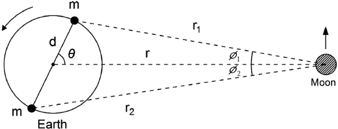

  

  The relative motions and positions of Earth and Moon

  Meanwhile, as we consider the Earth and Moon an isolated system immune to all external factors in this proposition, the overall angular momentum of this system should be the sum of the angular momentum of Earth’s $\left( {S_{E} } \right)$ and Moon’s rotation $\left( {S_{M} } \right)$ as well as the orbital angular momentum of both bodies $\left( {l_{E} \,{\text{and}}\,l_{M} } \right)$, which should be a non-changing value. Therefore, if Earth’s rotation slows down, the value of $l_{E} + l_{M}$ will have to go up. As for the angular momentum of Moon’s rotation $S_{M}$, we’ll later explain why it’s small enough to be disregarded.

  $$\begin{aligned} l_{E} + l_{M} & = M_{E} \left( {\frac{{M_{M} }}{{M_{E} + M_{M} }}r} \right)^{2} \omega + M_{m} \left( {\frac{{M_{E} }}{{M_{E} + M_{M} }}r} \right)^{2} \omega \\ & = \frac{{M_{M} M_{E} }}{{M_{E} + M_{M} }}r^{2} \omega \end{aligned}$$

  (4.76)

  Following Newton’s law of universal gravity, the gravity acting on Earth $\left( {\frac{{GM_{E} M_{M} }}{{r^{2} }}} \right)$ should be the product of $M_{E}$ and Earth’s acceleration, $\left( {\frac{{M_{M} }}{{M_{E} + M_{E} }}r} \right)\omega^{2}$, which is to say:

  $$\frac{{GM_{E} M_{M} }}{{r^{2} }} = M_{E} \left( {\frac{{M_{M} }}{{M_{E} + M_{M} }}r} \right)\omega^{2}$$

  (4.77)

  Equation (4.77) can be simplified as:

  $$\omega^{2} r^{3} = G\left( {M_{E} + M_{M} } \right)$$

  (4.78)

  Which we can then substitute into (4.76) and obtain:

  $$l_{E} + l_{M} = M_{M} M_{E} \left( {\frac{{G^{2} }}{{M_{E} + M_{M} }}} \right)^{1/3} \frac{1}{{\omega^{1/3} }}$$

  (4.79)

  According to (4.79), a smaller $\omega$ is the only possibility for $l_{E} + l_{M}$ to increase, and based on (4.77), a decreased $\omega$ means a longer distance between Earth and Moon (r), which scientists working on Project Apollo have confirmed at 3.8 cm per year with laser range-finding results showing the Moon’s gradual deviation from Earth. As $\omega$ is inversely proportional to the Moon’s rotation period, we can predict that it’ll take the body more than 27.3 days to complete a circle around Earth when its revolution is synchronized with the latter’s rotation.

• 2. Quantitative derivation based on revolving periods

  In this part, let’s first calculate the value of the overall angular momentum in the Earth-Moon system, which is $L = S_{E} + S_{M} + l_{E} + l_{M}$, and derive therefrom the period of Earth’s rotation and Moon’s revolution when both are synchronized. As defined previously, the angular momentum of Earth’s and Moon’s rotation is $S_{E} = I_{E} \varOmega$ and $S_{M} = I_{M} \omega$ respectively. After substituting the actual values, we will come to the following equations:

  $$\begin{aligned} S_{E} & = I_{E} \varOmega = 8.01 \times 10^{37} \left( {{\text{kg}}\;{\text{m}}^{2} } \right) \times \frac{2\pi }{{23.9 \times 3600\left( {\text{s}} \right)}} \\ & = 5.85 \times 10^{33} \left( {{\text{kg}}\;{\text{m}}^{2} /{\text{s}}} \right) \\ \end{aligned}$$

  (4.80)
  $$\begin{aligned} S_{M} & = I_{M} \omega = 8.77 \times 10^{34} \left( {{\text{kg}}\;{\text{m}}^{2} } \right) \times \frac{2\pi }{{27.3 \times 86,400\left( {\text{s}} \right)}} \\ & = 2.34 \times 10^{29} \left( {{\text{kg}}\;{\text{m}}^{2} /{\text{s}}} \right) \\ \end{aligned}$$

  (4.81)

  Again, if we substitute related values into (4.79), the combined orbital angular momentum of Earth’s and Moon’s revolution around the barycenter of the Earth-Moon system $\left( {l_{E} + l_{M} } \right)$ can be calculated to be:

  $$l_{E} + l_{M} = M_{M} M_{E} \left( {\frac{{G^{2} }}{{M_{E} + M_{M} }}} \right)^{1/3} \frac{1}{{\omega^{1/3} }} = 2.86 \times 10^{34} \left( {{\text{kg}}\;{\text{m}}^{2} /{\text{s}}} \right)$$

  (4.82)

  Judging from the three equations above, we can tell that the value of $S_{M}$ is smaller than $S_{E}$ and $l_{E} + l_{M}$ by $10^{4} \sim 10^{5}$ times. Therefore, we’ll simply disregard this parameter in the following steps, which leads us to:

  $$L = I_{E} \varOmega + M_{M} M_{E} \left( {\frac{{G^{2} }}{{M_{E} + M_{M} }}} \right)^{1/3} \frac{1}{{\omega^{1/3} }}$$

  (4.83)

  Then, we can add up the calculation results above to get the overall angular momentum in the Earth-Moon system:

  $$L = 3.44 \times 10^{34} \left( {{\text{kg}}\;{\text{m}}^{2} /{\text{s}}} \right)$$

  (4.84)

  When Earth’s rotation and Moon’s revolution are synchronized, $\varOmega$ and $\omega$ must be the same value, which we represent here as $\omega_{f}$. Due to the conservation of angular momentum, we can derive the below equation based on (4.84) and (4.85):

  $$I_{E} \omega_{f} + M_{M} M_{E} \left( {\frac{{G^{2} }}{{M_{E} + M_{M} }}} \right)^{1/3} \frac{1}{{\omega_{f}^{1/3} }} = 3.44 \times 10^{34} \left( {{\text{kg}}\;{\text{m}}^{2} /{\text{s}}} \right)$$

  (4.85)

  Substituting the actual values for the parameters in (4.85) will help us come to (4.86):

  $$8.01 \times 10^{37} \omega_{f} + 3.96 \times 10^{32} \omega_{f}^{ - 1/3} = 3.44 \times 10^{34}$$

  (4.86)

  Whose solution can be calculated as:

  $$\omega_{f} = 1.54 \times 10^{ - 6} \left( {{\text{rad}}/{\text{s}}} \right)$$

  (4.87)

  In other words, when Earth’s rotation and Moon’s revolution are synchronized, the shared period will become:

  $$T_{f} = \frac{2\pi }{{\omega_{f} }} = 4.08 \times 10^{6} \left( {\text{s}} \right)$$

  (4.88)

  If we apply the time of a current day, $T_{f}$ can be calculated at 47.2, meaning the Earth will need 47.2 days to complete a self-rotation.

• 3. Change of motion patterns in the Earth-Moon system over time

  When addressing this question, we need to first measure the influence of tidal waves with calculation before taking Fig. 4.15 into consideration. As previously mentioned, because the tidal bulges on both sides of the Earth are deemed equivalent masses (m), this value should be proportional to the tidal heights. Just as we’ve proved in Appendix 4.2, tidal heights are proportional to the cube of the distance between Earth and Moon (r); therefore, we know that $m \propto 1/r^{3}$. If we represent the distance between the point mass m and the center of Earth as d and assume that the angle $\theta$ formed by the line joining two tidal bulges and that between Earth and Moon wouldn’t change over time, we can calculate the torque generated by the Moon on Earth with the following steps:

  Fig. 4.15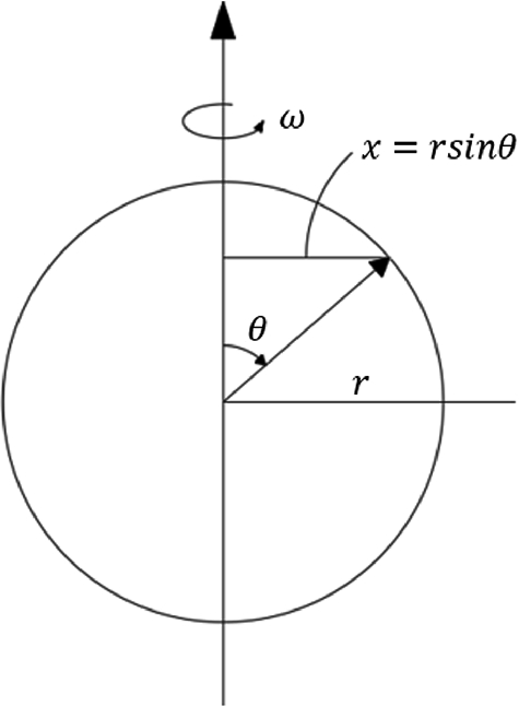

  

  The rotating coordinate system of Earth

  In Fig. 4.15, we can count on the law of cosines to calculate the drawing force exerted on the Moon by m, which is the point mass on Earth closest to it:

  $$F_{c} = \frac{{GmM_{M} }}{{r_{1}^{2} }} = \frac{{GmM_{M} }}{{r^{2} + d^{2} - 2rd\cos \theta }}$$

  (4.89)

  Similarly, the drawing force exerted on the Moon by the point mass on Earth furthest from it (represented as m as well) can also be calculated as:

  $$F_{f} = \frac{{GmM_{M} }}{{r_{2}^{2} }} = \frac{{GmM_{M} }}{{r^{2} + d^{2} + 2rd\cos \theta }}$$

  (4.90)

  Therefore, we know that the torque generated on the Moon by the point mass closest to it $\left( {\tau_{c} } \right)$ is:

  $$\tau_{c} = \left| {\vec{r} \times \overrightarrow {{F_{c} }} } \right| = rF_{c} { \sin }\left( {\pi - \phi_{1} } \right) = r\frac{{GmM_{M} }}{{r_{1}^{2} }}{ \sin }\phi_{1}$$

  (4.91)

  Again, with the law of cosines, (4.16) can be simplified as:

  $$\frac{d}{{{ \sin }\phi_{1} }} = \frac{{r_{1} }}{{{ \sin }\theta }} \Rightarrow { \sin }\phi_{1} = \frac{{d{ \sin }\theta }}{{r_{1} }}$$

  (4.92)

  Then, by substituting (4.92) into (4.91), we will come to the equation below:

  $$\tau_{c} = r\frac{{GmM_{M} }}{{r_{1}^{2} }} \cdot \frac{{d{ \sin }\theta }}{{r_{1} }} = \frac{{GmM_{M} rd\sin \theta }}{{\left( {r^{2} + d^{2} - 2rd\cos \theta } \right)^{3/2} }}$$

  (4.93)

  At this point, we can repeat the previous steps to calculate the torque generated on the Moon by the point mass furthest from it $\left( {\tau_{f} } \right)$ to be:

  $$\begin{aligned} \tau_{f} & = \left| {\vec{r} \times \overrightarrow {{F_{f} }} } \right| = rF_{f} \sin \left( {\pi - \phi_{2} } \right) = r\frac{{GmM_{M} }}{{r_{2}^{2} }}{ \sin }\phi_{2} \\ & = \frac{{GmM_{M} rd\sin \theta }}{{\left( {r^{2} + d^{2} + 2rd\cos \theta } \right)^{3/2} }} \\ \end{aligned}$$

  (4.94)

  Combining (4.93) and (4.94), we now know that the total torque generated by the two point masses on the Moon $(\uptau)$ is:

  $$\begin{aligned} {\tau } & = \tau _{c} - \tau _{f} \\ & = GmM_{M} rd\sin \theta \left[ {\frac{1}{{\left( {r^{2} + d^{2} - 2rd\cos \theta } \right)^{{3/2}} }} - \frac{1}{{\left( {r^{2} + d^{2} + 2rd\cos \theta } \right)^{{3/2}} }}} \right] \\ & = \frac{{GmM_{M} rd\sin \theta }}{{r^{3} }}\left[ {\left( {1 - \frac{{3d^{2} }}{{r^{2} }} + \frac{{3d\cos \theta }}{r}} \right) - \left( {1 - \frac{{3d^{2} }}{{r^{2} }} - \frac{{3d\cos \theta }}{r}} \right)} \right] \\ & = \frac{{GmM_{M} d\sin \theta }}{{r^{2} }} \cdot \frac{{6d\cos \theta }}{r} = \frac{{6GmM_{M} d^{2} \sin \theta \cos \theta }}{{r^{3} }} \\ \end{aligned}$$

  (4.95)

  Please note, that we should add a negative sign in (4.95) to signify the direction when considering the overall torque generated by the Moon on Earth’s tidal movements, as shown below:

  $$\tau = - \frac{{6GM_{M} md^{2} \sin \theta \cos \theta }}{{r^{3} }}$$

  (4.96)

  The negative sign in (4.96) means the direction of the torque is opposite from that of Earth’s rotation, which will hinder its movement and reduce its speed. Integrating $m \propto 1/r^{3}$ into (4.96), we can get the result $\tau = dS_{E} /dt \propto - 1/r^{6}$, which shows that the torque equals the change in angular momentum over time and has an inversely proportional relationship with r to the power of six, and because $L = S_{E} + S_{M} + l_{E} + l_{M}$ = a fixed value and $S_{M}$ is small enough to be disregarded, we can further derive:

  $$\frac{{d\left( {l_{E} + l_{M} } \right)}}{dt} \propto \frac{1}{{r^{6} }}$$

  (4.97)

  In addition, as (4.4) shows $l_{E} + l_{M}$ to be proportional to $1/\omega^{3}$, below equation can therefore be developed:

  $$\frac{{d\left( {\omega^{ - 1/3} } \right)}}{dt} = - \frac{1}{3}\omega^{{ - \frac{4}{3}}} \frac{d\omega }{dt} \propto \frac{1}{{r^{6} }}$$

  (4.98)

  And with (4.78), which tells us that $\omega^{2} r^{3}$ is a fixed value, we can derive $1/r^{6} \propto \omega^{4}$ therefrom and substitute it into (4.98):

  $$\omega^{{ - \frac{4}{3}}} \frac{d\omega }{dt} \propto - \omega^{4}$$

  (4.99)

  Which will lead us to:

  $$\frac{d\omega }{dt} \propto - \omega^{{\frac{16}{3}}}$$

  (4.100)

  If we insert C, a co-efficient of proportionality, into Eq. (4.100), it can be rewritten as:

  $$\frac{d\omega }{dt} = - C\omega^{{\frac{16}{3}}}$$

  (4.101)

  Then, by integrating the time in (4.101), from when $t = 0$ till $t = t_{f}$ (when Earth’s rotation is synchronized with Moon’s revolution), we can generate:

  $$t_{f} = \frac{3}{13C}\left[ {\omega_{f}^{ - 13/3} - \omega_{0}^{ - 13/3} } \right]$$

  (4.102)

  In which $\omega_{0}$ represents the current angular velocity of Moon’s revolution. As a result, we simply need to calculate the constant C at this point to obtain the time needed for the synchronization to happen.

  To get the value of C, we will make use of the 3.8 cm-result retrieved by researchers of Project Apollo, which is the annual increase in the distance between Earth and Moon. From (4.78), we know that:

  $$r = \left( {\frac{{G\left( {M_{E} + M_{M} } \right)}}{{\omega^{2} }}} \right)^{1/3}$$

  (4.103)

  If we differentiate (4.103) with respect to t, (4.104) will be derived therefrom:

  $$\frac{dr}{dt} = - \frac{2}{3}\left[ {G\left( {M_{E} + M_{M} } \right)} \right]^{{\frac{1}{3}}} \omega^{{ - \frac{5}{3}}} \frac{d\omega }{dt}$$

  (4.104)

  Then, from (4.104), we can calculate the current increase rate of the angular velocity:

  $$\left( {\frac{d\omega }{dt}} \right)_{t = 0} = - \frac{{3\omega_{0}^{5/3} }}{{2\left[ {G\left( {M_{E} + M_{M} } \right)} \right]^{1/3} }}\left( {\frac{dr}{dt}} \right)_{t = 0}$$

  (4.105)

  While a comparison of (4.105) and (4.101) leads us to (4.106):

  $$\frac{{3\omega_{0}^{5/3} }}{{2\left[ {G\left( {M_{E} + M_{M} } \right)} \right]^{1/3} }}\left( {\frac{dr}{dt}} \right)_{t = 0} = C\omega_{0}^{16/3}$$

  (4.106)

  The constant C can be written as:

  $$C = \frac{{3\omega_{0}^{ - 11/3} }}{{2\left[ {G\left( {M_{E} + M_{M} } \right)} \right]^{1/3} }}\left( {\frac{dr}{dt}} \right)_{t = 0}$$

  (4.107)

  At this point, we can substitute all the necessary parameters of physics into (4.107) and calculate C to be:

  $$\begin{aligned} C & = \frac{{3\left( {\frac{2\pi }{27.3 \times 86,400}} \right)^{ - 11/3} }}{{2\left[ {6.67 \times 10^{ - 11} \left( {5.97 \times 10^{24} + 7.35 \times 10^{22} } \right)} \right]^{1/3} }}\frac{0.038}{365.25 \times 86{,}400} \\ & = 6.73 \times 10^{6} \left( {s^{10/3} } \right) \\ \end{aligned}$$

  (4.108)

  Now, we can simply substitute the results from (4.108) and (4.87) into (4.102) to come to this final result:

  $$t_{f} = 4.78 \times 10^{17} \left( s \right) = 1.52 \times 10^{10} \left( {\text{years}} \right)$$

  (4.109)

  In other words, it’ll take 15.2 billion more years for Earth’s rotation and Moon’s revolution to be synchronized. However, this number is even larger than the universe’s age, and nobody knows for sure if the universe can continue to exist for that long. Simply put, it’s pretty much impossible for such co-orbiting to take place in the Earth-Moon system.

  Last but not least, we’d also like to prove the condition derived from the results by Project Apollo, i.e. when the Moon deviates 3.8 cm from the Earth every year, the latter’s rotation will gradually slow down, causing an average of a 1.7 ms-increase in one day on Earth every hundred years. Let’s start with Eq. (4.83), where L is a fixed value due to the conservation of angular momentum in the Earth-Moon system, which is why we can differentiate Eq. (4.83) over t and reach the following result:

  $$I_{E} \left( {\frac{d\varOmega }{dt}} \right)_{t = 0} = \frac{1}{3}M_{M} M_{E} \left( {\frac{{G^{2} }}{{M_{E} + M_{M} }}} \right)^{1/3} \frac{1}{{\omega_{0}^{4/3} }}\left( {\frac{d\omega }{dt}} \right)_{t = 0}$$

  (4.110)

  Then, (4.111) can be developed by substituting (4.105) into (4.110):

  $$\begin{aligned} \left( {\frac{d\varOmega }{dt}} \right)_{t = 0} & = - \frac{{\omega_{0}^{1/3} }}{{2I_{E} }}M_{M} M_{E} \left( {\frac{G}{{\left( {M_{E} + M_{M} } \right)^{2} }}} \right)^{1/3} \left( {\frac{dr}{dt}} \right)_{t = 0} \\ & = 5.59 \times 10^{ - 22} \left( {s^{ - 2} } \right) \end{aligned}$$

  (4.111)

  As the definition of the period is known to be $T = 2\pi /\varOmega$, we can differentiate T over t and substitute (4.111) to develop:

  $$\left( {\frac{dT}{dt}} \right)_{t = 0} = - \frac{2\pi }{{\varOmega^{2} }}\left( {\frac{d\varOmega }{dt}} \right)_{t = 0} = \frac{{2\pi \times 5.59 \times 10^{ - 22} }}{{\left( {\frac{2\pi }{86,400}} \right)^{2} }} = 6.64 \times 10^{ - 13}$$

  (4.112)

  As shown in (4.105), each day on Earth would be this much longer every hundred years:

  $$6.64 \times 10^{ - 13} \times 100 \times 365.25 \times 86,400 = 0.002\left( {\text{s}} \right)$$

  (4.113)

  Which equals 2 ms after conversion, extremely close to the previously mentioned 1.7 and 2.3 ms.

Appendix 4.5: How the Theory of Pendulum and Its Period Change When in Equatorial and Polar Regions

In 1673, Huygens proposed this theory in his book Horologium Oscillatorium: the ratio of a pendulum’s period to the time needed for an object to fall from the pendulum’s mid-point to its bottom equals the ratio between the perimeter and diameter of a circle whose radius is the length of the pendulum, and this ratio is 3.14159, exactly the $\pi$ we know today. In the form of an equation, this result of his can be written as $T = 2\pi \sqrt {l/g}$, where T and l represent the period and length of the pendulum respectively, while g is the acceleration of free fall objects (or gravitational acceleration, $9.81\;{\text{m}}/{\text{s}}^{2}$). Without the help of calculus or calculation tools, Huygens apparently had to count on his careful observation and precise measurements to obtain a formula with such accuracy³⁹. Luckily for us, though, we can simply resort to calculus to derive this pendulum equation:

$$T = 2\pi \sqrt {\frac{l}{g}}$$

(4.114)

Amplitude is generally supposed to be very small in the example calculations in common textbooks so that the pendulum movement can be seen as simple harmonic motion, a basis on which the angular frequency of very small vibrations can be easily calculated with Eq. (4.114). However, here we would like to give up this convenient condition by taking the range limit off the amplitude and first calculate the period of a pendulum with normal swing angles before applying the result to the case of minimum angles, whose result will prove the same as in common textbooks.

Now, let’s consider a pendulum whose bob has the mass m and the ceiling from which the pendulum hangs to be the zero point of potential energy. Under this circumstance, the sum of the pendulum’s momentum and potential energy when it travels furthest from the equilibrium position (swing angle $\theta = \theta_{0}$, ${\text{speed}} = 0$, potential energy = maximum) should equal that when the bob swings to whichever point on its trajectory $\left( {\theta < \theta_{0} } \right)$, which can lead us to this equation below:

$$\frac{1}{2}m\left( {l\dot{\theta }} \right)^{2} - mgl\cos \theta = 0 - mgl\cos \theta_{0}$$

(4.115)

Then, (4.115) can be slightly simplified to become:

$$\dot{\theta } = \sqrt {\frac{2g}{l}\left( {\cos \theta_{0} - \cos \theta } \right)}$$

(4.116)

In the following, firstly, we’re going to change the order of integration and calculate the integral value of (4.117). Please note that the range of integral is 0 to $\theta_{0}$, accounting for 1/4 of the period, so we will need to multiply the result by 4, which leads us to this equation below:

$$T = \int {dt} = 4\sqrt {\frac{l}{2g}} \int\limits_{0}^{{\theta_{0} }} {\frac{d\theta }{{\sqrt {\cos \theta - \cos \theta_{0} } }}}$$

(4.117)

Equation (4.117) represents the period for pendulums with normal swing angles, but as this equation contains an elliptic function and is therefore hard to integrate, we will need to assume the angle to be extremely small, a condition that can help us derive (4.118):

$$\cos \theta \approx 1 - \frac{{\theta^{2} }}{2}$$

(4.118)

On the other hand, if we simplify the elliptic function in (4.117), which we can then integrate, the process will yield the below equation, which represents the pendulum period:

$$T = \int dt = 4\sqrt {\frac{l}{g}} \mathop \int \limits_{0}^{{\theta_{0} }} \frac{d\theta }{{\sqrt {\theta_{0}^{2} - \theta^{2} } }} = 4\sqrt {\frac{l}{g}} \left( {\sin^{ - 1} \frac{\theta }{{\theta_{0} }}} \right)_{0}^{{\theta_{0} }} = 2\pi \sqrt {\frac{l}{g}}$$

(4.119)

As Earth’s is an oblate spheroid and rotates around its axis once every 24 h, the pendulum period is affected by Earth’s shape and rotation when placed at locations of different latitudes. As for the respective influences of both factors, we will conduct an analysis based on Eq. (4.119). Let’s start by considering how the period would change when the pendulum is placed in polar and equatorial areas. With the substitution of the average equatorial radius $\left( {R = 6738.14\;{\text{km}}} \right)$ and the polar radius $\left( {r = 6356.76{\text{km}}} \right)$, the difference can be calculated using (4.120),

$$\Delta T = 2\pi \sqrt l \left( {\frac{1}{{\sqrt {GM/R^{2} } }} - \frac{1}{{\sqrt {GM/r^{2} } }}} \right) \approx T\left( {\frac{R - r}{R}} \right)$$

(4.120)

Whose result would be:

$$\frac{\Delta T}{T} \approx 0.057$$

(4.121)

As a second step, let’s look at how the centrifugal force from Earth’s rotation affects the period when the pendulum is placed near the equator. Due to the effect of rotation, the gravitational field in the equatorial regions lacks the centrifugal acceleration $\Delta g = R\omega^{2} = 0.036\;{\text{m}}/{\text{s}}^{2}$ ($\omega$ representing the rotational angular velocity) compared to the fields that are not affected by Earth’s rotation. Therefore, the difference caused by the self-rotation of Earth in the pendulum period would be:

$$\Delta T = 2\pi \sqrt l \left( {\frac{1}{{\sqrt {g - \Delta g} }} - \frac{1}{\sqrt g }} \right) \approx T\left( {\frac{1}{2}\frac{\Delta g}{g}} \right)$$

(4.122)

Which can lead us to this result below:

$$\frac{\Delta T}{T} \approx 0.0018$$

(4.123)

A comparison of the two calculations above shows the fact that the difference caused by Earth’s rotation is almost 30 times smaller than that by varying radiuses in equatorial and polar regions.

Appendix 4.6: Calculating the Difference Between Earth’s Equatorial and Polar Radiuses

For details, please see Maxwell [22], pp. 494–496.

When calculating the degree of the increase in Earth’s equatorial radius (h) under the influence of self-rotation, we need first to suppose that (1) Earth’s mass is evenly distributed with the density of ρ, (2) it’s only affected by the gravitational force of its own and the centrifugal force from its self-rotation, while the influences of its revolution and the gravity of other astronomical bodies, such as the Sun, should all be disregarded, (3) it rotates at a fixed angular velocity of ω, with all possible movements of its axis disregarded, and (4) changes in the equatorial radius caused by its rotation are by far smaller than its varying radius, i.e. $h \ll r$. With all the conditions specified, let’s now try to calculate the value of h with the law of energy conservation.

In the rotating coordinate system illustrated in Fig. 4.15, the Earth has two types of potential energy, one from the universal gravitation, the other from the centrifugal force of its rotation. If Earth’s average radius is r (retrieved by calculating the average of radiuses at different locations over the solid angle of the entire Earth), the gravitational energy at any point on Earth can be represented approximately as mgh since $h \ll r$. Please note that h refers to the difference between r and the actual radius of each location on Earth’s surface.

As for the centrifugal potential energy, it can be obtained by integrating the centrifugal force $m\omega^{2} x$ over x, which represents the vertical distance between any point on Earth’s surface and its axis of rotation. Therefore, the centrifugal potential energy can be derived as:

$$- \int {m\omega^{2} xdx} = - \frac{1}{2}m\omega^{2} x^{2}$$

(4.124)

As we’ve assumed the mass of Earth is evenly distributed, the entire spherical surface should be an equipotential plane. Otherwise, the gradient of potential energy would cause a working force that leads to the redistribution of surface mass. As a result, the conservation of Earth’s overall potential energy can be written as:

$$mgh - \frac{1}{2}m\omega^{2} x^{2} = {\text{constant}}$$

(4.125)

If we substitute $x = r\sin \theta$, which reflects the shape of Earth’s surface, into (4.125), we can derive the change function $h\left( \theta \right)$, which shows how the degree of Earth’s deformation changes with latitude:

$$h\left( \theta \right) = \frac{{\omega^{2} r^{2} }}{2g}\sin^{2} \theta + C$$

(4.126)

We can then substitute $\theta = \pi /2$ and $\theta = 0$ into the function to calculate the change in equatorial $\left( {h\left( {\pi /2} \right)} \right)$ and polar $(h(0))$ radiuses, the difference between the two results being:

$${\text{h}}\left( {\frac{\pi }{2}} \right) - h\left( 0 \right) = \frac{{\omega^{2} r^{2} }}{2g} = \frac{{\left( {\frac{2\pi }{{86,400\;{\text{s}}}}} \right)^{2} \left( {6380\;{\text{km}}} \right)^{2} }}{{2 \times \frac{{9.8\;{\text{m}}}}{{s^{2} }}}} \approx 11\;{\text{km}}$$

(4.127)

One thing to be noted here is that the difference calculated from (4.127), which is supposed to reflect the difference between equatorial and polar radiuses, is approximately half of the actual value $(21.4\;{\text{km}})$ only. In other words, merely considering the influences of Earth’s two types of potential energy is apparently not thorough enough, which is why we need to further conduct an analysis to explore possibly important factors that have been excluded.

Therefore, let’s take a look at the previously derived Eq. (4.126) again and try to pinpoint the value of the integral constant C. To do this, we’ll first need to suppose the overall mass of Earth wouldn’t change due to its deformation, which is to say that the mass of the bulges near the equator would equal that of the hollows in polar areas, as shown in Fig. 4.16. Consequently, if we integrate $h\left( \theta \right)$, the change function of Earth’s deformation over the angles of the entire orb, the result should be zero:

Fig. 4.16

A schematic illustration of the shape-change of Earth’s surface due to rotation

$$\mathop \int \limits_{0}^{\pi } h\left( \theta \right) \cdot 2\pi \sin \theta d\theta = 0$$

(4.128)

We can then substitute (4.126) into (4.128), which we will subseqently integrate and retrieve the value of C as:

$$C = - \frac{{\omega^{2} r^{2} \sin^{2} \theta }}{3g}$$

(4.129)

Then, the substitution of C back into (4.126) and a bit of simplification will yield:

$$h\left( \theta \right) = \frac{{\omega^{2} r^{2} }}{6g}\left( {3\sin^{2} \theta - 2} \right)$$

(4.130)

In the derivation process above, we disregarded the tiny influence of Earth’s shape (an oblate spheroid, rather than a perfectly round sphere) on the gravitational energy on its surface. In other words, we simply need to take the masses deviating from the spherical frame back into consideration now. As the bulges and hollows are all quite thin (the red and blue sections are negative and positive masses respectively, as shown in Fig. 4.16), we can consider them concentrated on Earth’s surface, with the density of $\rho h\left( \theta \right)$.

For the purpose of calculation, we’ll still suppose $h\left( \theta \right)$ to be proportional to $3\sin^{2} \theta - 2$, but related parameters are slightly different:

$$h(\theta ) = f \times \frac{{\omega^{2} R^{2} }}{6g}(3\sin^{2} \theta - 2) = \beta (3\sin^{2} \theta - 2)$$

(4.131)

To obtain the value of f, let’s consider the potential energy at (R, 0, 0) and (0, 0, R), which represent a point on the equator and the North Pole respectively, to be the same, thereby deriving the below equation:

$$\begin{aligned} & \Rightarrow - 2mg\beta - \int_{0}^{2\pi } {\int_{0}^{\pi } {\frac{{Gm\rho \beta (3\sin^{2} \theta - 2)}}{{R\sqrt {2(1 - \cos \theta )} }}} } R^{2} \sin \theta d\theta d\phi + 0 \\ & = mg\beta - \int_{0}^{2\pi } {\int_{0}^{\pi } {\frac{{Gm\rho \beta (3\sin^{2} \theta - 2)}}{{R\sqrt {2(1 - \sin \theta \cos \phi )} }}} } R^{2} \sin \theta d\theta d\phi - \frac{{m\omega^{2} R^{2} }}{2} \\ \end{aligned}$$

(4.132)

As (4.132) is developed under the assumption that the mass of Earth is evenly distributed, the density $\rho$ can be replaced with $M/\frac{4}{3}\pi r^{3}$ along with the substitution of ${\text{g}} = {\text{GM}}/r^{2}$ and yield the following result after integration:

$$\begin{aligned} 1 & = f\left\{ {1 - \int_{0}^{{2\pi }} {\int_{0}^{\pi } {\left( {\frac{1}{{\sqrt {1 - \sin \theta \cos \phi } }} - \frac{1}{{\sqrt {1 - \cos \theta } }}} \right)\frac{{(3\sin ^{2} \theta - 2)\sin \theta d\theta d\phi }}{{4\sqrt 2 \pi }}} } } \right\} \\ & \approx f(1 - 0.6) \Rightarrow f \simeq 2.5 \\ \end{aligned}$$

(4.133)

As the value of integral in (4.133) is approximately 0.6, f can be calculated to be 2.5, which we can then substitute back into Eq. (4.131) and reach the result of the difference in Earth’s radiuses at $11\;{\text{km}} \times 2.5 = 27.5\;{\text{km}}$, this time larger than the actual value of $22\;{\text{km}}$. Such deviation is likely to be caused by our excluding the fact that Earth’s mass isn’t evenly distributed. If we take into consideration that the density near the Earth’s surface is lower than that of the interior, the integral of (4.133) should come smaller than 0.6, while f would be lower than 2.5 as well. This way, the final result would also be closer to the actual value.

Appendix 4.7: Feynman’s Geometrical Approach of Proving Planetary Orbits to Be Elliptic

In his purely geometrical approach to determining the shape of planetary orbits around Sun, Feynman supposed the Sun to be a fixed point due to its far larger mass than the Earth before seeking to prove the latter’s revolving orbit to be elliptic⁴⁰. Below are the three parts of his geometrical derivation.

• 1. Take the velocity vectors of Earth’s revolution at all moments and collect them together so their tails sit at a single point. This way, the tips would actually trace out a perfect circle, as shown in Fig. 4.17. Below is the proving process:

  Fig. 4.17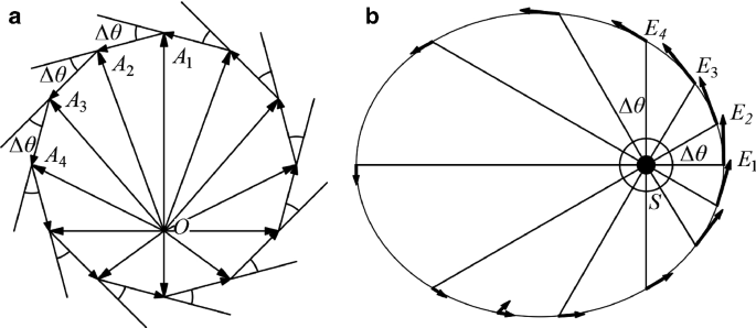

  

  The velocity vectors of Earth’s revolution at all moments. a A circle; b an ellipse

  Proof

  As shown in Fig. 4.17b, if we represent the Sun as S and divide the trajectory of Earth into equal parts with $E_{1} ,E_{2} ,E_{3} \ldots$ as the points of section, that means $\angle E_{1} SE_{2} = \angle E_{2} SE_{3} = \angle E_{3} SE_{4} = \cdots = \Delta \theta$. We can then draw the velocity vectors of Earth when it’s located at $E_{1} ,E_{2} ,E_{3} \ldots$ (i.e. $\overset{\lower0.5em\hbox{$\smash{\scriptscriptstyle\rightharpoonup}$}}{{OA_{1} }} ,\overset{\lower0.5em\hbox{$\smash{\scriptscriptstyle\rightharpoonup}$}}{{OA_{2} }} ,\overset{\lower0.5em\hbox{$\smash{\scriptscriptstyle\rightharpoonup}$}}{{OA_{3} }} \ldots$ in Fig. 4.17a). This way, $\overset{\lower0.5em\hbox{$\smash{\scriptscriptstyle\rightharpoonup}$}}{{A_{1} A_{2} }}$ can be seen as the change in Earth’s velocity when it travels from $E_{1}$ to $E_{2}$, $\overset{\lower0.5em\hbox{$\smash{\scriptscriptstyle\rightharpoonup}$}}{{A_{2} A_{3} }}$ that from $E_{2}$ to $E_{3} \ldots$ and so on. As a next step, we will need to find the limit of $\Delta \theta \left( {\Delta \theta \to 0} \right)$ so that the instantaneous acceleration over $\Delta t$ can be calculated by dividing $\overset{\lower0.5em\hbox{$\smash{\scriptscriptstyle\rightharpoonup}$}}{{A_{1} A_{2} }}$ by the time period.

At this point, however, we have to first prove the change in velocity over $\left| {\overset{\lower0.5em\hbox{$\smash{\scriptscriptstyle\rightharpoonup}$}}{{A_{k} A_{k + 1} }} } \right|$ to be a fixed number regardless of the value of k. If the distance between $E_{k}$ and the Sun is r, we can develop the following equation based on Newton’s law of universal gravitation:

$$\frac{{\left| {\overset{\lower0.5em\hbox{$\smash{\scriptscriptstyle\rightharpoonup}$}}{{A_{k} A_{k + 1} }} } \right|}}{\Delta t} = \frac{GM}{{r^{2} }}$$

(4.134)

It’s true that $\Delta t$ and r both change with k, but due to the conservation of angular momentum, we know that:

$$r^{2} \frac{\Delta \theta }{\Delta t} = {\text{non - changing value}}$$

(4.135)

Then, the substitution of (4.135) into (4.134) would yield:

$$\left| {\overset{\lower0.5em\hbox{$\smash{\scriptscriptstyle\rightharpoonup}$}}{{A_{k} A_{k + 1} }} } \right| \propto \Delta \theta$$

(4.136)

As the $\Delta \theta$ corresponding to each $\left| {\overset{\lower0.5em\hbox{$\smash{\scriptscriptstyle\rightharpoonup}$}}{{A_{k} A_{k + 1} }} } \right|$ is the same, we know that $\left| {\overset{\lower0.5em\hbox{$\smash{\scriptscriptstyle\rightharpoonup}$}}{{A_{k} A_{k + 1} }} } \right|$ is a fixed value. We’ve also noticed that when $\Delta \theta$ approaches the limit $(\Delta \theta \to 0)$, $\overset{\lower0.5em\hbox{$\smash{\scriptscriptstyle\rightharpoonup}$}}{{A_{k} A_{k + 1} }}$ and $\overset{\lower0.5em\hbox{$\smash{\scriptscriptstyle\rightharpoonup}$}}{{E_{k} O}}$ are in the same direction. In addition, the angle of $\Delta \theta$ between $\overset{\lower0.5em\hbox{$\smash{\scriptscriptstyle\rightharpoonup}$}}{{E_{k} O}}$ and $\overset{\lower0.5em\hbox{$\smash{\scriptscriptstyle\rightharpoonup}$}}{{E_{k + 1} O}}$ means $\overset{\lower0.5em\hbox{$\smash{\scriptscriptstyle\rightharpoonup}$}}{{A_{k} A_{k + 1} }}$ and $\overset{\lower0.5em\hbox{$\smash{\scriptscriptstyle\rightharpoonup}$}}{{A_{k + 1} A_{k + 2} }}$ form the same angle as well.

Summarizing the derivation above, we can confirm that:

• (1) $\left| {\overset{\lower0.5em\hbox{$\smash{\scriptscriptstyle\rightharpoonup}$}}{{A_{k} A_{k + 1} }} } \right|$ is a fixed value.

• (2) $\overset{\lower0.5em\hbox{$\smash{\scriptscriptstyle\rightharpoonup}$}}{{A_{k} A_{k + 1} }}$ and $\overset{\lower0.5em\hbox{$\smash{\scriptscriptstyle\rightharpoonup}$}}{{A_{k + 1} A_{k + 2} }}$ constantly form the angle $\Delta \theta$.

As such, we can confirm that all the $A_{k}$ will fall on the circumference of the circle whose center is C. Also, if the angle swept by Earth from $E_{i}$ to $E_{j}$ during its revolution around the Sun is $\theta$, $\angle {\text{A}}_{\text{i}} {\text{CA}}_{\text{j}}$ would also equal $\theta$.

• 2. If we, in the circle shown in Fig. 4.19, choose a point other than the center S and represent this eccentric point as D before choosing another point B on the circumference for the perpendicular bisector of $\overline{BD}$ to intersect with $\overline{BS}$ at E and rotate B for a full circle, the trajectory of E would be an ellipse. Below is the proving process:

Proof

As E falls on the perpendicular bisector of BD, we know that $\overline{ES} + \overline{ED} = \overline{ES} + \overline{EB} = \overline{BS}$, regardless of where B or E is. And by simply applying the definition of ellipse, we can prove that the trajectory of E is elliptic.

• 3. Below is the process of proving the Earth’s orbit to be elliptic by combining the results of Part 1 and 2.

Proof

If we rotate Fig. 4.18a by 90° clockwise, we’ll find it identical with Fig. 4.19, with O, C, $\overset{\lower0.5em\hbox{$\smash{\scriptscriptstyle\rightharpoonup}$}}{OA}$, and the radius $\overline{CA}$ overlapping with D, S, $\overset{\lower0.5em\hbox{$\smash{\scriptscriptstyle\rightharpoonup}$}}{DB}$, and $\overline{SB}$. In addition, the transition from Figs. 4.18a to 4.19 also rotates each velocity vector by 90° clockwise; in other words, as long as we rotate $\overset{\lower0.5em\hbox{$\smash{\scriptscriptstyle\rightharpoonup}$}}{DB}$ using the middle point of $\overline{DB}$ as a center by 90° counter-clockwise, the vector will return to its original direction, same as the tangential direction at point E on the elliptical trajectory in Fig. 4.19. Therefore, all we need to confirm is that this point would overlap with E in Fig. 4.18b. As we already know that the rotating angle of $\overline{ES}$ around S in Fig. 4.19 equals that of $\overline{CA}$ around A in Fig. 4.18a, and the results of Part 1 have also told us that the angle equals that of the rotation of $\overline{ES}$ around S in Fig. 4.18b, we can confirm that the ellipse in Fig. 4.18b and that in Fig. 4.19 actually has an equivalence relation, and that both can represent Earth’s revolving orbit. As such, it is proved that the ellipse in Fig. 4.19 is exactly the Earth’s revolving trajectory shown in Fig. 4.18b.

Fig. 4.18

A schematic illustration of the relationship between a the circular orbit and b the elliptic orbit

Fig. 4.19

A schematic illustration of the relative positions of the center S, the eccentric point D and a chosen point B