Modular Product Variety Generator Based on the Modified Genetic Algorithm: A Lego Plane

Abstract

Mass customization is a business strategy that aims at satisfying individual customer needs and provides them a large product mix. To achieve this goal, it is necessary to manage the product life cycle activities especially the volume and variety of products which have to be easily customizable. Designing modular products increases the possibility of obtaining customizable products. The modular design consists of breaking down a product into more or less independent sub-elements called modules. This paper focuses on setting up a Genetic-based automatic product variants generator. The product used as the testbed is a LEGO plane composed of bricks. Different operators are used for selection, crossover and mutation of genes. Each final plane assembly is qualified based on some criteria to respect pre-defined constraints. The obtained final assemblies are discussed at the end of the paper to highlights future challenges.

1 Introduction

Today, a product exists in several variants. The Renault Megane II, for example, is produced in a few thousand variants. Mass customization is a business strategy that aims at satisfying individual customer needs by providing a large product mix. Consumer demand for ever more differentiated products, generated the notion of a variety in early 80s. During the product design, it is therefore necessary to take into account of product variety and modularity. The modular design consists of breaking down a product into more or less independent sub-elements called modules that are bundled as a unit, and which serve identifiable functions. The differentiation of the finished product is obtained by defining modules and their interfaces.

In this context, this work focuses on the design of a computer tool for the generation of variants of a product composed of LEGO bricks using MATLAB language. These bricks of LEGO represent the modules to assemble. Of course, this research work does not take account more sophisticated concepts such as architecture determination, various types of exchanges between modules and so on; it remains focused on some aspects of a product definition. The following section will present the general idea about the concept of product variety as well as its advantages and disadvantages. The proposed methodology is introduced in Sect. 3 followed by presentation of the case study in Sect. 4. Section 5 focuses on the resolution technique which is the genetic algorithm, with some modifications. Finally, we discuss the obtained results before concluding by research perspectives.

2 Product Variety

Over the past decade, many research activities have been deployed to develop methods and tools to facilitate the design of product platforms and product families to provide cost-effective product variety and customization. The product platform is a relatively broad set of components, physically connected and forming a stable subset, common to different finished products [1]. Similarity in products configuration can led us to the notion of product family. A product family is a class, and variant products are instances of that family. Each instance is obtained by choosing different values of attributes [2]. According to [3] the term product family is defined as a group of interrelated products that are derivatives of a platform produced to satisfy a variety in the marketplace. The variety of products is a fundamental element of the commercial offer. However, it is subject to positive and negative pressures. Business objectives, such as the fight against competition and the arrival of new technologies, are pushing for an increase in variety to best meet customer needs. On the other hand, a variety that is too high becomes a brake on economic growth, particularly due to, for example, too much confusion that it can induce. Nevertheless, above all are the concerns of production in favor of the variety mastery. A too high variety generates too many references items to procure, store, manage, etc. Negative pressures therefore come mainly from manufacturing concerns.

Industrialists are therefore seeking to find a solution to this. In the literature [4], the modularity of products is considered among the best solutions. From a commercial point of view, a modular product presents several varieties by combining the different possible configurations of the modules. In addition, modularity reduces the complexity of the operations of the production process.

A huge number of modular methods have been proposed in the literature such as the graph and matrix partitioning method by [5], the mathematical programming method [6], the clustering methods, Genetic Algorithm [7] or Artificial Intelligence.

Generally, in previous researches, there are two main steps: (1) regroup components or identify all the modules of the product and (2) produce different product variants by testing different configurations. In addition, a technique such as UML diagrams, DSMs, IDEF0 and OPM is used to model the product architecture. But, we think that each different architecture representation is best suited for a specific purpose and not fit exactly to our need and requirements in some cases.

That’s why in this paper we propose a new modular methodology for product variety generation with definition of a modular architecture representation. This study aims to contribute to this growing area of research by exploring the modularity in LEGO modelling which we consider as another way of seeing the product from a modular point of view. To our knowledge, the use and building of products in LEGO is conventionally done with the aim of designing prototypes for products and models, and this paper is the first attempt to generate alternatives or varieties of product using different design constraints. Problem resolution is done by modified GA.

3 Product Architecture and Variety: General Methodology

As said previously, we need first to define and model the Product architecture. Inspired by the definition given by [8] as “The structure (in terms of components, connections, and constraints) of a product”, we propose in Fig. 1 our approach. A Product is a set of physical (components), logical (constraints) and functions connected together. In other words, Product architecture is considered as the scheme by which the functions of the product are arranged into physical chunks controlled via the existence of constraints and interacted via connections.

Fig. 1.

Product architecture representation (Color figure online)

Four types of connections are identified here (represented in different colors in Fig. 1). One or more physical component(s) can be regrouped with single or multiple function(s) in one block called ‘Module’. The Module includes also the different connections that link these functions and physical components together (type (a), (b) or (c)). And two modules are connected together if there are connections type (a), (b) or (c) between two elements (function or physical component) where each element belong to one of these modules. The steps of our methodology for variety generation are:

• 1. Identify the different modules, their physical and functional composition, interaction between them and connection with the constraints

• 2. Model modules as LEGO bricks and translate the different constraints and connections into equations

• 3. Simulate different combinations and find new product variants.

4 LEGO Plane

We consider that a product $P$ that can be modelled into LEGO bricks, is the result of the assembly of a set of blocks, called “modules” $M_{i}$ on a platform (a set of LEGO bricks that are fixed in specific position).

$$ P\; = \;Platform\; + \;\mathop \sum \nolimits_{i} M_{i} $$

(1)

Our case of study is a LEGO plane, modelled in Fig. 2 composed by a platform and $18$ modules. We denote $n_{m}$ the number of modules in one solution. The goal is to generate new plane variants respecting defined criteria.

Fig. 2.

3D LEGO plane model

Each module can contain one or more LEGO bricks and it is characterized by a function and a geometric structure. For example, an “engine” module contains two bricks has a rectangular structure of defined dimensions and performs the energy transformation. We consider a discrete space of three dimensions $\left( {x, y, z} \right)$; with $x_{max} \,\,, y_{max} \,\,, z_{max}$ standing for the maximum dimensions of the space along the axis; $O\left( {1,1,1} \right)$ is the point of origin. A product can therefore be represented within the solution space $(x_{max} \times y_{max} \times z_{max} )$. Each module $M_{i}$ of dimension $\left( {n_{i} \times m_{i} \times p_{i} } \right)$ is represented by a matrix $Mat_{i}$ of having the same dimension and containing the value $i$ in all the cells.

$$ Mat_{i} \left( {x,y,z} \right) = i \forall x \in \left[\kern-0.15em\left[ {1,n_{i} } \right]\kern-0.15em\right], \forall y \in \left[\kern-0.15em\left[ {1,m_{i} } \right]\kern-0.15em\right], \forall z \in \left[\kern-0.15em\left[ {1,p_{i} } \right]\kern-0.15em\right] $$

(2)

A module $M_{i}$ is characterized by:

• Geometric dimensions: $\left( {n_{i} \times m_{i} \times p_{i} } \right)$ length, width and height.

• A position vector $P\left( i \right) = \left[ {x_{i} , y_{i} , z_{i} } \right]$ that represents its position in the solution $S$, where $x_{i} ,y_{i}$ and $z_{i}$ represent coordinates of the Module $M_{i}$ in the solution space along the 3 dimensions.

• An orientation $O\left( i \right)$ signifying its orientation (‘H’ for horizontal or ‘V’ for vertical) in the solution S.

So, inserting the same module, we can get two different solutions depending on the orientation value.

Given a Module where $\left\{\kern-0.15em\begin{array}{c} {Mat_{i} ( {x,y,z}) {\,=\,} i \forall x \in [\kern-0.15em[ {1,n_{i} } ]\kern-0.15em], \forall y {\in\,} [\kern-0.15em[ {1,m_{i} } ]\kern-0.15em], \forall z {\in\,} [\kern-0.15em[ {1,p_{i} } ]\kern-0.15em]} \\ {P( i) = [ {x_{i} , y_{i} , z_{i} } ]} \\ \end{array}\right.$

If $O\left( i \right) =$ ‘H’ then

$$ S\left( {x + x_{i} - 1, y + y_{i} - 1, z + z_{i} - 1} \right) = i \forall x \in \left[\kern-0.15em\left[ {1,n_{i} } \right]\kern-0.15em\right], \forall y \in \left[\kern-0.15em\left[ {1,m_{i} } \right]\kern-0.15em\right], \forall z \in \left[\kern-0.15em\left[ {1,p_{i} } \right]\kern-0.15em\right] $$

(3)

Suppose now a solution where $O\left( i \right) =$ ‘V’, we get:

$$ S\left( {x + x_{i} - 1,\,y + y_{i} - 1,\,z + z_{i} - 1} \right) = i \forall x \in \left[\kern-0.15em\left[ {1,m_{i} } \right]\kern-0.15em\right],\,\forall y \in \left[\kern-0.15em\left[ {1,n_{i} } \right]\kern-0.15em\right],\,\forall z \in \left[\kern-0.15em\left[ {1,p_{i} } \right]\kern-0.15em\right] $$

(4)

Now, if we generalize for all the solution matrix values:

$$ \begin{array}{*{20}c} {S\left( {a,b,c} \right) = \left\{ {i,\,if\,\exists i,\,where\left\{ {\begin{array}{*{20}c} {Mat_{i} \left( {a - x_{i} + 1,\,b - y_{i} + 1,\,c - z_{i} + 1} \right) = i \forall \left\{ {\begin{array}{*{20}c} {\left\{ {\begin{array}{*{20}l} {a \in \left[\kern-0.15em\left[ {{\text{x}}_{\text{i}} ,{\text{x}}_{\text{i}} + n_{i} - 1} \right]\kern-0.15em\right]} \hfill \\ {b \in \left[\kern-0.15em\left[ {{\text{y}}_{\text{i}} ,{\text{y}}_{\text{i}} + m_{i} - 1} \right]\kern-0.15em\right]} \hfill \\ {c \in \left[\kern-0.15em\left[ {{\text{z}}_{\text{i}} ,{\text{z}}_{\text{i}} + p_{i} - 1} \right]\kern-0.15em\right]} \hfill \\ \end{array} } \right\}} \\ \cup \\ {\left\{ {\begin{array}{*{20}l} {a \in \left[\kern-0.15em\left[ {{\text{y}}_{\text{i}} ,{\text{y}}_{\text{i}} + m_{i} - 1} \right]\kern-0.15em\right]} \hfill \\ {b \in \left[\kern-0.15em\left[ {{\text{x}}_{\text{i}} ,{\text{x}}_{\text{i}} + n_{i} - 1} \right]\kern-0.15em\right]} \hfill \\ {c \in \left[\kern-0.15em\left[ {{\text{z}}_{\text{i}} ,{\text{z}}_{\text{i}} + p_{i} - 1} \right]\kern-0.15em\right]} \hfill \\ \end{array} } \right\}} \\ \end{array} } \right\}} \\ {P\left( i \right) = \left[ {x_{i} , y_{i} , z_{i} } \right]\quad \quad \quad \quad } \\ \end{array} } \right.} \right\}} \\ {0\,\,{\text{otherwise}}} \\ \end{array} $$

(5)

The platform represents the modules that are fixed (their position vector and orientation have a unique value that cannot be changed) and that exist in the chromosome. A solution is defined as a combination of placement of these matrices $Mat_{i}$ in solution space fitting constraints. Design rules and assembly constraints must be defined to ensure compliance of generated products with expected functions and specifications. Mathematical modelling of different Lego pieces, constraints and rules can be done using Matrices. These constraints are classified under 3 categories:

• Constraints on the modules (type (d)): for each module, attributes are defined

  • rotational constraint ($M_{i}$ can be rotated horizontally, vertically or both) $(H$, $V$, $H/V$)

  • assembly constraint above (assemble another module above $M_{i}$) ($YES, NO$)

  • assembly constraint below (assemble another module below $M_{i}$) ($YES, NO$)

  • assembly constraint on the right (assemble another module on the right side of $M_{i}$) ($YES, NO$)

• Constraints between the modules (type (a) or (b)), such as:

  • Plane wings must be in the front of the plane and distance between wings $M_{2}$ and the nose $M_{4}$ must be less than 50% of $M_{1}$ the platform length,

  • distance between $M_{1}$ and $M_{4}$ is null,

  • each module $M_{i} , \forall i \ne 4$ must have at least one module $M_{j} j \ne i$ assembled below or above,

  • the red light $M_{5}$ must be at the left side of the wing $M_{2}$ and the green one $M_{4}$ must be at right, etc…

• Constraints on the solution: The solution is a ($n_{s} \times m_{s} \times p_{s}$) matrix

  • $n_{s} \le x_{max} , m_{s} \le y_{max}$ and $p_{s} \le z_{max}$

  • All modules exist in the matrix and there is no overlap between modules

  • Each module exists ones a time

All these constraints are necessary to define a plane, but not sufficient to get a good plane. The goal is to design a computer tool using MATLAB and relying on the notion of the GA to generate from these Lego pieces all possible plane variants.

5 Genetic Algorithm Principle

Genetic Algorithm (GA) is an evolutionary algorithm inspired by Darwin’s theory of species evolution developed by [9]. It has proved its effectiveness in solving a wide variety of problems in various fields: robotics [10], facility layout problem, planning problem [11] and others [12,13,14]. For this reason, the GA is adopted in this paper.

The Genetic Algorithm starts with an initial population consisting of a set of individuals. Each individual is represented by a chromosome. This population evolves during a succession of iterations, called generations. At each iteration, three types of operators (selection, crossover and mutation) are applied to individuals in order to obtain new individuals. Several different operators can be used. This process of evolution is repeated until the satisfaction of a stopping criterion. The flow chart of different GA steps is shown in Fig. 3. In our case, we will focus particularly on the generation of a variety of LEGO products (an assembly of LEGO bricks).

Fig. 3.

Genetic Algorithm principle

• Step 1: chromosome encoding: Each individual is represented by a vector with $\left( {n \times m \times p} \right)$ columns as illustrated in Fig. 4. With $n$, $m$ and $p$ represent respectively the dimensions of a matrix $S$: number of rows, number of columns and number of layers. This matrix $S$ represents the matrix model of the product in a $3D$ space. Each cell of the matrix $S$ can have either the value $0$ (if there are no Lego bricks in the position $\left( {i, j, k} \right)$) or the value $x$ where $x$ is the index of the module $M_{x}$ which exists in the position $\left( {i,j,k} \right)$.

  Fig. 4.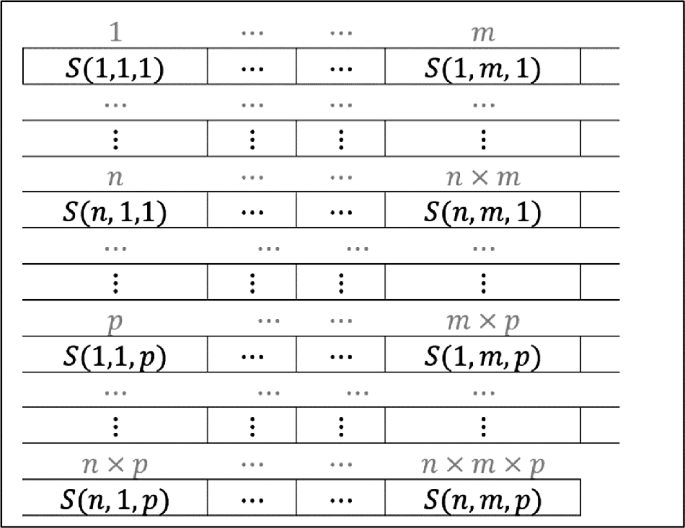

  

  Encoding of chromosome

• Step 2: Selection: The selection consists in choosing the individuals who will participate in the reproduction of the future generation. The selection operator adopted in this work is the random selection. It consists of choosing an individual in a random manner according to a uniform distribution.

• Step 3: Crossover: The crossover operator is used to combine the different parts of each parent. This operator plays a key role for the diversity of the population. It is applied with a certain probability named crossover probability. The crossing operator adopted here is specific to our case study. It has not been used before in other research works. As illustrated in Fig. 5, it is necessary to randomly choose two different cut-off points $x_{1}$ and $x_{2}$. The first child $C_{1}$ is created by keeping the first part of the first parent $P_{1}$ and the second part of $P_{2}$. The block between $x_{1}$ and $x_{2}$ consists of the random arrangement of the missing modules. The second child $C_{2}$ is made in the opposite way. NB: If a module is divided into two part: for example a part of module is before $x_{1}$ and the other is after $x_{1}$, as a result, the module belongs to the first part of the first child. As shown in Fig. 5, the cutoff point $x_{1}$ divides the module $M_{1}$ (yellow color) into two parts. So this module belongs to the first part of $E_{1}$.

  Fig. 5.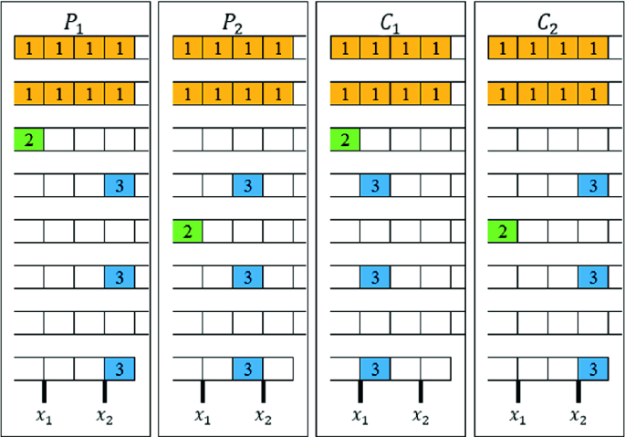

  

  Crossover operator (Color figure online)

• Step 4: Mutation: The mutation operator is used to apply some transformations on the chromosome structure with a low probability noted $p_{m}$. Its main objective is to keep the diversity of solutions. The mutation operator applied in this study is the “exchange operator”. The principle is to choose any random module to change its position as well as all the modules that are above it in the $3D$ matrix $S$. The new position of these modules will be randomly chosen from one of the vacant boxes following a random order.

• Step 5: Evaluation: The evaluation of solutions is done by assigning an X-weighting that measures the performance of each individual by taking into account criteria. Here we chose the feasibility (A), symmetry (B) and the stability (C). The score is computed as below:

  $$ SCORE = A \times \left( {1 + B} \right) - Coefficient \times C $$

  (6)
  $$ \begin{array}{*{20}l} { {\text{Where}}\quad \quad \quad \quad A = \left\{ {\begin{array}{*{20}c} {1 \,{\text{if}}\,{\text{the}}\, {\text{solution}}\, {\text{represents}}\, {\text{a}}\,{\text{plane }}} \\ {0\,\,{\text{otherwise}}} \\ \end{array} } \right\}} \hfill \\ {{\text{And}}\quad \quad \quad \quad \quad B = \left\{ {\begin{array}{*{20}c} {2 \,{\text{if}}\,{\text{the}}\,{\text{plane}}\, {\text{is}}\, {\text{symmetrical}}} \\ {1\,\,{\text{otherwise}}} \\ \end{array} } \right\}} \hfill \\ \end{array} $$
  $$ C = \left\{ {\begin{array}{*{20}c} {0\,{\text{if}}\,{\text{the}}\,{\text{plane}}\, {\text{is}} \,{\text{stable}} } \\ { {>}0\,\,{\text{otherwise}} } \\ \end{array} } \right\}\quad \quad {\text{and}}\quad \quad \quad \quad Coefficient = {1 \mathord{\left/ {\vphantom {1 {1000}}} \right. \kern-0pt} {1000}} $$

  A solution is considered as a plane if it responds to all constraints. Symmetry is defined here by the horizontal plane that cuts the matrix $S$ in half and passes through the point of gravity of the plane. Stability is computed by the difference of plane weight at right and left of the vertical plane that cuts the matrix $S$ in half and passes through the point of gravity of the plane.

• Step 6: Stopping criterion: The genetic algorithm evolves in several generations until the satisfaction of a stopping criterion. The criterion chosen in our case is a maximum number of iterations fixed at $100000$ iterations.

6 Results and Discussion

After execution of $100000$ iterations (in Table 1, the specification of our study), the developed algorithm have generated $22$ different variants of LEGO plane. They obey to all the constraints defined before. Some of them is symmetric, and others are stable planes (Different results are shown in Fig. 6 and represented as stars). Plane B represents the initial design which is symmetric and not stable with a score equal to $1.9933$. Plane A has the best score ($score = 2$) and represents the best variant that fit to the requirements of symmetry and stability. Some results (such as $Plane C$) are symmetric but not stable and others are stable but not symmetric (example $Plane D$ with a $score = 1$). The rest of solutions are planes also, and they are neither symmetric neither stable (the case of Plane E with a $score = 0.9933$). What is surprising is that the six Planes that we have provided to the algorithm as an input and considered as the initial population, are not the best alternatives in terms of score.

Table 1. Study specifications

Fig. 6.

Evaluation of different solutions

7 Conclusion

Product variety continues to be a major goal for companies, and architecting modular or platform-based product is becoming crucial in helping designers accomplish this. The aim of the present research was to generate new variants for a modular product. A LEGO model was used to express the modularity of the Plane. Based on a modified Genetic Algorithm (with new operators), a MATLAB program has been implemented to generate these new product variants. Results show that even if we use a small number of modules, the Genetic Algorithm is able to find in a short time (less than half an hour) product new alternatives. In this work we have chosen only three criteria to evaluate the product performances; further research might explore more criteria linked together in another combination. Some hypothesis may be considered as restrictive and need to be generalized in order to increase the degree of complexity, such as the possibility to generate solutions that contain more than 18 modules and where modules are used more than one time. In future work, the authors aim to compare different resolution techniques, such as particle swarm optimization “PSO” rather than Genetic Algorithm.