
Abstract
An important type of Newtonian deformable bodies are the ones in which the stress is a homogeneous function of the rate of strain. That is, when the stress and the rate of strain vanish simultaneously. The simplest such bodies are the ones for which the stress is a linear homogeneous function of the strain, that is the following relation holds:
where \(Y_{\mu \nu }^{\lambda \rho }\) is a tensor (the coupling tensor).The dimensions of \(Y_{\mu \nu }^{\lambda \rho }\) are [T]. These Newtonian deformable bodies we call elastic Newtonian bodies.
Access this chapter
Tax calculation will be finalised at checkout
Purchases are for personal use only
Notes
- 1.
This means that this tensor is an irreducible representation of the group SO(3).
- 2.
This result holds for any symmetric second order isotropic tensors, not only for the strain and the stress tensor.
- 3.
Here we have two positive definite metrics which are diagonalized simultaneously, that is, their principal axes coincide. See footnote 5 Chap. 2.
- 4.
The non-vanishing component is the \(\frac {\delta x}{y},\) that is, the xy and yx component only.
- 5.
We use the same E, σ because the continuum is isotropic, therefore the scalars on the surface of a sphere centered at the origin (here the origin of the principal directions of strain/stress) must have the same value.
- 6.
This is an invariant because the quantities E, σ being tensors are invariants.
- 7.
One can prove the invariance directly using the transformation rule (21.20). Indeed we have:
$$\displaystyle \begin{aligned} \sum_{\mu }\overset{\_}{t}_{\mu \mu }=\sum_{\mu }a_{\mu }^{\rho }a_{\mu }^{\lambda }t_{\rho \lambda }=\sum_{\mu }\delta ^{\rho \lambda }t_{\rho \lambda }=\sum_{\mu }t_{\rho \rho }\end{aligned} $$(21.21) - 8.
As we have already remarked the isotropy implies only that the tensors are symmetric, not diagonal!
- 9.
This is a key assumption!
- 10.
The (infinitesimal) surface dσ can be associated with a vector n normal to the surface whose length equals dσ. This is the vector dσ ν.
- 11.
In general the density of force in the direction specified by the vector A μ is given by t μν A ν.
- 12.
The material is assumed to be locally homogeneous and isotropic therefore E, σ are constants during the strain motion.
- 13.
The rhs is mass density times acceleration and the lhs is density of force. We apply Newton’s Second Law in the form: Total force density = mass density times acceleration. Acceleration is the second order time derivative of the strain vector.
- 14.
We give a second proof in terms of tensors. We have:
$$\displaystyle \begin{aligned} f^{\mu}=\varepsilon^{\mu\nu\rho}A_{\nu,\rho}+\phi^{,\mu} \end{aligned}$$and we assume that the vector
$$\displaystyle \begin{aligned} A_{\nu}=\varepsilon_{\nu\sigma\kappa}w^{\sigma,\kappa} \end{aligned}$$so that \(A_{,\nu }^{\nu }=0\) and
$$\displaystyle \begin{aligned} \phi=-w_{,\sigma}^{\sigma} \end{aligned}$$hence ε νσκ ϕ σ, κ = 0. The vector field w μ is an auxiliary vector field. Then we have:
$$\displaystyle \begin{aligned} f^{\mu}&=\varepsilon^{\mu\nu\rho}\varepsilon_{\nu\rho\sigma}w^{\sigma,\kappa }-(w_{,\sigma}^{\sigma})^{,\mu}=-\left( \delta_{\sigma}^{\mu}\delta_{\kappa }^{\rho}-\delta_{\sigma}^{\rho}\delta_{\kappa}^{\mu}\right) w^{\sigma,\kappa }-(w_{,\sigma}^{\sigma})^{,\mu}\\ &=-w_{\ldots..\kappa}^{\mu,\kappa}+(w_{,\rho}^{ \rho})^{,\mu}-(w_{,\sigma}^{\sigma})^{,\mu}=-w_{\ldots..\kappa}^{\mu,\kappa}. \end{aligned} $$The above remain true if we consider a constant in front of the definition of A ν, ϕ.
- 15.
Non-dissipative means that the wave preserves its form as it propagates. By this we mean that if at time t = 0 its form at the origin is f(r) where r is the position vector of a point in space – this is a snapshot or form of the wave – then at a time t the wave (snapshot) at the point r is f(r −V t) where V is the velocity of the wave.
- 16.
To be precise a vector f is uniquely determined if its divergence and curl are known throughout all of space, provided that f tends to zero like \(\frac {1}{r^{2}}\) as r →∞. See for example Vector and tensor Analysis by H. Lass McGraw-Hill 1950.
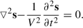
- 17.
We compute the velocity from the propagation equation of a non dissipative free wave, that is:

Author information
Authors and Affiliations
Rights and permissions
Copyright information
© 2019 Springer Nature Switzerland AG
About this chapter

Cite this chapter
Tsamparlis, M. (2019). The Stress: Strain Relation for Elastic Newtonian Deformable Bodies. In: Special Relativity. Undergraduate Lecture Notes in Physics. Springer, Cham. https://doi.org/10.1007/978-3-030-27347-7_21
Download citation
DOI: https://doi.org/10.1007/978-3-030-27347-7_21
Published:
Publisher Name: Springer, Cham
Print ISBN: 978-3-030-27346-0
Online ISBN: 978-3-030-27347-7
eBook Packages: Physics and AstronomyPhysics and Astronomy (R0)