Geometrically Intuitive Rendering of High-Dimensional Data

Abstract

Visualization is arguably the most powerful manual analytic method. However, as enterprise data have grown in size and complexity, supporting fast and intuitive data visualization has been become increasingly difficult. In particular, when the data being analyzed have many dimensions (e.g., feature vectors having many attributes), conventional methods, when they can be used at all, often make representational compromises that produce non-intuitive and misleading graphical products.

Three conventional methods for displaying sets of high-dimensional vectors on a flat computer display are described: pair-plots, feature-winnowing, and parallel coordinate plots. These are compared with two methods the authors have formulated, Recursive Stereographic Projection (RSP), and Tensor Projection (TP), for producing visual displays of high-dimensional discrete data that are fast, intuitive, navigable, and informative, and tend to preserve geometric characteristics of the original high-dimensional data such as, occlusion, proximity, intersection, relative scale, spatial extent, shape, and coherence.

Several real-world examples of intuitive 2-dimensional renderings of high-dimensional data are given. Suggestions for future research are made, and references provided.

1 Feature Vectors and Feature Spaces

Vectors and vector-valued functions will be indicated by underscoring, e.g., V, A(x); the norm of a vector is denoted |V|. The set of real numbers is denoted by R, and N-dimensional Euclidean space by RN.

A feature is a numeric value chosen to encode an attribute of an entity being modeled (e.g., size, quality, age, color, etc.). While features can be numbers, symbols, or complex data objects, they are usually coded in numeric form before modeling is performed.

Once features have been designated, a feature space can be defined for a domain by placing the features of each entity into an ordered array in a systematic way.

Each instance of an entity having the given features is then represented by a single point in n-dimensional Euclidean space, called its feature vector. The space in which the feature vectors reside is the feature space.

1.1 The Particular Benefits of Visualization

Visual analysis has significant advantages over tabular and chart-based analysis:

• 1. Visualization allows the analyst to develop “intuition” about the intelligence domain, detection of known and emerging patterns, and characterization of entity behaviors. When an analyst is able to see data, she develops an intuitive understanding of it that can be obtained in no other way.

• 2. Visualization can lead to the direct discovery of domain “rules”.

• 3. Visualization is an effective way to scan large amounts of data for “significant differences” between classes. If the icons representing interesting behaviors are well separated from uninteresting behaviors along some axis, this will be visually apparent. The feature that axis represents, then, accounts for some of the difference between interesting and uninteresting behaviors.

• 4. Visualization is a good technique for detecting poorly conditioned data. When data are plotted, errors in data preparation often show up as unexpected irregularities in the visual pattern of the data.

• 5. Visualization is a good technique for selecting a data model. For example, data that is normally distributed will have a characteristic shape. Visual analysis lets the analyst “see” which of several models might be most reasonable for a population being studied.

• 6. Visualization is a good technique for spotting outliers and missing data. When data are visualized, outliers (data not conforming to the general pattern of the population) are often easy to pick out. Missing records may show up as “holes” in a pattern, and missing fields within a record often break patterns in easily detectable ways.

1.2 Visualization Methods

The most effective pattern recognition equipment known to man is “wetware”: the mass of neurons between the users’ ears. Manual knowledge discovery is facilitated when data are presented in a form that allows the human mind to interact with them at an intuitive level. Visual data presentation provides a high-bandwidth, naturally intuitive gate to the human mind.

Data visualization is more than depiction of data in interesting plots. The goal of visualization is to help the analyst gain intuition about the data being observed. Therefore, visualization applications frequently assist the user in selecting display formats, viewer perspectives, and data representation schemas that foster deep intuitive understanding. Of particular importance is the fact that visualization allows fast mental correlation of many attributes at once: it makes the joint distribution of features accessible.

Several conventional techniques exist for the visualization of 2 and 3-dimensional data: scatter-plots of features by pairs, histograms, relationship trees, bar charts, pie charts, tables, etc. Modern visualization tools often include other capabilities (e.g., searching, sorting, scaling). Advanced functions might include:

• drill-down

• hyper-links to related data sources

• multiple simultaneous data views

• roam/pan/zoom

• select/count/analyze objects in display

• dynamic/active views (e.g., Java applets)

• using animation to depict a sequence or process

• creative use of color

• statistical summarization

• use of glyphs (icons indicating additional information about displayed objects)

When data have more than 3-dimensions, however, they become more difficult to conceptualize. Graphical techniques for representing high-dimensional data are often challenging to implement and use.

2 Classical Methods

• Many conventional methods have been developed for the representation of high-dimensional data. Most rely on some non-geometric way to retain some of the information lost when dimensions are suppressed:

• Using “glyphs”: indicating two features as spatial x-y coordinates, and other features using aliases such as color, shape, size, etc. This simple type of display is often supported by conventional OLAP tools.

• Performing orthographic projection (“feature winnowing”): using spatial dimensions to plot two or three features, while ignoring the rest

• Using trees and graphs to encode dimensions in different regions of the display (e.g., quadtrees)

• Plotting data in parallel coordinates, so that dimensions are spread horizontally across the display

2.1 Pair Plots

Pair plots are an extreme instance of feature-winnowing: plot the data in just two of the available N features and ignore the rest. As such, pair plots are not actually a method for visualizing high-dimensional data; but they are the most common approach to the dimensionality problem in practice.

When this approach is taken, there are two common strategies to mitigate information loss. Strategy 1 is to select the two features that are the most informative when used together. Strategy 2 is to plot thumbnails of every one of the N-choose-2 possible pairs of features.

These strategies have their own inherent problems. For Strategy 1, users will often choose to plot the data using the two features most highly correlated with the data being sought. However, since the most informative features are often correlated with each other, this strategy amounts to plotting data using redundant features, and often yields sub-optimal results.

For Strategy 2, the number of pair plots grows quadratically in the number of features; with just N = 10 features, the number of pair plots is already up to 45. Plotting data in pairs hides the contextual links between groups of features, so all 45 plots must be mentally re-contextualized by the user… who is likely plotting the data to learn the context in the first place. Further, it is a nasty (but little known) statistical fact that N columns of data can be pairwise correlated in every pair, but jointly uncorrelated. Since it is the joint-correlation that is the repository of reliable information, the pair plot approach can result in both imaginary and overlooked discoveries. Figure 1 is a pair plot of 5,000 vectors having 5 features each. There are 100 classes, but much discriminating information has been lost.

Fig. 1.

100 clusters projected onto features 1 and 2 only

2.2 The Bad News About Feature-Winnowing

Does N-dimensional visualization show me anything I can’t see in lower dimensions? That is, how much damage is done by simply discarding a single feature, going from N-dimensions to N − 1 dimensions? The following very real example shows that the loss of information can be substantial, even for very simple data sets.

For this example, we are given a data set of 4-dimensional feature vectors that is known to consist of five classes: A, B, C, D, and E, each containing over 1,000 vectors. The vectors of each class form tight and distinct clusters that do not intersect any of the others. If our graphics tools only support up to three dimensions, one of the features of our 4-dimensional space will have to be removed (Fig. 2).

Fig. 2.

Plot of feature vectors after feature-winnowing into 3-dimensional space (the coordinate axes can be seen extending out from the body of cluster B)

To determine which feature to remove, each of the four possible projections is visualized in three dimensions; it doesn’t seem to matter which is removed. However, cluster E is not visible in any of the renderings.

There are four 3-D feature-winnowing results:

• 1. Plot the data in features 1, 2, and 3 (Fig. 3, upper-left plot)

  Fig. 3.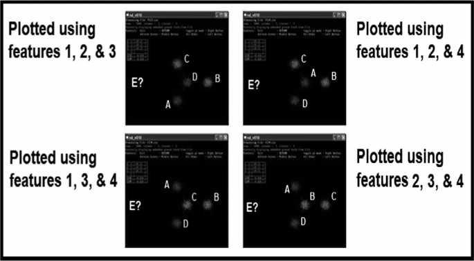

  

  Display the data in several projections to insure that something isn’t “lost” by leaving out a “good” dimension.

• 2. Plot the data in features 1, 2, and 4 (Fig. 3, upper-right plot)

• 3. Plot the data in features 1, 3, and 4 (Fig. 3, lower-left plot)

• 4. Plot the data in features 2, 3, and 4 (Fig. 3, lower-right plot)

No matter which of the four features is dropped, we obtain essentially the same view of the data, with the positions of the clusters permuted. But none of these views shows cluster E. Where is it?

If, instead of throwing away a feature, the data are viewed using one of the geometrically faithful N-dimensional visualizers in the data’s native 4-dimensional space, the presence of cluster E is immediately revealed: a fifth, coherent 1,000-point cluster that cannot be seen in any 3D feature-winnowing. For this data set, removal of any of the four features causes all class E vectors to be located at the center of one of the other classes. Not only has it become invisible, its class identity has been lost (Fig. 4).

Fig. 4.

Cluster E Cannot be seen in any lower-dimensional winnowing

No matter which subset of 1, 2, or 3 features is used to plot this data, the user will never see cluster E as a separate aggregation. From every 3D perspective, it is in the same place as one of the other three larger clusters and is obscured. However, In the data’s native 4-dimensional space, all five clusters are easily visible.

The phenomenon illustrated here happens in practice with real data; this kind of occlusion is often present to some degree in large, high-dimensional data sets. This is one of the things that makes pattern processing in these spaces difficult.

2.3 Parallel Coordinates (Inselberg Plots)

A 150+ year-old technique revived and extended by Alfred Inselberg beginning in 1959, Parallel coordinates retain all dimensions. To produce graphical displays, a separate vertical axis is used for each dimension. A feature vector is no longer a point in space, but a trace of end-to-end line segments across the display.

It is customary for the leftmost vertical axis to receive the first feature, then moving to the right for features 2 through N. Highly coherent clusters show up as bands of traces across the display.

Parallel coordinate plots have proven to be quite useful in applications. If each class of vectors is colorized, or plotted on a different horizontal axis, these plots provide an excellent method of looking for highly discriminating features. In Fig. 5, for example, class 1 is on the top plot, and class 2 is on the bottom plot. It is readily seen that features 5, 6, and 8 might be used to distinguish class 1 from class 2.

Fig. 5.

Parallel Coordinate plot of classes (CURRENT, ATTRIT)

Parallel coordinates, since they do not retain an intuitive analogy with the underlying data geometry require experience to interpret. The notions of cluster proximity, occlusion, shape, and spatial context are mostly lost.

3 Geometrically Intuitive Methods

Two methods will now be presented that the authors have formulated and applied to many real-world problems involving the visualization of discrete data (sets of feature vectors) having from 3 to 100 dimensions: Recursive Stereographic Projection (RSP), Tensor Projection (TP).

These methods render colorized graphical displays of high-dimensional discrete data that:

• are informative while remaining geometrically intuitive

• support on-screen data annotation (e.g., lasso clusters, pseudo-color visual artifacts)

• TP is fast enough that desktop machines can smoothly navigate 100-dimensional data sets having 50,000 points. RSP can smoothly navigate 20-dimensional data sets having 5,000 points.

• can stream data frames to disc to create movies of high-dimensional data sets in their native spaces tend to preserve geometric characteristics of the original high-dimensional data such as, occlusion, proximity, intersection, relative scale, spatial extent, shape, and coherence

3.1 Recursive Stereographic Projection (RSP)

As the name implies, Recursive Stereographic Projection (RSP) implements N-dimensional visualization using a recursive stereographic projection, a mathematical analogy between a sphere and a plane missing one point.

A positive real value r is chosen for the radii of the spheres by means of which the projections are done. The viewer is positioned at (r, 0, 0, …, 0).

Each down-projection follows the same pattern (Fig. 6):

Fig. 6.

Each projection to the next lower dimension is a projection from the normalized data on the surface of a ball, and the hyperplane beneath the ball. This is a one-point perspective projection, relative distances are scaled by how far they are from the viewer.

• A hyperplane to receive the projected data is perpendicular to the position vector of the viewer, and at distance equal to the r on the far side of the origin.

• All features vectors are z-scored coordinate-by-coordinate. Each vector is then normalized to length r. These two steps project the entire data set onto the N − 1 dimensional sphere centered at (r/2.0.0.,…0) having radius r/2. This places the data at the center of the display, which is where the algorithm maps the origin.

• The recursion proceeds by stereographically projecting each data point from the viewer location at the topmost point of the sphere onto a target hyperplane.

• Each projection reduces the dimension of the data by 1. The recursion is repeated on each data point until a set of two-dimensional data are obtained. This pair is plotted on the display as the location of the original point.

Visual navigation is accomplished by moving the feature vectors. For example, rotating a feature vector about the line (r, 0, 0, …, 0) is a fast matrix multiplication. In our implementation, this can be done on a laptop machine quickly enough to support smooth motion for 20 or fewer dimensions and 5,000 or fewer vectors. By repeating this operation using a small rotation angle, a “fly-around” survey of the data from various viewer perspectives is created.

As an example of the utility of this visualizer, consider the following application.

Work was underway on an important system for detecting and classifying opposing military vehicles from a distance of several miles. A sensor was developed to collect “signatures” from the vehicles so that human analysts, and eventually intelligent software, would be able to create catalogs of distant military threats so that the evolving posture of adversaries could be assessed in real-time.

Vehicle signatures were first collected at a test range. Sometimes the signatures were easy to match to vehicles, but there were quite a few instances for which dangerous offensive vehicles looked like trucks. Sending light armor to engage a “line of trucks” which turns out to be a column of tanks is a fatal mistake (Fig. 7).

Fig. 7.

Just how bad is the confusion between classes when this sensor is used? Exactly what is happening in the feature space that is leading to this problem?

In this instance, the use of N-dimensional visualization based upon RSP was used to view a 32-dimensional coding of the signature waveforms for a large number of test vehicles.

When visualized in its native 32-dimensional space, the signature data presents as three coherent, overlapping clusters. The “branch” at the upper left consists almost entirely of vectors of class1; the “branch” at the upper right consists almost entirely of vectors of class2. The clump at the bottom, consisting of about 25% of the data in even class proportions, is an unresolvable mixture (Fig. 8).

Fig. 8.

In 32-dimensional space, it was easy to see what was happening

Using this knowledge, we construct a classifier by segmenting the data using two perpendicular hyperplanes and labeling the bounded regions as in Fig. 8.

This classifier will have a classification accuracy of about 75% from the class1 and class2 regions, which are heterogeneous by class. Randomly assigning a class decision to points from the balanced mixture will be correct about 12.5% of the time, giving an overall classification accuracy on the training data of 87.5%

It is unlikely that a classifier would be built this way, but the value here is that it establishes the fact that any classifier that does not have a classification accuracy of at least 87.5% on this training set is inferior. Further, we knew that it would not be necessary to redesign the sensor (a massive expense) but could obtain reasonable performance with modest software tweaking.

3.2 Tensor Projection (TP)

For clarity, we pose an illustrative example (Fig. 9). Other instances are analogous.

Fig. 9.

This tensor product provides a parametric linear mapping from the feature space to R²

Consider the example of a 9-dimensional feature vector V = (f₁, f₂, …, f₉) in R⁹.

Let B = (b₁, b₂, b₃) and A = (a₁, a₂, a₃) be vectors of real parameters,

Form a tensor product to induce a mapping from R⁹ to R², where V → X = (x₁, x₂):

To render the vector V in R9 on a flat display, we plot (x1, x2).

In general, given a feature vector W = (w₁, w₂, …, w_m) in R^M, we form a tensor product as above:

• Begin with the N-by-N identity matrix I_N, where N is the smallest perfect square ≥ M. Set K = √N.

• load W into I_N in some standard order (we use row-major order).

• Select at parameter vector B in R^K and creating two rows as above with the top row having 0 in the even positions, and the bottom row having 0 in the odd positions, with the coordinates of B interleaved as above. (Exactly how this interleaving is chosen is somewhat arbitrary, of course).

• Select parameter vector A in R^K, place it into the column vector to the right of I_N.

• Plot the resulting tensor product (x₁, x₂) for W.

The coordinates of A and B provide parameters that the user can manipulate to modify the mapping for feedback in real time.

The TP high-dimensional visualization creates geometrically faithful views of data points as they actually reside in their high-dimensional space. Nearness, occlusion, and perspective are preserved.

We have implemented the GUI concept depicted in Fig. 10.

Fig. 10.

TP allows on-screen scaling of coordinates so that clusters can be easily identified

Initially, all the data are at the center of the display, because all parameters are set to 0.

The boxes at the upper left-hand corner of the large rectangular display box have a blue boundary. These are the transformation parameter controls (a₁, a₂, etc.). The white line is “zero”; values above the white line are positive, and values below the white line are negative.

The last (rightmost) bar is the “zoom” bar. It allows you to zoom in or out of the central region of the display. A negative zoom value will produce a mirror image of the corresponding positive zoom value.

Holding down the left mouse button, the user drags a transformation parameter color bar up and down. This sets the corresponding transformation parameter. Different parameter values give different projections of the feature data, changing the display accordingly, in real-time.

The boxes along the upper right-hand corner of the large rectangular display box have a red boundary. These are the navigation parameter controls (b₁, b₂, etc.). For all but the bottom bar, the white line is “zero”; values to the right of the white line are positive, and values to the left of the white line are negative.

This positive-negative paradigm does not apply to the bottom bar. The last (bottommost) bar is the “icon size” bar. It allows you to change the size of the icons used to represent data points. The values range from 0 (1 pixel) to a maximum positive radius.

Holding down the left mouse button, the user drags a navigation parameter color bar left and right. This sets the corresponding navigation parameter. Different parameter values effectively allow you to view the data from different locations, changing the display accordingly, in real-time.

Figure 10 is a screen shot of an implementation of a TP display after loading a file containing 100 clusters each consisting of 20 points in a 100-dimensional space. The clusters are plainly visible, and intuitive. What can’t be seen on this screen-shot is the fact that TP allows the user to rotate and “flex” the data in various ways, zoom, change the icon size, and save lower dimensional representations of the data.

Dimension reduction for visualization produces successively lower-dimensional representations of the data, which can be saved for analysis or as feature winnowing products.

As an example of the utility of this visualizer, consider the following application.

Face-to-face interactions among groups of people follow certain conventions. These conventions provide an orderly structure for effective communication. This results in the formation of a variety of associations/relationships, such as “cliques”, as people gather around and/or disperse driven by interests, demographics, and goals. These associations have been studied extensively, and analysis of the resulting social structures can be used to characterize the interests, goals, and even personalities of those involved.

Interactions among the participants on social media platforms also give rise to complex social structures, which are the basis of social engineering, forensic data mining, and behavior analysis.

When viewed graphically, certain types of social media interaction become immediately apparent: cliques can be analyzed visually, complex interactions that would otherwise defy detection can be seen, and forecasting and planning are enhanced. In particular, visualization of high-dimensional social media structures can be used to support profiling for marketing products, assessing and influencing public opinion, and estimating malware risk and susceptibility.

FACT: Human and BOT behaviors often look very different in this type of visualization.

A large collection of social media posts was numericized using text processing techniques. The resulting feature space was then visualized using the TP visualizer, showing a clear difference between BOT behaviors and human behaviors on this social media platform. This has phenomenon has since been observed visually in this way on other social media platforms (Fig. 11).

Fig. 11.

The lack of diversity of a wide variety of BOTS is clearly seen in this 10-dimensional space

4 Future Work

• Build a user interface, allowing users to interact with the machine space. Functionality would include zooming in and out and spin the sphere to discover the range of solutions for the machine. Allow the user to manually “game” the coloration: adjusting the color boundaries of the model by accuracy to see how accurate a machine can get before it is not efficient.

• Use described visual methods not just for forensics, but for design as well. In an interface similar to the one described above, a user could be given the ability to select a machine by mouse click.

• Optimize the rendering process for speed to support direct user interaction.

• Additional cross-paradigm experimentation using other reasoning paradigms, such as Self Organizing Maps.

• Use for analysis of known pathologies (such as local extrema).

References

Appel, A.: Some techniques for shading machine renderings of solids. In: Proceedings of AFIPS JSCC, vol. 32, pp. 37–45 (1968)
Delmater, R., Hancock, M.: Data Mining Explained, pp. 145–146. Digital Press (2001)
Acknowledgments
The authors would like to thank the Sirius Project for facilitating this research.
Author information
Authors and Affiliations
Corresponding authors
Editor information
Editors and Affiliations
Rights and permissions
Copyright information
© 2019 Springer Nature Switzerland AG
About this paper
Cite this paper
Hancock, M. et al. (2019). Geometrically Intuitive Rendering of High-Dimensional Data. In: Schmorrow, D., Fidopiastis, C. (eds) Augmented Cognition. HCII 2019. Lecture Notes in Computer Science(), vol 11580. Springer, Cham. https://doi.org/10.1007/978-3-030-22419-6_16
Download citation
DOI: https://doi.org/10.1007/978-3-030-22419-6_16
Published:
Publisher Name: Springer, Cham
Print ISBN: 978-3-030-22418-9
Online ISBN: 978-3-030-22419-6
eBook Packages: Computer ScienceComputer Science (R0)