
Getting Acquainted with the Fractional Laplacian

  • Chapter
  • First Online:
Contemporary Research in Elliptic PDEs and Related Topics

Part of the book series: Springer INdAM Series ((SINDAMS,volume 33))

Abstract

These are the handouts of an undergraduate minicourse at the Università di Bari (see Fig. 1), in the context of the 2017 INdAM Intensive Period “Contemporary Research in elliptic PDEs and related topics”. Without any intention to serve as a throughout epitome to the subject, we hope that these notes can be of some help for a very initial introduction to a fascinating field of classical and modern research.

This is a preview of subscription content, log in via an institution to check access.

Access this chapter

Chapter
USD 29.95
Price excludes VAT (USA)
  • Available as PDF
  • Read on any device
  • Instant download
  • Own it forever
eBook
USD 44.99
Price excludes VAT (USA)
  • Available as EPUB and PDF
  • Read on any device
  • Instant download
  • Own it forever
Softcover Book
USD 59.99
Price excludes VAT (USA)
  • Compact, lightweight edition
  • Dispatched in 3 to 5 business days
  • Free shipping worldwide - see info
Hardcover Book
USD 59.99
Price excludes VAT (USA)
  • Durable hardcover edition
  • Dispatched in 3 to 5 business days
  • Free shipping worldwide - see info

Tax calculation will be finalised at checkout

Purchases are for personal use only

Institutional subscriptions

〈〈The longest appendix measured 26cm (10.24in) when it was removed from 72-year-old Safranco August (Croatia) during an autopsy at the Ljudevit Jurak University Department of Pathology, Zagreb, Croatia, on 26 August 2006.〉〉

(Source: http://www.guinnessworldrecords.com/world-records/largest-appendix-removed)

Notes

  1. 1.

    The notion (or, better to say, several possible notions) of fractional derivatives attracted the attention of many distinguished mathematicians, such as Leibniz, Bernoulli, Euler, Fourier, Abel, Liouville, Riemann, Hadamard and Riesz, among the others. A very interesting historical outline is given in pages xxvii–xxxvi of [104].

  2. 2.

    We think that it is quite remarkable that the operator obtained by the inverse Fourier Transform of \( \,|\xi |{ }^{2} \,\widehat u\), the classical Laplacian, reduces to a local operator. This is not true for the inverse Fourier Transform of \( \,|\xi |{ }^{2s} \,\widehat u\). In this spirit, it is interesting to remark that the fact that the classical Laplacian is a local operator is not immediate from its definition in Fourier space, since computing Fourier Transforms is always a nonlocal operation.

  3. 3.

    Some care has to be used with extension methods, since the solution of (2.6) is not unique (if U solves (2.6), then so does U(x, y) + cy for any \(c\in \mathbb {R}\)). The “right” solution of (2.6) that one has to take into account is the one with “decay at infinity”, or belonging to an “energy space”, or obtained by convolution with a Poisson-type kernel. See e.g. [24] for details.

    Also, the extension method in (2.6) and (2.7) can be related to an engineering application of the fractional Laplacian motivated by the displacement of elastic membranes on thin (i.e. codimension one) obstacles, see [28]. The intuition for such application can be grasped from Figs. 7, 10, and 12. These pictures can be also useful to develop some intuition about extension methods for fractional operators and boundary reaction-diffusion equations.

  4. 4.

    See Appendix A in [103] for a very nice explanation of the dimensional analysis and for a throughout discussion of its role in detecting fundamental solutions.

  5. 5.

    Some colleagues pointed out to us that the use of R and r in some steps of formula (5.5) of [54] are inadequate. We take this opportunity to amend such a flaw, presenting a short proof of (5.5) of [54]. Given ε > 0, we notice that

    where the constants are also allowed to depend on Ω and u. Furthermore, if we define Ωε to be the set of all the points in Ω with distance less than ε from  Ω, the regularity of  Ω implies that the measure of Ωε is bounded by const ε, and therefore

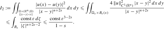
    These observations imply that

    Taking ε as small as we wish, we obtain formula (5.5) in [54].

  6. 6.

    From the geometric point of view, one can also take radial coordinates, compute the derivatives of K along the unit sphere and use scaling.

  7. 7.

    The difficulty in proving (G.1) is that the function u 1∕2 is not differentiable at ± 1 and the derivative taken inside the integral might produce a singularity (in fact, formula (G.1) exactly says that such derivative can be performed with no harm inside the integral). The reader who is already familiar with the basics of functional analysis can prove (G.1) by using the theory of absolutely continuous functions, see e.g. Theorem 8.21 in [98]. We provide here a direct proof, available to everybody.

  8. 8.

    As a historical remark, we recall that e −|ξ| is sometimes called the “Abel Kernel” and its Fourier Transform the “Poisson Kernel”, which in dimension 1 reduces to the “Cauchy-Lorentz, or Breit-Wigner, Distribution” (that has also classical geometric interpretations as the “Witch of Agnesi”, and so many names attached to a single function clearly demonstrate its importance in numerous applications).

  9. 9.

    Let us mention another conceptual simplification of nonlocal problems: in this setting, the integral representation often allows the formulation of problems with minimal requirements on the functions involved (such as measurability and possibly minor pointwise or integral bounds). Conversely, in the classical setting, even to just formulate a problem, one often needs assumptions and tools from functional analysis, comprising e.g. Sobolev differentiability, distributions or functions of bounded variations.

  10. 10.

    In complex variables, one can also interpret the function U in terms of the principal argument function

    $$\displaystyle \begin{aligned}{\mathrm{Arg}}(r e^{i\varphi})=\varphi\in(-\pi,\pi],\end{aligned}$$

    with branch cut along the nonpositive real axis. Notice indeed that, if z = x + iy and y > 0,

    $$\displaystyle \begin{aligned}{\mathrm{Arg}}(z+i)=\frac\pi2-\arctan\frac{x}{y+1}=\frac\pi2\left(1-U(x,y) \right).\end{aligned}$$

    This observation would also lead to (L.1).

  11. 11.

    The representation in (P.2) makes sense for a larger class of functions with respect to (2.51), so in a sense (P.2) can be interpreted as an extension of definition (2.51).

  12. 12.

    A slightly different approach as that in (3.7) is to consider the energy functional in (3.9) and prove, e.g. by Taylor expansion, that it converges to the energy functional

    $$\displaystyle \begin{aligned}\,{\mathrm{const}}\, \int_{\mathbb{R}^n}a_{ij}(x) \,\partial_i u(x)\,\partial_j u(x)\,dx.\end{aligned}$$

    On the other hand, a different proof of (3.7), that was nicely pointed out to us by Jonas Hirsch (who has also acted as a skilled cartoonist for Fig. 13) after a lecture, can be performed by taking into account the weak form of the operator in (3.5), i.e. integrating such expression against a test function \(\varphi \in C^\infty _0(\mathbb {R}^n)\), thus finding

    $$\displaystyle \begin{aligned} \begin{array}{rcl} &\displaystyle &\displaystyle (1-s)\,\iint_{\mathbb{R}^n\times\mathbb{R}^n} \frac{ \big(u(x)-u(x-y)\big)\,\varphi(x)}{ |M(x-y,y)\, y|{}^{n+2s}}\,dx\,dy \\ &\displaystyle =&\displaystyle (1-s)\,\iint_{\mathbb{R}^n\times\mathbb{R}^n} \frac{ \big(u(x)-u(z)\big)\,\varphi(x)}{ |M(z,x-z)\,(x-z)|{}^{n+2s}}\,dx\,dz \\ \noalign{} &\displaystyle =&\displaystyle (1-s)\,\iint_{\mathbb{R}^n\times\mathbb{R}^n} \frac{ \big(u(z)-u(x)\big)\,\varphi(z)}{ |M(x,z-x)\,(x-z)|{}^{n+2s}}\,dx\,dz \\ &\displaystyle =&\displaystyle -(1-s)\,\iint_{\mathbb{R}^n\times\mathbb{R}^n} \frac{ \big(u(x)-u(z)\big)\,\varphi(z)}{ |M(z,x-z)\,(x-z)|{}^{n+2s}}\,dx\,dz ,\end{array} \end{aligned} $$

    where the structural condition (3.6) has been used in the last line. This means that the weak formulation of the operator in (3.5) can be written as

    $$\displaystyle \begin{aligned}\frac{1-s}{2}\,\iint_{\mathbb{R}^n\times\mathbb{R}^n} \frac{ \big(u(x)-u(z)\big)\,\big(\varphi(x)-\varphi(z)\big)}{ |M(z,x-z)\,(x-z)|{}^{n+2s}}\,dx\,dz.\end{aligned}$$

    So one can expand this expression and take the limit as , to obtain

    $$\displaystyle \begin{aligned}\,{\mathrm{const}}\, \int_{\mathbb{R}^n}a_{ij}(x) \,\partial_i u(x)\,\partial_j\varphi(x)\,dx,\end{aligned}$$

    which is indeed the weak formulation of the classical divergence form operator.

References

  1. N. Abatangelo, Large s-harmonic functions and boundary blow-up solutions for the fractional Laplacian. Discrete Contin. Dyn. Syst. 35(12), 5555–5607 (2015). https://doi.org/10.3934/dcds.2015.35.5555. MR3393247

    Article  MathSciNet  MATH  Google Scholar 

  2. N. Abatangelo, L. Dupaigne, Nonhomogeneous boundary conditions for the spectral fractional Laplacian. Ann. Inst. H. Poincaré Anal. Non Linéaire 34(2), 439–467 (2017). https://doi.org/10.1016/j.anihpc.2016.02.001. MR3610940

    Article  MathSciNet  MATH  Google Scholar 

  3. N. Abatangelo, S. Jarohs, A. Saldaña, Positive powers of the Laplacian: from hypersingular integrals to boundary value problems. Commun. Pure Appl. Anal. 17(3), 899–922 (2018). https://doi.org/10.3934/cpaa.2018045. MR3809107

    Article  MathSciNet  MATH  Google Scholar 

  4. N. Abatangelo, S. Jarohs, A. Saldaña, Green function and Martin kernel for higher-order fractional Laplacians in balls. Nonlinear Anal. 175, 173–190 (2018). https://doi.org/10.1016/j.na.2018.05.019. MR3830727

    Article  MathSciNet  MATH  Google Scholar 

  5. N. Abatangelo, S. Jarohs, A. Saldaña, On the loss of maximum principles for higher-order fractional Laplacians. Proc. Am. Math. Soc. 146(11), 4823–4835 (2018). https://doi.org/10.1090/proc/14165. MR3856149

    Article  MathSciNet  MATH  Google Scholar 

  6. E. Affili, S. Dipierro, E. Valdinoci, Decay estimates in time for classical and anomalous diffusion. arXiv e-prints (2018), available at 1812.09451

    Google Scholar 

  7. M. Allen, L. Caffarelli, A. Vasseur, A parabolic problem with a fractional time derivative. Arch. Ration. Mech. Anal. 221(2), 603–630 (2016). https://doi.org/10.1007/s00205-016-0969-z. MR3488533

    Article  MathSciNet  MATH  Google Scholar 

  8. F. Andreu-Vaillo, J.M. Mazón, J.D. Rossi, J.J. Toledo-Melero, Nonlocal Diffusion Problems, Mathematical Surveys and Monographs, vol. 165 (American Mathematical Society, Providence, 2010); Real Sociedad Matemática Española, Madrid, 2010. MR2722295

    Google Scholar 

  9. D. Applebaum, Lévy Processes and Stochastic Calculus. Cambridge Studies in Advanced Mathematics, 2nd edn., vol. 116 (Cambridge University Press, Cambridge, 2009). MR2512800

  10. V.E. Arkhincheev, É.M. Baskin, Anomalous diffusion and drift in a comb model of percolation clusters. J. Exp. Theor. Phys. 73, 161–165 (1991)

    Google Scholar 

  11. A.V. Balakrishnan, Fractional powers of closed operators and the semigroups generated by them. Pac. J. Math. 10, 419–437 (1960). MR0115096

    MathSciNet  Google Scholar 

  12. R. Bañuelos, K. Bogdan, Lévy processes and Fourier multipliers. J. Funct. Anal. 250(1), 197–213 (2007). https://doi.org/10.1016/j.jfa.2007.05.013. MR2345912

    Article  MathSciNet  MATH  Google Scholar 

  13. B. Barrios, I. Peral, F. Soria, E. Valdinoci, A Widder’s type theorem for the heat equation with nonlocal diffusion. Arch. Ration. Mech. Anal. 213(2), 629–650 (2014). https://doi.org/10.1007/s00205-014-0733-1. MR3211862

    Article  MathSciNet  MATH  Google Scholar 

  14. R.F. Bass, D.A. Levin, Harnack inequalities for jump processes. Potential Anal. 17(4), 375–388 (2002). https://doi.org/10.1023/A:1016378210944. MR1918242

    Article  MathSciNet  Google Scholar 

  15. A. Bendikov, Asymptotic formulas for symmetric stable semigroups. Expo. Math. 12(4), 381–384 (1994). MR1297844

  16. J. Bertoin, Lévy Processes. Cambridge Tracts in Mathematics, vol. 121 (Cambridge University Press, Cambridge, 1996). MR1406564

  17. R.M. Blumenthal, R.K. Getoor, Some theorems on stable processes. Trans. Am. Math. Soc. 95, 263–273 (1960). https://doi.org/10.2307/1993291. MR0119247

    Article  MathSciNet  MATH  Google Scholar 

  18. K. Bogdan, T. Byczkowski, Potential theory for the α-stable Schrödinger operator on bounded Lipschitz domains. Stud. Math. 133(1), 53–92 (1999). MR1671973

  19. K. Bogdan, T. Żak, On Kelvin transformation. J. Theor. Probab. 19(1), 89–120 (2006). MR2256481

  20. M. Bonforte, A. Figalli, J.L. Vázquez, Sharp global estimates for local and nonlocal porous medium-type equations in bounded domains. Anal. PDE 11(4), 945–982 (2018). https://doi.org/10.2140/apde.2018.11.945. MR3749373

    Article  MathSciNet  MATH  Google Scholar 

  21. L. Brasco, S. Mosconi, M. Squassina, Optimal decay of extremals for the fractional Sobolev inequality. Calc. Var. Partial Differ. Equ. 55(2), 23, 32 (2016). https://doi.org/10.1007/s00526-016-0958-y. MR3461371

  22. C. Bucur, Some observations on the Green function for the ball in the fractional Laplace framework. Commun. Pure Appl. Anal. 15(2), 657–699 (2016). https://doi.org/10.3934/cpaa.2016.15.657. MR3461641

  23. C. Bucur, Local density of Caputo-stationary functions in the space of smooth functions. ESAIM Control Optim. Calc. Var. 23(4), 1361–1380 (2017). https://doi.org/10.1051/cocv/2016056. MR3716924

    MathSciNet  MATH  Google Scholar 

  24. C. Bucur, E. Valdinoci, Nonlocal Diffusion and Applications. Lecture Notes of the Unione Matematica Italiana, vol. 20 (Springer, Cham, 2016); Unione Matematica Italiana, Bologna. MR3469920

  25. C. Bucur, L. Lombardini, E. Valdinoci, Complete stickiness of nonlocal minimal surfaces for small values of the fractional parameter. Ann. Inst. H. Poincaré Anal. Non Linéaire 36(3), 655–703 (2019)

    Article  MathSciNet  MATH  Google Scholar 

  26. X. Cabré, M. Cozzi, A gradient estimate for nonlocal minimal graphs. Duke Math. J. 168(5), 775–848 (2019)

    Article  MathSciNet  MATH  Google Scholar 

  27. X. Cabré, Y. Sire, Nonlinear equations for fractional Laplacians II: existence, uniqueness, and qualitative properties of solutions. Trans. Am. Math. Soc. 367(2), 911–941 (2015). https://doi.org/10.1090/S0002-9947-2014-05906-0. MR3280032

    Article  MathSciNet  MATH  Google Scholar 

  28. L.A. Caffarelli, Further regularity for the Signorini problem. Commun. Partial Differ. Equ. 4(9), 1067–1075 (1979). https://doi.org/10.1080/03605307908820119. MR542512

    Article  MathSciNet  MATH  Google Scholar 

  29. L. Caffarelli, F. Charro, On a fractional Monge-Ampère operator. Ann. PDE 1(1), 4, 47 (2015). MR3479063

  30. L. Caffarelli, L. Silvestre, An extension problem related to the fractional Laplacian. Commun. Partial Differ. Equ. 32(7–9), 1245–1260 (2007). https://doi.org/10.1080/03605300600987306. MR2354493

    Article  MathSciNet  MATH  Google Scholar 

  31. L. Caffarelli, L. Silvestre, Regularity theory for fully nonlinear integro-differential equations. Commun. Pure Appl. Math. 62(5), 597–638 (2009). MR2494809

  32. L. Caffarelli, L. Silvestre, Hölder regularity for generalized master equations with rough kernels, in Advances in Analysis: The Legacy of Elias M. Stein. Princeton Mathematical Series, vol. 50 (Princeton University Press, Princeton, 2014), pp. 63–83. MR3329847

  33. L.A. Caffarelli, J.L. Vázquez, Asymptotic behaviour of a porous medium equation with fractional diffusion. Discrete Contin. Dyn. Syst. 29(4), 1393–1404 (2011). MR2773189

  34. L. Caffarelli, F. Soria, J.L. Vázquez, Regularity of solutions of the fractional porous medium flow. J. Eur. Math. Soc. (JEMS) 15(5), 1701–1746 (2013). https://doi.org/10.4171/JEMS/401. MR3082241

    Article  MathSciNet  MATH  Google Scholar 

  35. M. Caputo, Linear models of dissipation whose Q is almost frequency independent. II. Fract. Calc. Appl. Anal. 11(1), 4–14 (2008). Reprinted from Geophys. J. R. Astr. Soc. 13(1967), no. 5, 529–539. MR2379269

    MathSciNet  MATH  Google Scholar 

  36. A. Carbotti, S. Dipierro, E. Valdinoci, Local Density of Solutions to Fractional Equations. Graduate Studies in Mathematics (De Gruyter, Berlin, 2019)

    Google Scholar 

  37. A. Carbotti, S. Dipierro, E. Valdinoci, Local density of Caputo-stationary functions of any order. Complex Var. Elliptic Equ. (to appear). https://doi.org/10.1080/17476933.2018.1544631

  38. R. Carmona, W.C. Masters, B. Simon, Relativistic Schrödinger operators: asymptotic behavior of the eigenfunctions. J. Funct. Anal. 91(1), 117–142 (1990). https://doi.org/10.1016/0022-1236(90)90049-Q. MR1054115

    Article  MathSciNet  MATH  Google Scholar 

  39. A. Cesaroni, M. Novaga, Symmetric self-shrinkers for the fractional mean curvature flow. ArXiv e-prints (2018), available at 1812.01847

    Google Scholar 

  40. A. Cesaroni, S. Dipierro, M. Novaga, E. Valdinoci, Fattening and nonfattening phenomena for planar nonlocal curvature flows. Math. Ann. (to appear). https://doi.org/10.1007/s00208-018-1793-6

  41. E. Cinti, C. Sinestrari, E. Valdinoci, Neckpinch singularities in fractional mean curvature flows. Proc. Am. Math. Soc. 146(6), 2637–2646 (2018). https://doi.org/10.1090/proc/14002. MR3778164

    Article  MathSciNet  MATH  Google Scholar 

  42. E. Cinti, J. Serra, E. Valdinoci, Quantitative flatness results and BV-estimates for stable nonlocal minimal surfaces. J. Differ. Geom. (to appear)

    Google Scholar 

  43. J. Coville, Harnack type inequality for positive solution of some integral equation. Ann. Mat. Pura Appl. 191(3), 503–528 (2012). https://doi.org/10.1007/s10231-011-0193-2. MR2958346

    Article  MathSciNet  MATH  Google Scholar 

  44. J.C. Cox, The valuation of options for alternative stochastic processes. J. Finan. Econ. 3(1–2), 145–166 (1976). https://doi.org/10.1016/0304-405X(76)90023-4

    Article  Google Scholar 

  45. M. Cozzi, E. Valdinoci, On the growth of nonlocal catenoids. Atti Accad. Naz. Lincei Rend. Lincei Mat. Appl. (to appear)

    Google Scholar 

  46. J. Dávila, M. del Pino, J. Wei, Nonlocal s-minimal surfaces and Lawson cones. J. Differ. Geom. 109(1), 111–175 (2018). https://doi.org/10.4310/jdg/1525399218. MR3798717

    Article  MathSciNet  MATH  Google Scholar 

  47. C.-S. Deng, R.L. Schilling, Exact Asymptotic Formulas for the Heat Kernels of Space and Time-Fractional Equations, ArXiv e-prints (2018), available at 1803.11435

    Google Scholar 

  48. A. de Pablo, F. Quirós, A. Rodríguez, J.L. Vázquez, A fractional porous medium equation. Adv. Math. 226(2), 1378–1409 (2011). https://doi.org/10.1016/j.aim.2010.07.017. MR2737788

    Article  MathSciNet  MATH  Google Scholar 

  49. E. Di Nezza, G. Palatucci, E. Valdinoci, Hitchhiker’s guide to the fractional Sobolev spaces. Bull. Sci. Math. 136(5), 521–573 (2012). https://doi.org/10.1016/j.bulsci.2011.12.004. MR2944369

    Article  MathSciNet  MATH  Google Scholar 

  50. S. Dipierro, H.-C. Grunau, Boggio’s formula for fractional polyharmonic Dirichlet problems. Ann. Mat. Pura Appl. 196(4), 1327–1344 (2017). https://doi.org/10.1007/s10231-016-0618-z. MR3673669

    Article  MathSciNet  MATH  Google Scholar 

  51. S. Dipierro, E. Valdinoci, A simple mathematical model inspired by the Purkinje cells: from delayed travelling waves to fractional diffusion. Bull. Math. Biol. 80(7), 1849–1870 (2018). https://doi.org/10.1007/s11538-018-0437-z. MR3814763

    Article  MathSciNet  MATH  Google Scholar 

  52. S. Dipierro, G. Palatucci, E. Valdinoci, Dislocation dynamics in crystals: a macroscopic theory in a fractional Laplace setting. Commun. Math. Phys. 333(2), 1061–1105 (2015). https://doi.org/10.1007/s00220-014-2118-6. MR3296170

    Article  MathSciNet  MATH  Google Scholar 

  53. S. Dipierro, O. Savin, E. Valdinoci, Graph properties for nonlocal minimal surfaces. Calc. Var. Partial Differ. Equ. 55(4), 86, 25 (2016). https://doi.org/10.1007/s00526-016-1020-9. MR3516886

  54. S. Dipierro, X. Ros-Oton, E. Valdinoci, Nonlocal problems with Neumann boundary conditions. Rev. Mat. Iberoam. 33(2), 377–416 (2017). https://doi.org/10.4171/RMI/942. MR3651008

    Article  MathSciNet  MATH  Google Scholar 

  55. S. Dipierro, O. Savin, E. Valdinoci, All functions are locally s-harmonic up to a small error. J. Eur. Math. Soc. (JEMS) 19(4), 957–966 (2017). https://doi.org/10.4171/JEMS/684. MR3626547

    Article  MathSciNet  MATH  Google Scholar 

  56. S. Dipierro, O. Savin, E. Valdinoci, Boundary behavior of nonlocal minimal surfaces. J. Funct. Anal. 272(5), 1791–1851 (2017). https://doi.org/10.1016/j.jfa.2016.11.016. MR3596708

    Article  MathSciNet  MATH  Google Scholar 

  57. S. Dipierro, N. Soave, E. Valdinoci, On stable solutions of boundary reaction-diffusion equations and applications to nonlocal problems with Neumann data. Indiana Univ. Math. J. 67(1), 429–469 (2018). https://doi.org/10.1512/iumj.2018.67.6282. MR3776028

    Article  MathSciNet  MATH  Google Scholar 

  58. S. Dipierro, O. Savin, E. Valdinoci, Local approximation of arbitrary functions by solutions of nonlocal equations. J. Geom. Anal. 29(2), 1428–1455 (2019)

    Article  MathSciNet  MATH  Google Scholar 

  59. S. Dipierro, O. Savin, E. Valdinoci, Definition of fractional Laplacian for functions with polynomial growth. Rev. Mat. Iberoam (to appear)

    Google Scholar 

  60. S. Dipierro, J. Serra, E. Valdinoci, Improvement of flatness for nonlocal phase transitions. Amer. J. Math. (to appear)

    Google Scholar 

  61. B. Dyda, Fractional calculus for power functions and eigenvalues of the fractional Laplacian. Fract. Calc. Appl. Anal. 15(4), 536–555 (2012). https://doi.org/10.2478/s13540-012-0038-8. MR2974318

  62. L.C. Evans, Partial Differential Equations. Graduate Studies in Mathematics, vol. 19 (American Mathematical Society, Providence, 1998). MR1625845

  63. M.M. Fall, T. Weth, Nonexistence results for a class of fractional elliptic boundary value problems. J. Funct. Anal. 263(8), 2205–2227 (2012). https://doi.org/10.1016/j.jfa.2012.06.018. MR2964681

    Article  MathSciNet  MATH  Google Scholar 

  64. M.M. Fall, T. Weth, Liouville theorems for a general class of nonlocal operators. Potential Anal. 45(1), 187–200 (2016). https://doi.org/10.1007/s11118-016-9546-1. MR3511811

    Article  MathSciNet  MATH  Google Scholar 

  65. A. Farina, E. Valdinoci, The state of the art for a conjecture of De Giorgi and related problems, in Recent Progress on Reaction-Diffusion Systems and Viscosity Solutions (World Scientific Publishing, Hackensack, 2009), pp. 74–96. https://doi.org/10.1142/9789812834744_0004. MR2528756

  66. P. Felmer, A. Quaas, Boundary blow up solutions for fractional elliptic equations. Asymptot. Anal. 78(3), 123–144 (2012). MR2985500

  67. A. Figalli, J. Serra, On stable solutions for boundary reactions: a De Giorgi-type result in dimension 4 + 1, preprint at arXiv:1705.02781 (2017, submitted)

    Google Scholar 

  68. R.L. Frank, E. Lenzmann, L. Silvestre, Uniqueness of radial solutions for the fractional Laplacian. Commun. Pure Appl. Math. 69(9), 1671–1726 (2016). https://doi.org/10.1002/cpa.21591. MR3530361

    Article  MathSciNet  MATH  Google Scholar 

  69. R.K. Getoor, First passage times for symmetric stable processes in space. Trans. Am. Math. Soc. 101, 75–90 (1961). https://doi.org/10.2307/1993412. MR0137148

    Article  MathSciNet  MATH  Google Scholar 

  70. T. Ghosh, M. Salo, G. Uhlmann, The Calderón problem for the fractional Schrödinger equation. ArXiv e-prints (2016), available at 1609.09248

    Google Scholar 

  71. D. Gilbarg, N.S. Trudinger, Elliptic Partial Differential Equations of Second Order. Classics in Mathematics (Springer, Berlin, 2001). Reprint of the 1998 edition. MR1814364

  72. E. Giusti, Direct Methods in the Calculus of Variations (World Scientific Publishing, River Edge, 2003). MR1962933

    Book  Google Scholar 

  73. Q. Han, F. Lin, Elliptic Partial Differential Equations. Courant Lecture Notes in Mathematics, 2nd edn., vol. 1 (Courant Institute of Mathematical Sciences/American Mathematical Society, New York/Providence, 2011). MR2777537

  74. N. Jacob, Pseudo-Differential Operators and Markov Processes. Mathematical Research, vol. 94 (Akademie Verlag, Berlin, 1996). MR1409607

  75. M. Kaßmann, Harnack-Ungleichungen Für nichtlokale Differentialoperatoren und Dirichlet-Formen (in German). Bonner Mathematische Schriften [Bonn Mathematical Publications], vol. 336 (Universität Bonn, Mathematisches Institut, Bonn, 2001). Dissertation, Rheinische Friedrich-Wilhelms-Universität Bonn, Bonn, 2000. MR1941020

  76. M. Kaßmann, A new formulation of Harnack’s inequality for nonlocal operators. C. R. Math. Acad. Sci. Paris 349(11–12), 637–640 (2011). https://doi.org/10.1016/j.crma.2011.04.014 (English, with English and French summaries). MR2817382

    Article  MathSciNet  MATH  Google Scholar 

  77. M. Kaßmann, Jump processes and nonlocal operators, in Recent Developments in Nonlocal Theory (De Gruyter, Berlin, 2018), pp. 274–302. MR3824215

  78. V. Kolokoltsov, Symmetric stable laws and stable-like jump-diffusions. Proc. Lond. Math. Soc. 80(3), 725–768 (2000). https://doi.org/10.1112/S0024611500012314. MR1744782

    Article  MathSciNet  MATH  Google Scholar 

  79. N.V. Krylov, On the paper “All functions are locally s-harmonic up to a small error” by Dipierro, Savin, and Valdinoci. ArXiv e-prints (2018), available at 1810.07648

    Google Scholar 

  80. T. Kuusi, G. Mingione, Y. Sire, Nonlocal equations with measure data. Commun. Math. Phys. 337(3), 1317–1368 (2015). https://doi.org/10.1007/s00220-015-2356-2. MR3339179

    Article  MathSciNet  MATH  Google Scholar 

  81. M. Kwaśnicki, Ten equivalent definitions of the fractional Laplace operator. Fract. Calc. Appl. Anal. 20(1), 7–51 (2017). https://doi.org/10.1515/fca-2017-0002. MR3613319

  82. N.S. Landkof, Foundations of Modern Potential Theory (Springer, New York, 1972). Translated from the Russian by A. P. Doohovskoy; Die Grundlehren der mathematischen Wissenschaften, Band 180. MR0350027

  83. H.C. Lara, G. Dávila, Regularity for solutions of non local parabolic equations. Calc. Var. Partial Differ. Equ. 49(1–2), 139–172 (2014). https://doi.org/10.1007/s00526-012-0576-2. MR3148110

  84. F. Mainardi, Fractional Calculus and Waves in Linear Viscoelasticity (Imperial College Press, London, 2010). An introduction to mathematical models. MR2676137

  85. F. Mainardi, Y. Luchko, G. Pagnini, The fundamental solution of the space-time fractional diffusion equation. Fract. Calc. Appl. Anal. 4(2), 153–192 (2001). MR1829592

  86. F. Mainardi, P. Paradisi, R. Gorenflo, Probability distributions generated by fractional diffusion equations. preprint at arXiv:0704.0320v1 (2007, submitted)

    Google Scholar 

  87. B. Mandelbrot, The variation of certain speculative prices. J. Bus. 36, 394 (1963)

    Article  Google Scholar 

  88. J.M. Mazón, J.D. Rossi, J. Toledo, The heat content for nonlocal diffusion with non-singular kernels. Adv. Nonlinear Stud. 17(2), 255–268 (2017). https://doi.org/10.1515/ans-2017-0005. MR3641640

  89. R. Metzler, J. Klafter, The restaurant at the end of the random walk: recent developments in the description of anomalous transport by fractional dynamics. J. Phys. A 37(31), R161–R208 (2004). https://doi.org/10.1088/0305-4470/37/31/R01. MR2090004

    Article  MathSciNet  MATH  Google Scholar 

  90. E. Montefusco, B. Pellacci, G. Verzini, Fractional diffusion with Neumann boundary conditions: the logistic equation. Discrete Contin. Dyn. Syst. Ser. B 18(8), 2175–2202 (2013). https://doi.org/10.3934/dcdsb.2013.18.2175. MR3082317

    Article  MathSciNet  MATH  Google Scholar 

  91. R. Musina, A.I. Nazarov, On fractional Laplacians. Commun. Partial Differ. Equ. 39(9), 1780–1790 (2014). https://doi.org/10.1080/03605302.2013.864304. MR3246044

    Article  MathSciNet  MATH  Google Scholar 

  92. G. Palatucci, O. Savin, E. Valdinoci, Local and global minimizers for a variational energy involving a fractional norm. Ann. Mat. Pura Appl. 192(4), 673–718 (2013). https://doi.org/10.1007/s10231-011-0243-9. MR3081641

    Article  MathSciNet  MATH  Google Scholar 

  93. V. Pareto, Cours D’économie Politique, vol. I/II (F. Rouge, Lausanne, 1896)

    Google Scholar 

  94. I. Podlubny, Fractional Differential Equations. Mathematics in Science and Engineering, vol. 198 (Academic Press, San Diego, CA, 1999). An introduction to fractional derivatives, fractional differential equations, to methods of their solution and some of their applications. MR1658022

  95. G. Pólya, On the zeros of an integral function represented by Fourier’s integral. Messenger 52, 185–188 (1923)

    MATH  Google Scholar 

  96. M. Riesz, L’intégrale de Riemann-Liouville et le problème de Cauchy (French). Acta Math. 81, 1–223 (1949). MR0030102

    Google Scholar 

  97. X. Ros-Oton, J. Serra, The Dirichlet problem for the fractional Laplacian: regularity up to the boundary. J. Math. Pures Appl. 101(3), 275–302 (2014). https://doi.org/10.1016/j.matpur.2013.06.003 (English, with English and French summaries). MR3168912

    Article  MathSciNet  MATH  Google Scholar 

  98. W. Rudin, Real and Complex Analysis (McGraw-Hill, New York, 1966). MR0210528

    Google Scholar 

  99. A. Rüland, M. Salo, The fractional Calderón problem: low regularity and stability. ArXiv e-prints (2017), available at 1708.06294

    Google Scholar 

  100. A. Rüland, M. Salo, Quantitative approximation properties for the fractional heat equation. ArXiv e-prints (2017), available at 1708.06300

    Google Scholar 

  101. L.A. Sakhnovich, Levy Processes, Integral Equations, Statistical Physics: Connections and Interactions. Operator Theory: Advances and Applications, vol. 225 (Birkhäuser/Springer, Basel, 2012). MR2963050

  102. L. Saloff-Coste, The heat kernel and its estimates, in Probabilistic Approach to Geometry. Advanced Studies in Pure Mathematics, vol. 57 (Mathematical Society of Japan, Tokyo, 2010), pp. 405–436. MR2648271

  103. S. Salsa, Equazioni a Derivate Parziali. Metodi, Modelli e Applicazioni (Italian), 2nd edn. (Springer, Milano, 2010)

    Google Scholar 

  104. S.G. Samko, A.A. Kilbas, O.I. Marichev, Fractional Integrals and Derivatives (Gordon and Breach Science Publishers, Yverdon, 1993). Theory and applications; Edited and with a foreword by S. M. Nikolskiı̆; Translated from the 1987 Russian original; Revised by the authors. MR1347689

  105. T. Sandev, A. Schulz, H. Kantz, A. Iomin, Heterogeneous diffusion in comb and fractal grid structures. Chaos Solitons Fractals 114, 551–555 (2018). https://doi.org/10.1016/j.chaos.2017.04.041. MR3856678

    Article  MathSciNet  MATH  Google Scholar 

  106. R. Servadei, E. Valdinoci, Mountain pass solutions for non-local elliptic operators. J. Math. Anal. Appl. 389(2), 887–898 (2012). https://doi.org/10.1016/j.jmaa.2011.12.032. MR2879266

    Article  MathSciNet  MATH  Google Scholar 

  107. R. Servadei, E. Valdinoci, On the spectrum of two different fractional operators. Proc. R. Soc. Edinburgh Sect. A 144(4), 831–855 (2014). https://doi.org/10.1017/S0308210512001783. MR3233760

    Article  MathSciNet  MATH  Google Scholar 

  108. E.M. Stein, Singular Integrals and Differentiability Properties of Functions. Princeton Mathematical Series, vol. 30 (Princeton University Press, Princeton, 1970). MR0290095

  109. P.R. Stinga, J.L. Torrea, Extension problem and Harnack’s inequality for some fractional operators. Commun. Partial Differ. Equ. 35(11), 2092–2122 (2010). https://doi.org/10.1080/03605301003735680. MR2754080

  110. J.F. Toland, The Peierls-Nabarro and Benjamin-Ono equations. J. Funct. Anal. 145(1), 136–150 (1997). https://doi.org/10.1006/jfan.1996.3016. MR1442163

    Article  MathSciNet  MATH  Google Scholar 

  111. E. Valdinoci, From the long jump random walk to the fractional Laplacian. Bol. Soc. Esp. Mat. Apl. SeMA 49, 33–44 (2009). MR2584076

    MathSciNet  MATH  Google Scholar 

  112. E. Valdinoci, All functions are (locally) s-harmonic (up to a small error)—and applications, in Partial Differential Equations and Geometric Measure Theory. Lecture Notes in Mathematics, vol. 2211 (Springer, Cham, 2018), pp. 197–214. MR3790948

  113. J.L. Vázquez, Recent progress in the theory of nonlinear diffusion with fractional Laplacian operators. Discrete Contin. Dyn. Syst. Ser. S 7(4), 857–885 (2014). https://doi.org/10.3934/dcdss.2014.7.857. MR3177769

    Article  MathSciNet  MATH  Google Scholar 

  114. J.L. Vázquez, The Dirichlet problem for the fractional p-Laplacian evolution equation. J. Differ. Equ. 260(7), 6038–6056 (2016). https://doi.org/10.1016/j.jde.2015.12.033. MR3456825

    Article  MathSciNet  MATH  Google Scholar 

  115. J.L. Vázquez, The mathematical theories of diffusion: nonlinear and fractional diffusion, in Nonlocal and Nonlinear Diffusions and Interactions: New Methods and Directions. Lecture Notes in Mathematics, vol. 2186 (Springer, Cham, 2017), pp. 205–278. MR3588125

Download references

Acknowledgements

It is a great pleasure to thank the Università degli Studi di Bari for its very warm hospitality and the Istituto Nazionale di Alta Matematica for the strong financial and administrative support which made this minicourse possible. And of course special thanks go to all the participants, for their patience in attending the course, their competence, empathy and contagious enthusiasm. This work was supported by INdAM and ARC Discovery Project N.E.W. Nonlocal Equations at Work.

Author information

Authors and Affiliations

Authors

Corresponding author

Correspondence to Enrico Valdinoci .

Editor information

Editors and Affiliations

Appendices

Appendix A: Confirmation of (2.7)

We write Δx to denote the Laplacian in the coordinates \(x\in \mathbb {R}^n\). In this way, the total Laplacian in the variables \((x,y)\in \mathbb {R}^n\times (0,+\infty )\) can be written as

$$\displaystyle \begin{aligned}\Delta=\Delta_x+\partial^2_y.\end{aligned} $$
(A.1)

Given a (smooth and bounded, in the light of footnote 3 on page 5) \(u:\mathbb {R}^n\to \mathbb {R}\), we take U := E u be (smooth and bounded) as in (2.6).

We also consider the operator

$$\displaystyle \begin{aligned} Lu(x):=-\partial_y E_u(x,0)\end{aligned} $$
(A.2)

and we take V (x, y) := − y U(x, y). Notice that ΔV = − y ΔU = 0 in \(\mathbb {R}^n\times (0,+\infty )\) and V (x, 0) = Lu(x) for any \(x\in \mathbb {R}^n\). In this sense, V  is the harmonic extension of Lu and so we can write V = E Lu and so, in the notation of (A.2), and recalling (2.6) and (A.1), we have

$$\displaystyle \begin{aligned} \begin{array}{rcl}&\displaystyle &\displaystyle L (Lu)(x) = -\partial_y E_{Lu}(x,0) =-\partial_y V(x,0)= \partial_y^2 U(x,0)\\ &\displaystyle &\displaystyle \qquad= \Delta U(x,0)-\Delta_x U(x,0)=-\Delta_x U(x,0)=-\Delta u(x). \end{array} \end{aligned} $$

This gives that L 2 = − Δ, which is consistent with L = (− Δ)1∕2, thanks to (2.5).

Appendix B: Proof of (2.10)

Let \(u\in {\mathcal {S}}\). By (2.9), we can write

$$\displaystyle \begin{aligned} \sup _{x\in \mathbb{R}^{n}}(1+|x|{}^{n})\left|u(x)\right| + \sup _{x\in \mathbb{R}^{n}}(1+|x|{}^{n+2 })\left|D^{2}u(x)\right|\leqslant\,{\mathrm{const}}\,.\end{aligned} $$
(B.1)

Fixed \(x\in \mathbb {R}^n\) (with |x| to be taken large), recalling the notation in (2.3), we consider the map yδ u(x, y) and we observe that

$$\displaystyle \begin{aligned} \begin{array}{rcl} &\displaystyle &\displaystyle \delta_u(x,0)=0,\\ &\displaystyle &\displaystyle \nabla_y \delta_u(x,y)=\nabla u(x+y)-\nabla u(x-y),\\{\mbox{and }} &\displaystyle &\displaystyle D^2_y \delta_u(x,y)=D^2 u(x+y)+D^2 u(x-y).\end{array} \end{aligned} $$

Hence, if \(|Y|\leqslant |x|/2\) we have that \(|x\pm Y|\geqslant |x|-|Y|\geqslant |x|/2\), and thus

$$\displaystyle \begin{aligned}\big| D^2_y \delta_u(x,Y)\big|\leqslant 2\sup_{|\zeta|\geqslant|x|/2} \big|D^2 u(\zeta)\big| \leqslant 2\sup_{|\zeta|\geqslant|x|/2}\frac{(2|\zeta|)^{n+2}\big|D^2 u(\zeta)\big|}{|x|{}^{n+2}} \leqslant \frac{\,{\mathrm{const}}\,}{|x|{}^{n+2}},\end{aligned}$$

thanks to (B.1).

Therefore, a second order Taylor expansion of δ u in the variable y gives that, if \(|y|\leqslant |x|/2\),

$$\displaystyle \begin{aligned} \begin{array}{rcl}&\displaystyle &\displaystyle \big| \delta_u(x,y)\big| \leqslant\sup_{|Y|\leqslant|x|/2} \left| \delta_u(x,0)+\nabla \delta_u(x,0)\cdot y+\frac{D^2 \delta_u(x,Y)\,y\cdot y}{2}\right|\\ &\displaystyle &\displaystyle \qquad=\sup_{|Y|\leqslant|x|/2} \left| \frac{D^2 \delta_u(x,Y)\,y\cdot y}{2}\right|\leqslant\frac{\,{\mathrm{const}}\,\,|y|{}^2}{|x|{}^{n+2}}. \end{array} \end{aligned} $$

Consequently,

$$\displaystyle \begin{aligned} \left| \int_{B_{|x|/2}} \frac{\delta_u(x,y)}{|y|{}^{n+2s}}\,dy\right|\leqslant \frac{\,{\mathrm{const}}\,}{|x|{}^{n+2}}\int_{B_{|x|/2}}\frac{|y|{}^2}{|y|{}^{n+2s}}\,dy \leqslant\frac{\,{\mathrm{const}}\,\,|x|{}^{2-2s}}{|x|{}^{n+2}}=\frac{\,{\mathrm{const}}\,}{|x|{}^{n+2s}}.\end{aligned} $$
(B.2)

Moreover, by (B.1),

$$\displaystyle \begin{aligned} \begin{array}{rcl} &\displaystyle &\displaystyle \left| \int_{\mathbb{R}^n\setminus B_{|x|/2}} \frac{\delta_u(x,y)}{|y|{}^{n+2s}}\,dy\right|\\ &\displaystyle \leqslant&\displaystyle \int_{\mathbb{R}^n\setminus B_{|x|/2}} \frac{|u(x+y)|}{|y|{}^{n+2s}}\,dy +\int_{\mathbb{R}^n\setminus B_{|x|/2}} \frac{|u(x-y)|}{|y|{}^{n+2s}}\,dy +2\int_{\mathbb{R}^n\setminus B_{|x|/2}} \frac{|u(x)|}{|y|{}^{n+2s}}\,dy\\ &\displaystyle \leqslant&\displaystyle \int_{\mathbb{R}^n\setminus B_{|x|/2}} \frac{|u(x+y)|}{(|x|/2)^{n+2s}}\,dy +\int_{\mathbb{R}^n\setminus B_{|x|/2}} \frac{|u(x-y)|}{(|x|/2)^{n+2s}}\,dy +\frac{\,{\mathrm{const}}\,\,|u(x)|}{|x|{}^{2s}}\\ &\displaystyle \leqslant&\displaystyle \frac{\,{\mathrm{const}}\,}{|x|{}^{n+2s}} \int_{\mathbb{R}^n} |u(\zeta)|\,d\zeta+ \frac{\,{\mathrm{const}}\,\,|u(x)|}{|x|{}^{2s}}\\ &\displaystyle \leqslant&\displaystyle \frac{\,{\mathrm{const}}\,}{|x|{}^{n+2s}}. \end{array} \end{aligned} $$

This and (B.2), recalling (2.3), establish (2.10).

Appendix C: Proof of (2.14)

Let \(M:=\frac 1{2n}\,\left (1+\sup _{B_1}|f|\right )\) and v(x) := M(1 −|x|2) − u(x). Notice that v = 0 along ∂B 1 and

$$\displaystyle \begin{aligned}\Delta v = -2n M -\Delta u \leqslant -M-f\leqslant -M+\sup_{B_1}|f|\leqslant0\end{aligned}$$

in B 1. Consequently, v⩾0 in B 1, which gives that \(u(x)\leqslant M(1-|x|{ }^2)\).

Arguing similarly, by looking at \(\tilde v(x):= M(1-|x|{ }^2)+u(x)\), one sees that \(-u(x) \leqslant M(1-|x|{ }^2)\). Accordingly, we have that

$$\displaystyle \begin{aligned}|u(x)|\leqslant M(1-|x|{}^2)\leqslant M(1+|x|)(1-|x|)\leqslant 2M(1-|x|).\end{aligned}$$

This proves (2.14).

Appendix D: Proof of (2.17)

The idea of the proof is described in Fig. 7. The trace of the function in Fig. 7 is exactly the function u 1∕2 in (2.16). The function plotted in Fig. 7 is the harmonic extension of u 1∕2 in the halfplane (like an elastic membrane pinned at the halfcircumference along the trace). Our objective is to show that the normal derivative of such extended function along the trace is constant, and so we can make use of the extension method in (2.6) and (2.7) to obtain (2.17).

In further detail, we use complex coordinates, identifying \((x,y)\in \mathbb {R}\times (0,+\infty )\) with \(z:=x+iy\in \mathbb {C}\) with (z) > 0. Also, as customary, we define the principal square root in the cut complex plane

$$\displaystyle \begin{aligned}\mathbb{C}_\star:=\{ z=re^{{i\varphi }}{\text{ with }}r>0 {\mbox{ and }} -\pi <\varphi < \pi \}\end{aligned}$$

by defining, for any \(z=re^{{i\varphi }}\in \mathbb {C}_\star \),

$$\displaystyle \begin{aligned} \displaystyle{\surd}({z}) := \sqrt{r} \, e^{i \varphi / 2},\end{aligned} $$
(D.1)

see Fig. 8 (for typographical convenience, we distinguish between the complex and the real square root, by using the symbols (⋅) and \(\sqrt {\cdot }\) respectively).

Fig. 8
figure 8

Real and imaginary part of the complex principal square root

The principal square root function is defined using the nonpositive real axis as a “branch cut” and

$$\displaystyle \begin{aligned} \big( \displaystyle{\surd}({z}) \big)^2= r \, e^{i \varphi }=z. \end{aligned} $$
(D.2)

Moreover,

$$\displaystyle \begin{aligned} \begin{array}{rcl}{} &\displaystyle {\mbox{the function}~\displaystyle{\surd}\mbox{ is holomorphic in}~\mathbb{C}_\star} \end{array} \end{aligned} $$
(D.3)
$$\displaystyle \begin{aligned} \begin{array}{rcl} {} &\displaystyle {\mbox{and }}\;\partial_z\displaystyle{\surd}({z})=\frac 1{2\displaystyle{\surd}(z)}. \end{array} \end{aligned} $$
(D.4)

To check these facts, we take \(z\in \mathbb {C}_\star \): since \(\mathbb {C}_\star \) is open, we have that \(z+w\in \mathbb {C}_\star \) for any \(w\in \mathbb {C}\setminus \{0\}\) with small module. Consequently, by (D.2), we obtain that

$$\displaystyle \begin{aligned} \begin{array}{rcl} &\displaystyle &\displaystyle w=(z+w)-z=\big( \displaystyle{\surd}({z+w}) \big)^2-\big( \displaystyle{\surd}({z}) \big)^2\\ &\displaystyle &\displaystyle \qquad= \Big( \displaystyle{\surd}({z+w})+\displaystyle{\surd}({z})\Big) \Big( \displaystyle{\surd}({z+w})-\displaystyle{\surd}({z})\Big). \end{array} \end{aligned} $$

Dividing by w and taking the limit, we thus find that

$$\displaystyle \begin{aligned} \begin{aligned} 1\;&=\lim_{w\to0}\Big( \displaystyle{\surd}({z+w})+\displaystyle{\surd}({z})\Big)\,\frac{ \displaystyle{\surd}({z+w})-\displaystyle{\surd}({z})}{w}\\ &= 2\displaystyle{\surd}({z})\;\lim_{w\to0}\frac{ \displaystyle{\surd}({z+w})-\displaystyle{\surd}({z})}{w} \end{aligned}\end{aligned} $$
(D.5)

Since \(\mathbb {C}_\star \subseteq \mathbb {C}\setminus \{0\}\), we have that z≠0, and thus (z)≠0. As a result, we can divide (D.5) by 2(z) and conclude that

$$\displaystyle \begin{aligned}\lim_{w\to0}\frac{ \displaystyle{\surd}({z+w})-\displaystyle{\surd}({z})}{w}=\frac 1{ 2\displaystyle{\surd}({z}) },\end{aligned}$$

which establishes, at the same time, both (D.3) and (D.4), as desired.

We also remark that

$$\displaystyle \begin{aligned} {\mbox{if}~z\in\mathbb{C}\mbox{ with}~\Im (z)>0,\mbox{ then}~1-z^2\in\mathbb{C}_\star.} \end{aligned} $$
(D.6)

To check this, if z = x + iy with y > 0, we observe that

$$\displaystyle \begin{aligned}1-z^2 =1-(x+iy)^2 = 1-x^2+y^2-2ixy.\end{aligned} $$
(D.7)

Hence, if 1 − z 2 lies on the real axis, we have that xy = 0, and so x = 0. Then, the real part of 1 − z 2 in this case is equal to 1 + y 2 which is strictly positive. This proves (D.6).

Thanks to (D.6), for any \(z\in \mathbb {C}\) with (z) > 0 we can define the function (1 − z 2). From (D.7), we can write

$$\displaystyle \begin{aligned} \begin{aligned} & 1-z^2 = r(x,y)\, e^{{i\varphi(x,y) }},\\{\mbox{where }}\;& r(x,y)=\big( (1-x^2+y^2)^2+4x^2y^2 \big)^{1/2},\\& r(x,y)\,\cos\varphi(x,y)=1-x^2+y^2\\ {\mbox{and }}&r(x,y)\,\sin\varphi(x,y)=2xy. \end{aligned}\end{aligned}$$

Notice that

As a consequence,

This says that, if x 2 > 1 then

while if x 2 < 1 then

On this account, we deduce that

(D.8)

and therefore, recalling (D.1),

(D.9)

This implies that

(D.10)

Now we define

$$\displaystyle \begin{aligned}z=x+iy\mapsto \Re\Big( \displaystyle{\surd}(1-z^2)+i z\Big)=:U_{1/2}(x,y).\end{aligned}$$

The function U 1∕2 is the harmonic extension of u 1∕2 in the halfplane, as plotted in Fig. 7. Indeed, from (D.10),

Furthermore, from (D.3), we have that U 1∕2 is the real part of a holomorphic function in the halfplane and so it is harmonic.

These considerations give that U 1∕2 solves the harmonic extension problem in (2.6), hence, in the light of (2.7),

(D.11)

Now, recalling (D.4), we see that, for any x ∈ (−1, 1) and small y > 0,

$$\displaystyle \begin{aligned}\partial_y\displaystyle{\surd}(1-z^2)=\partial_z\displaystyle{\surd}(1-z^2)\;\partial_y z= \frac 1{2\displaystyle{\surd}(1-z^2)}\;\partial_z(1-z^2)\;\partial_y (x+iy)= -\frac{iz}{\displaystyle{\surd}(1-z^2)}. \end{aligned} $$
(D.12)

We stress that the latter denominator does not vanish when x ∈ (−1, 1) and y > 0 is small. So, using that \(\Re (ZW)=\Re Z\Re W-\Im Z\Im W\) for any Z, \(W\in \mathbb {C}\), we obtain that

$$\displaystyle \begin{aligned} \begin{aligned} & y= \Re\big(-i(x+iy)\big)= \Re(-iz)= \Re\Big(\displaystyle{\surd}(1-z^2)\;\partial_y\displaystyle{\surd}(1-z^2)\Big)\\ &\qquad= \Re\Big(\displaystyle{\surd}(1-z^2)\Big)\;\Re\Big(\partial_y\displaystyle{\surd}(1-z^2)\Big) - \Im\Big(\displaystyle{\surd}(1-z^2)\Big)\;\Im\Big(\partial_y\displaystyle{\surd}(1-z^2)\Big) .\end{aligned}\end{aligned} $$
(D.13)

From (D.9), for any x ∈ (−1, 1) we have that

This and the fact that y (1 − z 2) is bounded (in view of (D.12)) give that, for any x ∈ (−1, 1),

This, (D.9) and (D.13) imply that, for any x ∈ (−1, 1),

and therefore

(D.14)

Plugging this information into (D.11), we conclude the proof of (2.17), as desired.

Appendix E: Deducing (2.19) from (2.15) Using a Space Inversion

From (2.15), up to a translation, we know that

$$\displaystyle \begin{aligned} {\mbox{the function}~\mathbb{R}\ni x\mapsto v_s(x):=(x-1)_+^s\mbox{ is }s\mbox{-harmonic in}~(1,+\infty).} \end{aligned} $$
(E.1)

We let w s be the space inversion of v s induced by the Kelvin transform in the fractional setting, namely

$$\displaystyle \begin{aligned}w_s(x):=|x|{}^{2s-1}\, v_s\left(\frac{x}{|x|{}^2}\right) =|x|{}^{2s-1}\,\left( \frac{x}{|x|{}^2}-1\right)_+^s= \left\{\begin{matrix} x^{s-1}(1-x)^s & {\mbox{ if }}x\in(0,1),\\ 0 & {\mbox{ otherwise}}. \end{matrix} \right. .\end{aligned}$$

By (E.1), see Corollary 2.3 in [63], it follows that w s(x) is s-harmonic in (0, 1). Consequently, the function

$$\displaystyle \begin{aligned}w^\star_s(x):=w_s(1-x) =\left\{\begin{matrix} x^{s}(1-x)^{s-1} & {\mbox{ if }}x\in(0,1),\\ 0 & {\mbox{ otherwise}}. \end{matrix} \right. \end{aligned}$$

is also s-harmonic in (0, 1). We thereby conclude that the function

$$\displaystyle \begin{aligned} \begin{array}{rcl} &\displaystyle &\displaystyle W^\star_s(x):= w_s(x)-w^\star_s(x) =\left\{\begin{matrix} x^{s-1}(1-x)^s-x^{s}(1-x)^{s-1} &\displaystyle {\mbox{ if }}x\in(0,1), \\0 &\displaystyle {\mbox{ otherwise}}. \end{matrix} \right. \end{array} \end{aligned} $$

is also s-harmonic in (0, 1). See Fig. 9 for a picture of w s and \(W^\star _s\) when s = 1∕2. Let now

$$\displaystyle \begin{aligned}U_s(x):=x_+^s(1-x)_+^s =\left\{\begin{matrix} x^{s}(1-x)^{s} & {\mbox{ if }}x\in(0,1), \\0 & {\mbox{ otherwise}}. \end{matrix} \right.\end{aligned}$$

and notice that U s is the primitive of \(s W^\star _s\). Since the latter function is s-harmonic in (0, 1), after an integration we thereby deduce that (− Δ)s U s =  const in (0, 1). This and the fact that

$$\displaystyle \begin{aligned}U_s\left(\frac{x+1}2\right)=2^{-s}\,u_s(x)\end{aligned}$$

imply (2.19).

Fig. 9
figure 9

The functions w 1∕2 and \(W^\star _{1/2}\)

Fig. 10
figure 10

Harmonic extension in the halfplane of the function \( \mathbb {R}\ni x\mapsto (1-x^2)^{-1/2}_+\)

Appendix F: Proof of (2.21)

Fixed \(y\in \mathbb {R}^n\setminus \{0\}\) we let \({\mathcal {R}}^y\) be a rotation which sends \(\frac {y}{|y|}\) into the vector e 1 = (1, 0, …, 0), that is

$$\displaystyle \begin{aligned} \sum_{k=1}^n {\mathcal{R}}_{ik}^y\, y_k =|y|\delta_{i1}, \end{aligned} $$
(F.1)

for any i ∈{1, …, n}. We also denote by

$$\displaystyle \begin{aligned}K(y):=\frac{y}{|y|{}^2}\end{aligned}$$

the so-called Kelvin Transform. We recall that for any i, j ∈{1, …, n},

$$\displaystyle \begin{aligned}\partial_{y_i} K_j(y)=\frac{\delta_{ij}}{|y|{}^2}-\frac{2y_iy_j}{|y|{}^4}\end{aligned}$$

and so, by (F.1),

$$\displaystyle \begin{aligned}\Big( {\mathcal{R}}^y\;(DK(y))\;({\mathcal{R}}^y)^{-1}\Big)_{ij}= \sum_{k,h=1}^n {\mathcal{R}}^y_{ik} \,\partial_{y_k} K_h(y)\, {\mathcal{R}}^y_{jh}=\frac{\delta_{ij}}{|y|{}^2} -\frac{2\delta_{i1}\delta_{j1}}{|y|{}^2}.\end{aligned}$$

This says that \( {\mathcal {R}}^y\;(DK(y))\;({\mathcal {R}}^y)^{-1}\) is a diagonalFootnote 6 matrix, with first entry equal to \(-\frac {1}{|y|{ }^2}\) and the others equal to \(\frac {1}{|y|{ }^2}\).

As a result,

$$\displaystyle \begin{aligned} \big|\det(DK(y))\big|=\Big| \det\big( {\mathcal{R}}^y\;(DK(y))\;({\mathcal{R}}^y)^{-1}\big)\Big|=\frac{1}{|y|{}^{2n}}. \end{aligned} $$
(F.2)

The Kelvin Transform is also useful to write the Green function of the ball B 1, see e.g. formula (41) on p. 40 and Theorem 13 on p. 35 of [62]. Namely, we take n⩾3 for simplicity, and we write

$$\displaystyle \begin{aligned} \begin{array}{rcl} &\displaystyle &\displaystyle G(x,y):= \,{\mathrm{const}}\,\left( \frac{1}{|y-x|{}^{n-2}}-\frac{1}{\big|\,|x|(y-K(x))\big|{}^{n-2}}\right)\\ &\displaystyle &\displaystyle \qquad\qquad= \,{\mathrm{const}}\,\left( \frac{1}{|x-y|{}^{n-2}}-\frac{1}{\big|\,|y|(x-K(y))\big|{}^{n-2}}\right)=G(y,x) \end{array} \end{aligned} $$

and, for a suitable choice of the constant, for any x ∈ B 1 we can write the solution of (2.20) in the form

$$\displaystyle \begin{aligned}u(x)=\int_{B_1}f(y)\,G(x,y)\,dy.\end{aligned}$$

see e.g. page 35 in [62].

On this account, we have that, for any x ∈ B 1,

$$\displaystyle \begin{aligned} \begin{array}{rcl} |\nabla u(x)|&\displaystyle \leqslant&\displaystyle \int_{B_1}|f(y)|\,|\partial_x G(x,y)|\,dy \\ &\displaystyle \leqslant&\displaystyle \,{\mathrm{const}}\,\sup_{B_1}|f| \int_{B_1}\left( \frac{1}{|x-y|{}^{n-1}}+\frac{1}{|y|{}^{n-2}\big|x-K(y)\big|{}^{n-1}} \right)\,dy\\ &\displaystyle \leqslant&\displaystyle \,{\mathrm{const}}\,\sup_{B_1}|f| \left( \int_{B_2} \frac{d\zeta}{|\zeta|{}^{n-1}} + \int_{\mathbb{R}^n\setminus B_1} \frac{d\eta}{|\eta|{}^{n+2}\big|x-\eta\big|{}^{n-1}} \right) \\&\displaystyle \leqslant&\displaystyle \,{\mathrm{const}}\,\sup_{B_1}|f| \left( 1+ \int_{B_2\setminus B_1} \frac{d\eta}{|x-\eta|{}^{n-1}} + \int_{\mathbb{R}^n\setminus B_2} \frac{d\eta}{|\eta|{}^{n+2}} \right) \\&\displaystyle \leqslant&\displaystyle \,{\mathrm{const}}\,\sup_{B_1}|f|. \end{array} \end{aligned} $$

Notice that here we have used the transformations ζ := x − y and η := K(y), exploiting also (F.2). The claim in (2.21) is thus established.

Appendix G: Proof of (2.24) and Probabilistic Insights

We give a proof of (2.24) by taking a derivative of (2.17). To this aim, we claimFootnote 7 that

$$\displaystyle \begin{aligned} \begin{aligned} & \frac{d}{dx} \int_{\mathbb{R}} \frac{u_{1/2}(x+y)+u_{1/2}(x-y)-2u_{1/2}(x)}{|y|{}^{2}}\,dy\\ =\;& -\int_{\mathbb{R}} \frac{(x+y) u_{-1/2}(x+y)+(x-y) u_{-1/2}(x-y)-2x u_{-1/2}(x)}{|y|{}^{2}} \,dy.\end{aligned} \end{aligned} $$
(G.1)

To this end, we fix x ∈ (−1, 1) and \(h\in \mathbb {R}\). We define

$$\displaystyle \begin{aligned}\ell_x:=\min\{ |x-1|,\,|x+1|\}>0.\end{aligned}$$

In the sequel, we will take |h| as small as we wish in order to compute incremental quotients, hence we can assume that

$$\displaystyle \begin{aligned} |h|<\frac{\ell_x}4.\end{aligned} $$
(G.2)

We also define

$$\displaystyle \begin{aligned} I_x(h) := \Big\{ y\in\mathbb{R} {\mbox{ s.t. }} \min\{ |(x+y)-1|,\,|(x-y)-1|,\, |(x+y)+1|,\,|(x-y)+1| \}\leqslant 2|h| \Big\}. \end{aligned} $$
(G.3)

Since I x(h) ⊆ (x−1−2|h|, x−1+2|h|)∪(x+1−2|h|, x+1+2|h|)∪(1−x−2|h|, 1−x+2|h|)∪(−1−x−2|h|, −1−x+2|h|), we have that

$$\displaystyle \begin{aligned} {\mbox{the measure of }I_x\mbox{ is less than }\,{\mathrm{const}}\,|h|.} \end{aligned} $$
(G.4)

Furthermore,

$$\displaystyle \begin{aligned} I_x(h) \subseteq \left\{ y\in\mathbb{R} {\mbox{ s.t. }} |y|\geqslant \frac{\ell_x}2 \right\}. \end{aligned} $$
(G.5)

To check this, let y ∈ I x(h). Then, by (G.3), there exist σ 1,x,y, σ 2,x,y ∈{−1, 1} such that

$$\displaystyle \begin{aligned}|x+\sigma_{1,x,y} y +\sigma_{2,x,y}|\leqslant2|h|\end{aligned}$$

and therefore

$$\displaystyle \begin{aligned}|y|=|\sigma_{1,x,y} y| \geqslant |x+\sigma_{2,x,y}| - |x+\sigma_{1,x,y} y+\sigma_{2,x,y}|\geqslant\ell_x-2|h|\geqslant\frac{\ell_x}2,\end{aligned}$$

where the last inequality is a consequence of (G.2), and this establishes (G.5).

Now, we introduce the following notation for the incremental quotient

$$\displaystyle \begin{aligned}Q_h(x,y):=\frac{\substack{\Big(\big( u_{1/2}(x+y+h)+u_{1/2}(x-y+h)-2u_{1/2}(x+h)\big)\\ - \big(u_{1/2}(x+y)+u_{1/2}(x-y)-2u_{1/2}(x)\big)\Big)} }{h}\end{aligned}$$

and we observe that, since u 1∕2 is globally Hölder continuous with exponent 1∕2, it holds that

$$\displaystyle \begin{aligned} \begin{aligned} |Q_h(x,y)|\;&\leqslant \frac{\substack{\Big(\big| u_{1/2}(x+y+h)-u_{1/2}(x+y)\big|+\big| u_{1/2}(x-y+h)-u_{1/2}(x-y)\big|\\ +2\,\big| u_{1/2}(x+h)-u_{1/2}(x)\big|\Big)}}{|h|}\\&\leqslant\frac{\,{\mathrm{const}}\, |h|{}^{1/2}}{|h|}\\&=\frac{\,{\mathrm{const}}\,}{|h|{}^{1/2}}, \end{aligned}\end{aligned}$$

for any x, \(y\in \mathbb {R}\). Consequently, recalling (G.4) and (G.5), we conclude that

$$\displaystyle \begin{aligned} \lim_{h\to0} \left| \int_{I_x(h)} \frac{Q_h(x,y)}{|y|{}^{2}}\,dy\right| \leqslant \lim_{h\to0} \int_{I_x(h)} \frac{\,{\mathrm{const}}\,}{|h|{}^{1/2}\,\ell_x^{2}}\,dy\leqslant \lim_{h\to0} \frac{\,{\mathrm{const}}\, |h|}{|h|{}^{1/2}\,\ell_x^{2}}=0. \end{aligned} $$
(G.6)

Now we take derivatives of u 1∕2. For this, we observe that, for any ξ ∈ (−1, 1),

$$\displaystyle \begin{aligned}u_{1/2}^{\prime}(\xi)=-\xi(1-\xi^2)^{-1/2}=-\xi u_{-1/2}(\xi).\end{aligned}$$

Since the values outside (−1, 1) are trivial, this implies that

$$\displaystyle \begin{aligned} u_{1/2}^{\prime}(\xi)=-\xi u_{-1/2}(\xi)\quad{\mbox{ for any }} \xi\in\mathbb{R}\setminus\{-1,1\}. \end{aligned} $$
(G.7)

Now, by (G.3), we know that if \(y\in \mathbb {R}\setminus I_x(h)\) we have that \(x+y+t\in \mathbb {R}\setminus \{-1,1\}\) for all \(t\in \mathbb {R}\) with |t| < |h| and therefore we can exploit (G.7) and find that

$$\displaystyle \begin{aligned} \lim_{h\to0} \frac{u_{1/2}(x+y+h)-u_{1/2}(x+y)}{h}= -(x+y) u_{-1/2}(x+y).\end{aligned}$$

Similar arguments show that, for any \(y\in \mathbb {R}\setminus I_x(h)\),

$$\displaystyle \begin{aligned} \begin{array}{rcl} &\displaystyle &\displaystyle \lim_{h\to0} \frac{u_{1/2}(x-y+h)-u_{1/2}(x-y)}{h}= -(x-y) u_{-1/2}(x-y)\\ {\mbox{and }}&\displaystyle &\displaystyle \lim_{h\to0} \frac{u_{1/2}(x+h)-u_{1/2}(x)}{h}= -x u_{-1/2}(x). \end{array} \end{aligned} $$

Consequently, for any \(y\in \mathbb {R}\setminus I_x(h)\),

$$\displaystyle \begin{aligned} \lim_{h\to0} \frac{Q_h(x,y)}{|y|{}^{2}}= -\frac{(x+y) u_{-1/2}(x+y)+(x-y) u_{-1/2}(x-y)-2x u_{-1/2}(x)}{|y|{}^{2}}. \end{aligned} $$
(G.8)

Now we set

$$\displaystyle \begin{aligned} \begin{array}{rcl} \Xi_h(x,y)&\displaystyle :=&\displaystyle \frac{Q_h(x,y)\,\chi_{\mathbb{R}\setminus I_x(h)}(y)}{|y|{}^{2}}\\&\displaystyle =&\displaystyle \frac{1}{h\,|y|{}^{2}}\,\Big( \big( u_{1/2}(x+y+h)+u_{1/2}(x-y+h)-2u_{1/2}(x+h)\big)\\&\displaystyle &\displaystyle \qquad- \big(u_{1/2}(x+y)+u_{1/2}(x-y)-2u_{1/2}(x)\big)\Big)\,\,\chi_{\mathbb{R}\setminus I_x(h)}(y) \end{array} \end{aligned} $$

and we claim that

$$\displaystyle \begin{aligned} |\Xi_h(x,y)|\leqslant C_x\,\left[\chi_{(-3,3)}(y)\,\left( \frac{1}{|1-(x+y)^2|{}^{1/2}}+\frac{1}{|1-(x-y)^2|{}^{1/2}}\right)+\frac{ \chi_{\mathbb{R}\setminus (-3,3)}(y)}{|y|{}^2} \right], \end{aligned} $$
(G.9)

for a suitable C x > 0, possibly depending on x. For this, we first observe that if |y|⩾3 then |x ± y|⩾1 and also |x ± y + h|⩾1. This implies that if |y|⩾3, then u 1∕2(x ± y) = u 1∕2(x ± y + h) = 0 and therefore

$$\displaystyle \begin{aligned}\Xi_h(x,y)= \frac{1}{h\,|y|{}^{2}}\,\big( 2u_{1/2}(x)-2u_{1/2}(x+h)\big).\end{aligned}$$

This and the fact that u 1∕2 is smooth in the vicinity of the fixed x ∈ (−1, 1) imply that (G.9) holds true when |y|⩾3. Therefore, from now on, to prove (G.9) we can suppose that

$$\displaystyle \begin{aligned} |y|<3. \end{aligned} $$
(G.10)

We will also distinguish two regimes, the one in which \(|y|\leqslant \frac {\ell _x}4\) and the one in which \(|y|>\frac {\ell _x}4\).

If \(|y|\leqslant \frac {\ell _x}4\) and \(|t|\leqslant h\), we have that

$$\displaystyle \begin{aligned}|(x+y+t)+1|\geqslant |x+1|-|y|-|t|\geqslant\ell_x-|y|-|h|\geqslant \frac{\ell_x}2,\end{aligned}$$

due to (G.2), and similarly \(|(x-y+t)-1|\geqslant \frac {\ell _x}2\). This implies that

$$\displaystyle \begin{aligned}|u_{1/2}(x+y+t)+u_{1/2}(x-y+t)-2u_{1/2}(x+t)|\leqslant C_x\,|y|{}^2,\end{aligned}$$

for some C x > 0 that depends on x. Consequently, we find that if \(|y|\leqslant \frac {\ell _x}4\) then

$$\displaystyle \begin{aligned} |\Xi_h(x,y)|\leqslant\frac{\,{\mathrm{const}}\,\,C_x\,|y|{}^2}{|y|{}^{2}}=\,{\mathrm{const}}\, C_x.\end{aligned} $$
(G.11)

Conversely, if \(y\in \mathbb {R}\setminus I_x(h)\), with \(|y|>\frac {\ell _x}4\), then we make use of (G.7) and (G.10) to see that

$$\displaystyle \begin{aligned} \begin{aligned} & |u_{1/2}(x+y+h)-u_{1/2}(x+y)|\leqslant \int_0^{|h|} |u_{1/2}^{\prime}(x+y+\tau)|\,d\tau\\ &\qquad= \int_0^{|h|} |x+y+\tau|\, |u_{-1/2}(x+y+\tau)|\,d\tau \leqslant 5\,\int_0^{|h|} |u_{-1/2}(x+y+\tau)|\,d\tau\\ &\qquad\leqslant5\,\int_0^{|h|} \frac{d\tau}{|1-(x+y+\tau)^2|{}^{1/2}}. \end{aligned}\end{aligned} $$
(G.12)

Also, if \(y\in \mathbb {R}\setminus I_x(h)\) we deduce from (G.3) that \(|1\pm (x+y)|\geqslant 2 |h|\) and therefore, if \(|\tau |\leqslant |h|\), then

$$\displaystyle \begin{aligned}|1\pm(x+y+\tau)|\geqslant |1\pm (x+y)|-|\tau|\geqslant |1\pm (x+y)|-|h|\geqslant\frac{|1\pm (x+y)|}{2}.\end{aligned}$$

Therefore

$$\displaystyle \begin{aligned} \begin{array}{rcl} &\displaystyle &\displaystyle |1-(x+y+\tau)^2|= |1+(x+y+\tau)|\,|1-(x+y+\tau)|\\&\displaystyle &\displaystyle \qquad\geqslant \frac{1}{4}\, |1+(x+y)|\,|1-(x+y)|=\frac{1}{4}\,|1-(x+y)^2|.\end{array} \end{aligned} $$

Hence, we insert this information into (G.12) and we conclude that

$$\displaystyle \begin{aligned} |u_{1/2}(x+y+h)-u_{1/2}(x+y)|\leqslant \,{\mathrm{const}}\, \int_0^{|h|} \frac{d\tau}{|1-(x+y)^2|{}^{1/2}}=\frac{\,{\mathrm{const}}\, |h|}{|1-(x+y)^2|{}^{1/2}} . \end{aligned} $$
(G.13)

Similarly, one sees that

$$\displaystyle \begin{aligned} |u_{1/2}(x-y+h)-u_{1/2}(x-y)|\leqslant \frac{\,{\mathrm{const}}\, |h|}{|1-(x-y)^2|{}^{1/2}} . \end{aligned} $$
(G.14)

In view of (G.13) and (G.14), we get that, for any \(y\in \mathbb {R}\setminus I_x(h)\) with \(|y|>\frac {\ell _x}4\),

$$\displaystyle \begin{aligned} \begin{array}{rcl} |\Xi_h(x,y)|&\displaystyle \leqslant&\displaystyle \frac{1}{h\,|y|{}^2}\, \left( \,{\mathrm{const}}\,|h|+\frac{\,{\mathrm{const}}\, |h|}{|1-(x+y)^2|{}^{1/2}}+ \frac{\,{\mathrm{const}}\, |h|}{|1-(x-y)^2|{}^{1/2}}\right)\\&\displaystyle \leqslant&\displaystyle \frac{\,{\mathrm{const}}\,}{\ell_x^2}\, \left( 1+\frac{1}{|1-(x+y)^2|{}^{1/2}}+ \frac{1}{|1-(x-y)^2|{}^{1/2}}\right).\end{array} \end{aligned} $$

Combining this with (G.11), we obtain (G.9), up to renaming constants.

Now, we point out that the right hand side of (G.9) belongs to \(L^1(\mathbb {R})\). Accordingly, using (G.9) and the Dominated Convergence Theorem, and recalling also (G.7), it follows that

$$\displaystyle \begin{aligned} \begin{array}{rcl} &\displaystyle &\displaystyle \lim_{h\to0} \int_{\mathbb{R}\setminus I_x(h)} \frac{1}{h|y|{}^{2}}\,\Big( \big( u_{1/2}(x+y+h)+u_{1/2}(x-y+h)-2u_{1/2}(x+h) \big)\\ &\displaystyle &\displaystyle \qquad- \big( u_{1/2}(x+y)+u_{1/2}(x-y)-2u_{1/2}(x) \big)\Big) \,dy \\ &\displaystyle &\displaystyle \qquad\qquad= \lim_{h\to0} \int_{\mathbb{R}} \Xi_h(x,y)\,dy\\ &\displaystyle &\displaystyle \qquad\qquad=\int_{\mathbb{R}} \lim_{h\to0} \Xi_h(x,y)\,dy=\int_{\mathbb{R}} \frac{ u_{1/2}^{\prime}(x+y)+u_{1/2}^{\prime}(x-y)-2u_{1/2}^{\prime}(x) }{|y|{}^{2}}\,dy\\ &\displaystyle &\displaystyle \qquad\qquad=-\int_{\mathbb{R}} \frac{(x+y) u_{-1/2}(x+y)+(x-y) u_{-1/2}(x-y)-2x u_{-1/2}(x)}{|y|{}^{2}} \,dy, \end{array} \end{aligned} $$

where the last identity is a consequence of (G.8).

From this and (G.6), the claim in (G.1) follows, as desired.

Now, we rewrite (G.1) as

$$\displaystyle \begin{aligned} \begin{aligned} & \frac{d}{dx} \int_{\mathbb{R}} \frac{u_{1/2}(x+y)+u_{1/2}(x-y)-2u_{1/2}(x)}{|y|{}^{2}}\,dy\\ =\;& -{\mathcal{J}}(x)-x\int_{\mathbb{R}} \frac{ u_{-1/2}(x+y)+ u_{-1/2}(x-y)-2 u_{-1/2}(x)}{|y|{}^{2}} \,dy\\ &\qquad{\mbox{ where }} {\mathcal{J}}(x):= \int_{\mathbb{R}} \frac{y \,\big(u_{-1/2}(x+y)- u_{-1/2}(x-y)\big)}{|y|{}^{2}} \,dy\\ &\qquad \qquad \qquad \quad \ = \int_{\mathbb{R}} \frac{u_{-1/2}(x+y)- u_{-1/2}(x-y)}{y} \,dy. \end{aligned} \end{aligned} $$
(G.15)

We claim that

$$\displaystyle \begin{aligned} {\mathcal{J}}(x)=0. \end{aligned} $$
(G.16)

This follows plainly for x = 0, since u −1∕2 is even. Hence, from here on, to prove (G.16) we assume without loss of generality that x ∈ (0, 1). Moreover, by changing variable y↦ − y, we see that

$$\displaystyle \begin{aligned}-\,{\mathrm{P.V.}}\,\int_{\mathbb{R}} \frac{ u_{-1/2}(x-y)}{y} \,dy=\,{\mathrm{P.V.}}\,\int_{\mathbb{R}} \frac{ u_{-1/2}(x+y)}{y} \,dy\end{aligned}$$

and therefore

$$\displaystyle \begin{aligned} \begin{aligned} & {\mathcal{J}}(x)= 2\;\,{\mathrm{P.V.}}\,\int_{\mathbb{R}}\frac{u_{-1/2}(x+y)}{y}\;dy\ =\ 2\;\,{\mathrm{P.V.}}\,\int_{-1-x}^{1-x}\frac{dy}{y\sqrt{1-(x+y)^2}}\\ &\qquad\qquad=\ 2\;\,{\mathrm{P.V.}}\,\int_{-1}^1\frac{dz}{(z-x)\sqrt{1-z^2}}. \end{aligned}\end{aligned} $$
(G.17)

Now, we apply the change of variable

$$\displaystyle \begin{aligned} \xi:=\frac{1-\sqrt{1-z^2}}{z},\qquad{\mbox{hence }} z=\frac{2\xi}{1+\xi^2}. \end{aligned}$$

We observe that when z ranges in (−1, 1), then ξ ranges therein as well. Moreover,

$$\displaystyle \begin{aligned} \sqrt{1-z^2}=1-\xi z=\frac{1-\xi^2}{1+\xi^2} ,\end{aligned}$$

thus, by (G.17),

$$\displaystyle \begin{aligned} & {\mathcal{J}}(x) =2\;\,{\mathrm{P.V.}}\,\int_{-1}^1\frac 1{(\frac{2\xi}{1+\xi^2}-x)\frac{1-\xi^2}{1+\xi^2}} \cdot\frac{2-2\xi^2}{(1+\xi^2)^2}\;d\xi \\ &\qquad=4\;\,{\mathrm{P.V.}}\,\int_{-1}^1\frac{d\xi}{2\xi-x(1+\xi^2)} =4x\;\,{\mathrm{P.V.}}\,\int_{-1}^1\frac{d\xi}{1-x^2-(1-x\xi)^2}. \end{aligned} $$

We now apply another change of variable

$$\displaystyle \begin{aligned} \eta:=\frac{1-x\xi}{\sqrt{1-x^2}} \end{aligned}$$

which gives

$$\displaystyle \begin{aligned} {\mathcal{J}}(x)= \frac{4}{\sqrt{1-x^2}}\;\,{\mathrm{P.V.}}\,\int_{a_-}^{a^+}\frac{d\eta}{1-\eta^2}, \end{aligned} $$
(G.18)

where

$$\displaystyle \begin{aligned} a_+:=\sqrt{\frac{1+x}{1-x}}\; {\mbox{ and }} \; a_-:=\sqrt{\frac{1-x}{1+x}}=\frac 1{a_+}. \end{aligned}$$

Now we notice that

$$\displaystyle \begin{aligned} \,{\mathrm{P.V.}}\,\int_{a_-}^{a_+}\frac{d\eta}{1-\eta^2}= \frac 12\ln\left|\frac{(1+a_+)(1-a_-)}{(1-a_+)(1+a_-)}\right|=0. \end{aligned}$$

Inserting this identity into (G.18), we obtain (G.16), as desired.

Then, from (G.15) and (G.16) we get that

$$\displaystyle \begin{aligned} &\frac{d}{dx} \int_{\mathbb{R}} \frac{u_{1/2}(x+y)+u_{1/2}(x-y)-2u_{1/2}(x)} {|y|{}^{2}}\,dy \\ &= -x\int_{\mathbb{R}} \frac{ u_{-1/2}(x+y)+ u_{-1/2}(x-y)-2 u_{-1/2}(x)}{|y|{}^{2}} \,dy\end{aligned} $$

that is

$$\displaystyle \begin{aligned}\frac{d}{dx}(-\Delta)^{1/2} u_{1/2}=-x\,(-\Delta)^{1/2} u_{-1/2}\qquad{\mbox{in }}(-1,1).\end{aligned}$$

From this and (2.17) we infer that x (− Δ)1∕2 u −1∕2 = 0 and so (− Δ)1∕2 u −1∕2 = 0 in (−1, 1).

These consideration establish (2.24), as desired. Now, we give a brief probabilistic insight on it. In probability—and in stochastic calculus—a measurable function \(f:\mathbb {R}^n\to \mathbb {R}\) is said to be harmonic in an open set \(D\subset \mathbb {R}^n\) if, for any D 1 ⊂ D and any x ∈ D 1,

$$\displaystyle \begin{aligned} \begin{aligned} & f(x)\ =\ \mathbb E_x\left[f(W_{\tau_{D_1}})\right], \\ & \qquad\text{where }W_t\mbox{ is a Brownian motion and }\tau_{D_1} \mbox{is the first exit time from }D_1\mbox{, namely} \\ & \qquad\tau=\inf\{t>0:W_t\not\in D_1\}. \end{aligned} \end{aligned} $$
(G.19)

Notice that, since W t has (a.s.) continuous trajectories, then (a.s.) \(W_{\tau _{D_1}}\in \partial D_1\). This notion of harmonicity coincides with the analytic one.

If one considers a Lévy-type process X t in place of the Brownian motion, the definition of harmonicity (with respect to this other process) can be given in the very same way. When X t is an isotropic (2s)-stable process, the definition amounts to having zero fractional Laplacian (− Δ)s at every point of D and replace (G.19) by

$$\displaystyle \begin{aligned} f(x)\ =\ \mathbb E_x[f(X_{\tau_{D_1}})], \qquad {\mbox{for any }}D_1\subseteq D. \end{aligned}$$

In this identity, we can consider a sequence \(\{D_j:D_j\subset D,j\in \mathbb {N}\}\), with , and equality

$$\displaystyle \begin{aligned} f(x)\ =\ \mathbb E_x[f(X_{\tau_{D_j}})],\qquad \text{for any }j\in\mathbb{N}. \end{aligned} $$
(G.20)

When f = 0 in \(\mathbb {R}^n\setminus D\), the right-hand side of (G.20) can be not 0 (since \(X_{\tau _{D_j}}\) may also end up in D ∖ D j), and this leaves the possibility of finding f which satisfies (G.20) without vanish identically (an example of this phenomenon is exactly given by the function u −1∕2 in (2.24)).

It is interesting to observe that if f vanishes outside D and does not vanish identically, then, the only possibility to satisfy (G.20) is that f diverges along ∂D. Indeed, if \(|f|\leqslant \kappa \), since \(f(X_{\tau _{D_j}})\neq 0\) only when x ∈ D ∖ D j and as j →, we would have that

$$\displaystyle \begin{aligned}\lim_{j\to+\infty}\mathbb E_x[f(X_{\tau_{D_j}})]\leqslant\lim_{j\to+\infty}\,{\mathrm{const}}\, \kappa \,|D\setminus D_j|=0,\end{aligned}$$

and (G.20) would imply that f must vanish identically.

Of course, the function u −1∕2 in (2.23) embodies exactly this singular boundary behavior.

Appendix H: Another Proof of (2.24)

Here we give a different proof of (2.24) by using complex analysis and extension methods. We use the principal complex square root introduced in (D.2) and, for any \(x\in \mathbb {R}\) and y > 0 we define

$$\displaystyle \begin{aligned}U_{-1/2}(x,y):=\Re \left( \frac 1{\displaystyle{\surd}{1-z^2}}\right) ,\end{aligned}$$

where z := x + iy.

The function U −1∕2 is plotted in Fig. 10. We recall that the function U −1∕2 is well-defined, thanks to (D.6). Also, the denominator never vanishes when y > 0 and so U −1∕2 is harmonic in the halfplane, being the real part of a holomorphic function in such domain.

Furthermore, in light of (D.9), we have that

and therefore

This gives that U −1∕2 is the harmonic extension of u −1∕2 to the halfplane. Therefore, by (2.6), (2.7), and (D.14), for any x ∈ (−1, 1) we have that

that is (2.24).

Appendix I: Proof of (2.29) (Based on Fourier Methods)

When n = 1, we use (2.28) to find thatFootnote 8

$$\displaystyle \begin{aligned} \begin{aligned} {\mathcal{G}}_{1/2}(x)\;&= \int_{\mathbb{R}} e^{-|\xi|} \,e^{ix\xi}\,d\xi =\lim_{R\to+\infty}\int_0^{R} e^{-\xi} \,e^{ix \xi}\,d\xi +\int_{-R}^0 e^{\xi} \,e^{ix \xi}\,d\xi\\ &= \lim_{R\to+\infty}\frac{e^{R(ix-1)} -1 }{ix-1}+\frac{1-e^{-R(ix+1)}}{ix+1} = -\frac{1 }{ix-1}+\frac{1}{ix+1}=\frac{2}{x^2+1}. \end{aligned}\end{aligned} $$
(I.1)

This proves (2.28) when n = 1.

Let us now deal with the case n⩾2. By changing variable Y := 1∕y, we see that

$$\displaystyle \begin{aligned}\int_0^{+\infty} e^{-\frac{|\xi|\,\left(y-\frac 1y\right)^2}{2}}\,dy =\int_0^{+\infty} e^{-\frac{|\xi|\,\left(Y-\frac 1Y\right)^2}{2}}\,\frac{dY}{Y^2}.\end{aligned} $$

Therefore, summing up the left hand side to both sides of this identity and using the transformation \(\eta :=y-\frac 1y\),

$$\displaystyle \begin{aligned} \begin{array}{rcl}2\int_0^{+\infty} e^{-\frac{|\xi|\,\left(y-\frac 1y\right)^2}{2}}\,dy &\displaystyle =&\displaystyle \int_0^{+\infty} \left(1+\frac 1{y^2}\right)\,e^{-\frac{|\xi|\,\left(y-\frac 1y\right)^2}{2}}\,dy\\ &\displaystyle =&\displaystyle \,{\mathrm{const}}\,\int_0^{+\infty} e^{-\frac{|\xi|\,\eta^2}{2}}\,d\eta\\&\displaystyle =&\displaystyle \frac{\,{\mathrm{const}}\,}{\sqrt{|\xi|}}.\end{array} \end{aligned} $$

As a result,

$$\displaystyle \begin{aligned} \begin{array}{rcl}e^{-|\xi|} = \frac{\,{\mathrm{const}}\, e^{-|\xi|}\,\sqrt{|\xi|}}{\sqrt{|\xi|}} &\displaystyle =&\displaystyle \,{\mathrm{const}}\, e^{-|\xi|}\,\sqrt{|\xi|}\int_0^{+\infty} e^{-\frac{|\xi|\,\left(y-\frac 1y\right)^2}{2}}\,dy \\ &\displaystyle =&\displaystyle \,{\mathrm{const}}\, e^{-|\xi|}\,\sqrt{|\xi|}\int_0^{+\infty} e^{-\frac{|\xi|\,\left(y^2+\frac 1{y^2}-2\right)}{2}}\,dy \\ &\displaystyle =&\displaystyle \,{\mathrm{const}}\, \sqrt{|\xi|}\int_0^{+\infty} e^{-\frac{|\xi|\,\left(y^2+\frac 1{y^2}\right)}{2}}\,dy \\ &\displaystyle =&\displaystyle \,{\mathrm{const}}\, \int_0^{+\infty} \frac{1}{\sqrt{t}}\;e^{-\frac{t}{2}}\, e^{-\frac{|\xi|{}^2}{2t}}\,dt, \end{array} \end{aligned} $$

where the substitution t := |ξ| y 2 has been used.

Accordingly, by (2.28), the Gaussian Fourier transform and the change of variable τ := t(1 + |x|2),

$$\displaystyle \begin{aligned} \begin{array}{rcl} {\mathcal{G}}_{1/2}(x)&\displaystyle =&\displaystyle \int_{\mathbb{R}^n} e^{-|\xi|} \,e^{ix\cdot\xi}\,d\xi\\ &\displaystyle =&\displaystyle \,{\mathrm{const}}\, \iint_{\mathbb{R}^n\times(0,+\infty)} \frac{1}{\sqrt{t}}\; e^{-\frac{t}{2}}\, e^{-\frac{|\xi|{}^2}{2t}}\,e^{ix\cdot\xi} \,d\xi\,dt\\ &\displaystyle =&\displaystyle \,{\mathrm{const}}\, \int_{(0,+\infty)} t^{\frac{n-1}{2}} e^{-\frac{t}{2}}\, e^{-\frac{ t|x|{}^2}2} \,dt \\&\displaystyle =&\displaystyle \,{\mathrm{const}}\, \int_{(0,+\infty)} \left(\frac\tau{1+|x|{}^2}\right)^{\frac{n-1}{2}} e^{-\frac\tau2} \,\frac{d\tau}{1+|x|{}^2}\\&\displaystyle =&\displaystyle \frac{\,{\mathrm{const}}\,}{ \big(1+|x|{}^2\big)^{\frac{n+1}{2}} }. \end{array} \end{aligned} $$

This establishes (2.29).

Appendix J: Another Proof of (2.29) (Based on Extension Methods)

The idea is to consider the fundamental solution in the extended space and take a derivative (the time variable acting as a translation and, to favor the intuition, one may keep in mind that the Poisson kernel is the normal derivative of the Green function). Interestingly, this proof is, in a sense, “conceptually simpler”, and “less technical” than that in Appendix I, thus demonstrating that, at least in some cases, when appropriately used, fractional methods may lead to cultural advantagesFootnote 9 with respect to more classical approaches.

For this proof, we consider variables \(X:=(x,y)\in \mathbb {R}^n\times (0,+\infty )\subset \mathbb {R}^{n+1}\) and fix t > 0. We let Γ be the fundamental solution in \(\mathbb {R}^{n+1}\), namely

$$\displaystyle \begin{aligned}\Gamma(X):=\left\{ \begin{matrix} -\,{\mathrm{const}}\,\log|X| &{\mbox{ if }}n=1,\\ \displaystyle\frac{\,{\mathrm{const}}\,}{|X|{}^{n-1}}&{\mbox{ if }}n\geqslant2. \end{matrix} \right.\end{aligned}$$

By construction Δ Γ is the Delta Function at the origin and so, for any t > 0, we have that \(\tilde \Gamma (X;t)=\tilde \Gamma (x,y;t):=\Gamma (x,y+t)\) is harmonic for \((x,y)\in \mathbb {R}^n\times (0,+\infty )\). Accordingly, the function \(U(x,y;t):=\partial _y\tilde \Gamma (x,y;t)\) is also harmonic for \((x,y)\in \mathbb {R}^n\times (0,+\infty )\). We remark that

$$\displaystyle \begin{aligned} U(x,y;t)&=\partial_y \Gamma(x,y+t)= \displaystyle\frac{\,{\mathrm{const}}\,}{|(x,y+t)|{}^{n}} \partial_y \sqrt{|x|{}^2+(y+t)^2} = \displaystyle\frac{\,{\mathrm{const}}\,(y+t)}{|(x,y+t)|{}^{n+1}}\\ &= \displaystyle\frac{\,{\mathrm{const}}\,(y+t)}{\big(|x|{}^2+(y+t)^2\big)^{\frac{n+1}{2}}}. \end{aligned} $$

This function is plotted in Fig. 11 (for the model case in the plane). We observe that

As a consequence, by (2.6) and (2.7) (and noticing that the role played by the variables y and t in the function U is the same),

This shows that u solves the fractional heat equation, with u approaching a Delta function when . Hence

$$\displaystyle \begin{aligned}{\mathcal{G}}_{1/2}(x)=u(x,1)=\displaystyle\frac{\,{\mathrm{const}}\,}{\big(1+|x|{}^2\big)^{\frac{n+1}{2}}} ,\end{aligned}$$

that is (2.29).

Fig. 11
figure 11

Harmonic extension in the halfplane of the function \( \mathbb {R}\ni x\mapsto\frac {1}{1+|x|{ }^2}\)

Fig. 12
figure 12

Harmonic extension in the halfplane of the function \( \mathbb {R}\ni x\mapsto\frac 2\pi \,\arctan x\)

Appendix K: Proof of (2.36)

First, we construct a useful barrier. Given A > 1, we define

$$\displaystyle \begin{aligned}w(t):=\left\{ \begin{matrix} A & {\mbox{ if }} |t|\leqslant 1,\\ t^{-1-2s} & {\mbox{ if }} |t|>1. \end{matrix} \right.\end{aligned}$$

We claim that if A is sufficiently large, then

$$\displaystyle \begin{aligned} (-\Delta)^s w(t)<-3w(t) \quad{\mbox{ for all }}t\in\mathbb{R}\setminus (-3,3). \end{aligned} $$
(K.1)

To prove this, fix t⩾3 (the case \(t\leqslant -3\) being similar). Then, if |ξ − t| < 1, we have that

$$\displaystyle \begin{aligned}\xi\geqslant t-1=\frac{2t}{3}+\frac{t}3-1\geqslant\frac{2t}{3}.\end{aligned}$$

As a consequence, if |τ − t| < 1,

$$\displaystyle \begin{aligned} \begin{array}{rcl} &\displaystyle &\displaystyle \big| w(t)-w(\tau)+\dot w(t)(\tau-t)\big|\leqslant \sup_{|\xi-t|<1} |\ddot w(\xi)|\,|t-\tau|{}^2\\ &\displaystyle &\displaystyle \qquad \leqslant\,{\mathrm{const}}\, \sup_{\xi\geqslant 2t/3} \xi^{-3-2s}\,|t-\tau|{}^2 \leqslant\,{\mathrm{const}}\, t^{-3-2s}\,|t-\tau|{}^2.\end{array} \end{aligned} $$

This implies that

$$\displaystyle \begin{aligned} \begin{aligned} & \int_{\{|\tau-t|<1\}} \frac{w(t)-w(\tau)}{|t-\tau|{}^{1+2s}}\,d\tau= \int_{\{|\tau-t|<1\}} \frac{w(t)-w(\tau)+\dot w(t)(\tau-t)}{|t-\tau|{}^{1+2s}}\,d\tau\\ &\qquad\leqslant \,{\mathrm{const}}\, t^{-3-2s}\int_{\{|\tau-t|<1\}} \frac{|t-\tau |{}^2}{|t-\tau|{}^{1+2s}}\,d\tau= \,{\mathrm{const}}\, t^{-3-2s}\\&\qquad \leqslant \,{\mathrm{const}}\, t^{-1-2s}=\,{\mathrm{const}}\, w(t). \end{aligned} \end{aligned} $$
(K.2)

On the other hand,

$$\displaystyle \begin{aligned} \int_{\{|\tau-t|\geqslant1\}\cap\{|\tau|>1\}} \frac{w(t)-w(\tau)}{|t-\tau|{}^{1+2s}}\,d\tau\leqslant \int_{\{|\tau-t|\geqslant1\}} \frac{w(t)}{|t-\tau|{}^{1+2s}}\,d\tau\leqslant\,{\mathrm{const}}\, w(t) .\end{aligned} $$
(K.3)

In addition, if |τ|⩽1 then \(|\tau -t|\geqslant t-\tau \geqslant 3-1>1\), hence

$$\displaystyle \begin{aligned}\{|\tau-t|\geqslant1\}\cap\{|\tau|\leqslant1\}=\{|\tau|\leqslant1\}.\end{aligned}$$

Accordingly,

$$\displaystyle \begin{aligned} \int_{\{|\tau-t|\geqslant1\}\cap\{|\tau|\leqslant1\}} \frac{w(t)-w(\tau)}{|t-\tau|{}^{1+2s}}\,d\tau = \int_{\{|\tau|\leqslant1\}} \frac{t^{-1-2s}-A}{|t-\tau|{}^{1+2s}}\,d\tau\leqslant \int_{\{|\tau|\leqslant1\}} \frac{1-A}{|t-\tau|{}^{1+2s}}\,d\tau. \end{aligned} $$
(K.4)

We also observe that if |τ|⩽1 then \(|t-\tau |\leqslant t+1\leqslant 2t\) and therefore

$$\displaystyle \begin{aligned}\int_{\{|\tau|\leqslant1\}} \frac{d\tau}{|t-\tau|{}^{1+2s}}\geqslant\frac{\,{\mathrm{const}}\,}{t^{1+2s}}= {\,{\mathrm{const}}\,}w(t).\end{aligned}$$

So, we plug this information into (K.4), assuming A > 1 and we obtain that

$$\displaystyle \begin{aligned} \int_{\{|\tau-t|\geqslant1\}\cap\{|\tau|\leqslant1\}} \frac{w(t)-w(\tau)}{|t-\tau|{}^{1+2s}}\,d\tau \leqslant -{(A-1)\,\,{\mathrm{const}}\,}w(t). \end{aligned} $$
(K.5)

Thus, gathering together the estimates in (K.2), (K.3) and (K.5), we conclude that

$$\displaystyle \begin{aligned}\int_{\mathbb{R}}\frac{w(t)-w(\tau)}{|t-\tau|{}^{1+2s}}\,d\tau\leqslant\,{\mathrm{const}}\, w(t) -{(A-1)\,\,{\mathrm{const}}\,}w(t)\leqslant -4 w(t)<-3w(t),\end{aligned}$$

as long as A is sufficiently large. This proves (K.1).

Now, to prove (2.36), we define \(v:=\dot u>0\). From (2.40), we know that

$$\displaystyle \begin{aligned} (-\Delta)^s v=(1-3u^2) v\geqslant -3u^2v\geqslant -3v. \end{aligned} $$
(K.6)

Given ε > 0, we define

$$\displaystyle \begin{aligned}w_\varepsilon(t):= \frac{\iota}{A}\,w(t)-\varepsilon,\qquad{\mbox{ where }} \iota:=\min_{t\in[-3,3]} v(t).\end{aligned}$$

We claim that

$$\displaystyle \begin{aligned} w_\varepsilon\leqslant v. \end{aligned} $$
(K.7)

Indeed, for large ε, it holds that w ε < 0 < v and so (K.7) is satisfied. In addition, for any ε > 0,

$$\displaystyle \begin{aligned} \lim_{t\to+\infty} w_\varepsilon(t)=-\varepsilon<0\leqslant\inf_{t\in\mathbb{R}} v(t).\end{aligned} $$
(K.8)

Suppose now that ε  > 0 produces a touching point between \(w_{\varepsilon _\star }\) and v, namely \(w_{\varepsilon _\star }\leqslant v\) and \(w_{\varepsilon _\star }(t_\star )=v(t_\star )\) for some \(t_\star \in \mathbb {R}\). Notice that, if |τ|⩽3,

$$\displaystyle \begin{aligned}w_{\varepsilon_\star}(\tau)\leqslant \frac{\iota}{A}\,\sup_{t\in\mathbb{R}}w(t)-\varepsilon\leqslant \iota-\varepsilon =\min_{t\in[-3,3]} v(t)-\varepsilon\leqslant v(\tau)-\varepsilon<v(\tau),\end{aligned}$$

and therefore |t | > 3. Accordingly, if we set \(v_\star :=v-w_{\varepsilon _\star }\), using (K.1) and (K.6), we see that

$$\displaystyle \begin{aligned} \begin{array}{rcl} &\displaystyle &\displaystyle 0=-3 v_\star(t_\star)= -3v(t_\star)+3w_{\varepsilon_\star}(t_\star) \leqslant (-\Delta)^s v(t_\star)-(-\Delta)^s w_{\varepsilon_\star}(t_\star) \\ &\displaystyle &\displaystyle \qquad\quad\qquad =(-\Delta)^s v_\star(t_\star) =\int_{\mathbb{R}} \frac{ v_\star(t_\star)-v_\star(\tau) }{|t_\star-\tau|{}^{1+2s}}\,d\tau =-\int_{\mathbb{R}} \frac{v_\star(\tau) }{|t_\star-\tau|{}^{1+2s}}\,d\tau. \end{array} \end{aligned} $$

Since the latter integrand is nonnegative, we conclude that v must vanish identically, and thus \(w_{\varepsilon _\star }\) must coincide with v. But this is in contradiction with (K.8) and so the proof of (K.7) is complete.

Then, by sending in (K.7) we find that \(v\geqslant \frac \iota {A}\,w\), and therefore, for t⩾1 we have that \(\dot u(t)= v(t)\geqslant \kappa t^{-1-2s}\), for all t > 1, for some κ > 0.

Consequently, for any t > 1,

$$\displaystyle \begin{aligned} 1-u(t) &=\lim_{T\to+\infty} u(T)-u(t) =\lim_{T\to+\infty} \int^T_t \dot u(\tau)\,d\tau\\ &=\int^{+\infty}_t \dot u(\tau)\,d\tau\geqslant \kappa \int^{+\infty}_t \tau^{-1-2s}\,d\tau =\frac{\kappa}{2s}\,t^{-2s},\end{aligned} $$

and a similar estimates holds for 1 + u(t) when t < −1.

These considerations establish (2.36), as desired.

Appendix L: Proof of (2.38)

Here we prove that (2.38) is a solution of (2.37). The idea of the proof, as showed in Fig. 12, is to consider the harmonic extension of the function \(\mathbb {R}\ni x\mapsto \frac 2\pi \,\arctan x\) in the halfplane \(\mathbb {R}\times (0,+\infty )\) and use the method described in (2.6) and (2.7).

We let

$$\displaystyle \begin{aligned} U(x,y):=\frac{2}{\pi}\arctan\frac{x}{y+1}.\end{aligned}$$

The function U is depictedFootnote 10 in Fig. 12. Of course, it coincides with u when y = 0 and, for any \(x\in \mathbb {R}\) and y > 0,

$$\displaystyle \begin{aligned} \frac\pi2\,\Delta U(x,y)= -\frac{2 x (1 + y)}{(x^2 + (1 + y)^2)^2}+ \frac{2 x (1 + y)}{(x^2 + (1 + y)^2)^2}=0. \end{aligned} $$
(L.1)

Hence, the setting in (2.6) is satisfied and so, in light of (2.7). we have

(L.2)

Also, by the trigonometric Double-angle Formula, for any \(\theta \in \left (-\frac \pi 2,\frac \pi 2\right )\),

$$\displaystyle \begin{aligned}\sin{}(2\theta )=2\sin \theta \cos \theta ={\frac {2\tan \theta }{\tan ^{2}\theta +1}}.\end{aligned}$$

Hence, taking \(\theta :=\arctan x\),

$$\displaystyle \begin{aligned}\sin{}(\pi u(x))=\sin{}(2\arctan x )={\frac {2x }{x^2+1}}.\end{aligned}$$

This and (L.2) show that (2.38) is a solution of (2.37).

Appendix M: Another Proof of (2.38) (Based on (2.29))

This proof of (2.38) is based on the fractional heat kernel in (2.29). This approach has the advantage of being quite general (see e.g. Theorem 3.1 in [27]) and also to relate the two “miraculous” explicit formulas (2.29) and (2.38), which are available only in the special case s = 1∕2.

For this, we let P = P(x, t) the fundamental solution of the heat flow in (2.25) with n = 1 and s = 1∕2. Notice that, by (2.29), we know that

$$\displaystyle \begin{aligned} P(x,1)={\mathcal{G}}_{1/2}(x)=\frac{c}{1+x^2},\end{aligned} $$
(M.1)

with

$$\displaystyle \begin{aligned}c:=\left( \int_{\mathbb{R}} \frac{dx}{1+x^2}\right)^{-1}=\frac 1\pi.\end{aligned}$$

Also, by scaling,

$$\displaystyle \begin{aligned} P(x,t)=t^{-1} P(t^{-1}x,1)=t^{-1}{\mathcal{G}}_{1/2}(t^{-1}x) .\end{aligned} $$
(M.2)

For any \(x\in \mathbb {R}\) and any t > 0, we define

$$\displaystyle \begin{aligned} U(x,t):= 2\int_0^x P(\eta, t+1)\,d\eta.\end{aligned} $$
(M.3)

In light of (M.2), we see that

$$\displaystyle \begin{aligned}|U(x,t)|\leqslant 2(t+1)^{-1} \int_0^x {\mathcal{G}}_{1/2}\big((t+1)^{-1}\eta\big)\,d\eta =2 \int_0^{(t+1)^{-1}x} {\mathcal{G}}_{1/2}(\zeta)\,d\zeta,\end{aligned}$$

which is bounded in \(\mathbb {R}\times [0,+\infty )\), and infinitesimal as t → + for any fixed \(x\in \mathbb {R}\).

Notice also that

$$\displaystyle \begin{aligned}\partial^2_t P = \partial_t(\partial_t P)=\partial_t (-\Delta)^{1/2}P= (-\Delta)^{1/2}\partial_t P=(-\Delta)^{1/2}(-\Delta)^{1/2} P=-\partial^2_x P,\end{aligned}$$

by (2.5). As a consequence,

$$\displaystyle \begin{aligned} \begin{aligned} \frac 12(\partial^2_x+\partial^2_t)U(x,t)\,&= \partial_x P(x,t+1)+ \int_0^x \partial^2_t P(\eta, t+1)\,d\eta \\ &= \partial_x P(x,t+1)- \int_0^x \partial^2_x P(\eta, t+1)\,d\eta\\ &= \partial_x P(0,t+1)\\&=0, \end{aligned}\end{aligned} $$
(M.4)

where the last identity follows from (M.2).

Besides, from (M.2) we have that

$$\displaystyle \begin{aligned}\partial_t P(x,t)= \partial_t\Big( t^{-1}{\mathcal{G}}_{1/2}(t^{-1}x) \Big) = -t^{-2}{\mathcal{G}}_{1/2}(t^{-1}x) -t^{-3} x{\mathcal{G}}_{1/2}^{\prime}(t^{-1}x)\end{aligned}$$

and so

$$\displaystyle \begin{aligned}-\partial_t P(x,1)={\mathcal{G}}_{1/2}(x) +x{\mathcal{G}}_{1/2}^{\prime}(x) = \partial_x\big( x\,{\mathcal{G}}_{1/2}(x)\big). \end{aligned}$$

In view of this, we have that

$$\displaystyle \begin{aligned} \partial_t U(x,0)= 2\int_0^x \partial_t P(\eta, 1)\,d\eta= 2\int_0^x \partial_\eta\big( \eta\,{\mathcal{G}}_{1/2}(\eta)\big)\,d\eta= 2x\,{\mathcal{G}}_{1/2}(x). \end{aligned} $$
(M.5)

Accordingly, from (M.4) and (M.5), using the extension method in (2.6) and (2.7) (with the variable y called t here), we conclude that, if

$$\displaystyle \begin{aligned} u(x):=U(x,0),\end{aligned}$$

then

$$\displaystyle \begin{aligned} (-\Delta)^{1/2}u(x)=2x\,{\mathcal{G}}_{1/2}(x).\end{aligned} $$
(M.6)

We remark that, by (M.1) and (M.3),

$$\displaystyle \begin{aligned} u(x)= 2c \int_0^x \frac{d\eta}{1+ x^2} = \frac{2}\pi\,\arctan x. \end{aligned} $$
(M.7)

This, (M.1) and (M.6) give that

$$\displaystyle \begin{aligned}(-\Delta)^{1/2}u(x)=\frac{1}{\pi}\,\frac{2x}{1+x^2}=\frac{1}{\pi}\,\sin{}(2\arctan x)= \frac{1}{\pi}\,\sin\big(\pi u( x)\big), \end{aligned}$$

that is (2.38), as desired.

Appendix N: Proof of (2.46)

Due to translation invariance, we can reduce ourselves to proving (2.46) at the origin. We consider a measurable \(u:\mathbb {R}^n\to \mathbb {R}\) such that

$$\displaystyle \begin{aligned} \int_{\mathbb{R}^n}\frac{|u(y)|}{1+|y|{}^{n+2}}\ <\ +\infty.\end{aligned}$$

Assume first that

$$\displaystyle \begin{aligned} {u(x)=0\mbox{ for any }x\in B_r,} \end{aligned} $$
(N.1)

for some r > 0. As a matter of fact, under these assumptions on u, the right-hand side of (2.46) vanishes at 0 regardless the size of r. Indeed,

This proves (2.46) under the additional assumption in (N.1), that we are now going to remove. To this end, for r ∈ (0, 1), denote by χ r the characteristic function of B r, i.e. χ r(x) = 1 if x ∈ B r and χ r(x) = 0 otherwise. Consider now u ∈ C 2, α(B r), for some α ∈ (0, 1), with

$$\displaystyle \begin{aligned}u(0)=|\nabla u(0)|=0\end{aligned} $$
(N.2)

for simplicity (note that one can always modify u by considering \(\tilde u(x)=u(x)-u(0)-\nabla u(0)\cdot x\) and without affecting the operators in (2.46)). Then, the right hand side of (2.46) becomes in this case

The second addend is trivial for any r ∈ (0, 1), in view of the above remark, since u(1 − χ r) is constantly equal to 0 in B r. For the first one, we have

$$\displaystyle \begin{aligned} & \int_{\mathbb{R}^n}\frac{u(2y)\chi_r(2y)-4u(y)\chi_r(y)}{{|y|}^{n+2}}\;dy\ =\ \int_{B_{r/2}}\frac{u(2y)-4u(y)}{{|y|}^{n+2}}\;dy -4\int_{B_r\setminus B_{r/2}}\frac{u(y)}{{|y|}^{n+2}}\;dy. \end{aligned} $$
(N.3)

Now, we recall (N.2) and we notice that

$$\displaystyle \begin{aligned} |u(2y)-4u(y)|\leqslant\|u\|{}_{C^{2,\alpha}(B)}|y|{}^{2+\alpha}, \end{aligned} $$

which in turn implies that

$$\displaystyle \begin{aligned} \left|\int_{B_{r/2}}\frac{u(2y)-4u(y)}{{|y|}^{n+2}}\;dy\right|\ \leqslant\ \,{\mathrm{const}}\,\|u\|{}_{C^{2,\alpha}(B)}r^\alpha. \end{aligned} $$
(N.4)

On the other hand, a Taylor expansion and (N.2) yield

(N.5)

in view of (1.1), for some \(\eta :B_r\to \mathbb {R}\) such that \(|\eta (x)|\leqslant c|x|{ }^\alpha \). From this, (N.3) and (N.4) we deduce that

which finally justifies (2.46).

It is interesting to remark that the main contribution to prove (2.46) comes in this case from the “intermediate ring” in (N.5).

Appendix O: Proof of (2.48)

Take for instance Ω to be the unit ball and \(\bar u=1-|x|{ }^2\). Suppose that \(\|\bar u-v_\varepsilon \|{ }_{C^2(\Omega )}\leqslant \varepsilon \). Then, for small ε, if \(x\in \mathbb {R}^n\setminus B_{1/2}\) it holds that

$$\displaystyle \begin{aligned}v_\varepsilon(x)\leqslant \bar u(x)+\varepsilon= 1-|x|{}^2+\varepsilon\leqslant \frac 34+\varepsilon\leqslant\frac 45,\end{aligned}$$

while

$$\displaystyle \begin{aligned}v_\varepsilon(0)\geqslant\bar u(0)-\varepsilon=1-\varepsilon\geqslant\frac 56.\end{aligned}$$

This implies that there exists \(x_\varepsilon \in \overline {B_{1/2}}\) such that

$$\displaystyle \begin{aligned}v_\varepsilon(x_\varepsilon)=\sup_{B_1} v_\varepsilon \geqslant\frac 56>\frac 45\geqslant\sup_{B_1\setminus B_{1/2}}v_\varepsilon.\end{aligned}$$

As a result,

$$\displaystyle \begin{aligned} \,{\mathrm{P.V.}}\, \int_{\Omega} \frac{v_\varepsilon(x_\varepsilon)-v_\varepsilon(y)}{|x_\varepsilon-y|{}^{n+2s}}\,dy&\geqslant \int_{B_1\setminus B_{3/4}} \frac{v_\varepsilon(x_\varepsilon)-v_\varepsilon(y)}{|x_\varepsilon-y|{}^{n+2s}}\,dy\\ &\geqslant \int_{B_1\setminus B_{3/4}} \left(\frac 56-\frac 45\right)\,dy \geqslant\,{\mathrm{const}}\,. \end{aligned} $$

This says that (− Δ)s v ε cannot vanish at x ε and so (2.48) is proved.

Appendix P: Proof of (2.52)

Let us first notice that the identity

$$\displaystyle \begin{aligned} \lambda^s\ =\ \frac{s}{\Gamma(1-s)} \int_0^\infty\frac{1-e^{-t\lambda}}{t^{1+s}}\;dt \end{aligned} $$
(P.1)

holds for any λ > 0 and s ∈ (0, 1), because

$$\displaystyle \begin{aligned} \int_0^\infty\frac{1-e^{-t}}{t^{1+s}}\;dt =\left.\frac{1-e^{-t}}{-s\,t^s}\right|{}_0^\infty+\frac 1s\int_0^\infty\frac{e^{-t}}{t^s}\;dt=\frac{\Gamma(1-s)}s. \end{aligned} $$

We also observe that when \(u\in C^\infty _0(\Omega )\), the coefficients \(\hat u_j\) decay fast as j →: indeed

$$\displaystyle \begin{aligned} \hat u_j=-\frac 1{\mu_j}\int_\Omega u\,\Delta\psi_j=-\frac 1{\mu_j}\int_\Omega \psi_j\,\Delta u =\ldots=(-1)^k\frac 1{\mu_j^k}\int_\Omega \psi_j\,\Delta^k u. \end{aligned}$$

Therefore, applying equality (P.1) to the μ j’s in (2.51) we obtainFootnote 11

$$\displaystyle \begin{aligned} \begin{array}{rcl}{} {(-\Delta)^s_{N,\Omega}} u &\displaystyle =&\displaystyle \ \frac{s}{\Gamma(1-s)}\sum_{j=0}^{+\infty}\int_0^\infty\frac{\hat u_j\psi_j-e^{-t\mu_j}\hat u_j\psi_j}{t^{1+s}}\;dt\\ &\displaystyle =&\displaystyle \frac{s}{\Gamma(1-s)}\int_0^\infty \frac{u-e^{t{\Delta_{N,\Omega}}u}}{t^{1+s}}\;dt,\quad u\in C^\infty_0(\Omega) \end{array} \end{aligned} $$
(P.2)

where \(\{ e^{t \Delta _{N,\Omega } }\}_{t>0}\) stands for the heat semigroup associated to ΔN. i.e. \(e^{t{\Delta _{N,\Omega }}}u\) solves

$$\displaystyle \begin{aligned}\left\{ \begin{matrix} \partial_t v(x,t)=\Delta v(x,t) {\mbox{ in }}\Omega\times(0,\infty) \\ \partial_\nu v(x,t)=0 \text{ on }\partial\Omega\times(0,\infty) \\ v(x,0)=u(x)\text{ on }\Omega\times\{0\}. \end{matrix} \right.\end{aligned}$$

To check (P.2), it is sufficient to notice that

$$\displaystyle \begin{aligned} \partial_t\left(\sum_{j=0}^{+\infty}e^{-t\mu_j}\hat u_j\psi_j\right)= -\sum_{j=0}^{+\infty}\mu_je^{-t\mu_j}\hat u_j\psi_j= \sum_{j=0}^{+\infty}e^{-t\mu_j}\hat u_j\Delta\psi_j= \Delta\left(\sum_{j=0}^{+\infty}e^{-t\mu_j}\hat u_j\psi_j\right) \end{aligned}$$

and that

$$\displaystyle \begin{aligned} \left.\left(\sum_{j=0}^{+\infty}e^{-t\mu_j}\hat u_j\psi_j\right)\right|{}_{t=0} =\sum_{j=0}^{+\infty}\hat u_j\psi_j=u. \end{aligned}$$

Under suitable regularity assumptions on Ω, write now the heat semigroup in terms of the heat kernel \(p_{N}^\Omega \) as

$$\displaystyle \begin{aligned} e^{t{\Delta_{N,\Omega}}}u(x)\ =\ \int_\Omega p_{{N}}^\Omega(t,x,y)\,u(y)\;dy, \qquad x\in\Omega,\ t>0 \end{aligned} $$
(P.3)

where the following two-sided estimate on \(p_{{N}}^\Omega \) holds (see, for example, [102, Theorem 3.1])

$$\displaystyle \begin{aligned} \frac{c_1\:e^{-c_2|x-y|{}^2/t}}{t^{n/2}} \ \leqslant\ p_{{N}}^\Omega(t,x,y)\ \leqslant\ \frac{c_3\:e^{-c_4|x-y|{}^2/t}}{t^{n/2}}, \qquad x,y\in\Omega,\ t,c_1,c_2,c_3,c_4>0. \end{aligned} $$
(P.4)

Recall also that \(p_{N}^\Omega (t,x,y)=p_{N}^\Omega (t,y,x)\) for any t > 0 and x, y ∈ Ω, and that

$$\displaystyle \begin{aligned} \int_\Omega p_{{N}}^\Omega(t,x,y)\;dy\ =\ 1, \qquad x\in\Omega,\ t>0, \end{aligned} $$
(P.5)

which follows from noticing that, for any \(u\in C^\infty _0(\Omega )\),

$$\displaystyle \begin{aligned} \partial_t\int_\Omega e^{t {\Delta_{N,\Omega}} }u=\int_\Omega\partial_t e^{t {\Delta_{N,\Omega}} }u= \int_\Omega\Delta e^{t {\Delta_{N,\Omega}} }u=-\int_{\partial\Omega}\partial_\nu e^{t {\Delta_{N,\Omega}} }u=0 \end{aligned}$$

and therefore

$$\displaystyle \begin{aligned} \int_\Omega u(x)\;dx&=\int_\Omega e^{t {\Delta_{N,\Omega}} }u(x)\;dx =\int_\Omega\int_\Omega p_{{N}}^\Omega(t,x,y)\,u(y)\;dy\;dx\\ &=\int_\Omega u(y) \int_\Omega p_{N}^\Omega(t,x,y)\;dx\;dy. \end{aligned} $$

By (P.5), for any x ∈ Ω and t > 0,

$$\displaystyle \begin{aligned} & u(x)-e^{t {\Delta_{N,\Omega}} }u(x)=\int_\Omega p_{{N}}^\Omega(t,x,y) \left(u(x)-u(y)\right)dy \end{aligned} $$

and, exchanging the order of integration in (P.2) (see below for a justification of this passage), one gets

$$\displaystyle \begin{aligned} {(-\Delta)^s_{N,\Omega}} u(x) &= \frac{s}{\Gamma(1-s)}\int_0^\infty\frac{u(x)-e^{t {\Delta_{N,\Omega}} } u(x)}{t^{1+s}}\;dy\\ &= \frac{s}{\Gamma(1-s)}\int_0^\infty\frac{\int_\Omega p_{{N}}^\Omega(t,x,y) \left(u(x)-u(y)\right)dy}{t^{1+s}}\;dt \\ &= \frac{s}{\Gamma(1-s)}\;\,{\mathrm{P.V.}}\,\int_\Omega\left(u(x)-u(y)\right) \int_0^\infty\frac{p_{{N}}^\Omega(t,x,y)}{t^{1+s}}\;dt\;dy\\ &=\,{\mathrm{P.V.}}\,\int_\Omega\frac{\left(u(x)-u(y)\right)k(x,y)}{{|x-y|}^{n+2s}}\;dy ,\end{aligned} $$

where, in view of (P.4), we have

$$\displaystyle \begin{aligned} k(x,y) &:=\frac{s}{\Gamma(1-s)}\;|x-y|{}^{n+2s} \int_0^\infty\frac{p_{{N}}^\Omega(t,x,y)}{t^{1+s}}\;dt\\ &\simeq |x-y|{}^{n+2s} \int_0^\infty\frac{e^{-|x-y|{}^2/t}}{t^{n/2+1+s}}\,dt \simeq\int_0^\infty\frac{e^{-1/t}}{t^{n/2+1+s}}\,dt \simeq 1. \end{aligned} $$

These considerations establish (2.52). Note however that in the above computations there is a limit exiting the integral in the t variable, namely:

(P.6)

To properly justify this we are going to build an integrable majorant in t and independent of ε of the integrand

$$\displaystyle \begin{aligned} \frac{\int_{\Omega\setminus B_\varepsilon(x)} p_{{N}}^\Omega(t,x,y) \left(u(x)-u(y)\right)dy}{t^{1+s}}. \end{aligned} $$
(P.7)

To this end, first of all we observe that, by the boundedness of u and (P.5),

$$\displaystyle \begin{aligned} \left|\frac{\int_{\Omega\setminus B_\varepsilon(x)} p_{{N}}^\Omega(t,x,y) \left(u(x)-u(y)\right)dy}{t^{1+s}}\right|\leqslant \frac{2\|u\|{}_{L^\infty(\Omega)}}{t^{1+s}} \int_{\Omega\setminus B_\varepsilon(x)} p_{{N}}^\Omega(t,x,y)\;dy\leqslant \frac{2\|u\|{}_{L^\infty(\Omega)}}{t^{1+s}} \end{aligned}$$

which is integrable at infinity. So, to obtain an integrable bound for (P.7), we can now focus on small values of t, say t ∈ (0, 1). For this, we denote by p the heat kernel in \(\mathbb {R}^N\) and we write

$$\displaystyle \begin{aligned} &\int_{\Omega\setminus B_\varepsilon(x)} p_{{N}}^\Omega(t,x,y) \left(u(x)-u(y)\right)dy\ =\\ &=\ \int_{\Omega\setminus B_\varepsilon(x)} p(t,x,y) \left(u(x)-u(y)\right)dy\\ &- \int_{\Omega\setminus B_\varepsilon(x)}(p_{{N}}^\Omega(t,x,y)-p(t,x,y))(u(x)-u(y))\;dy=:A+B. \end{aligned} $$

We first manipulate A. We reformulate u as

$$\displaystyle \begin{aligned} u(y)=u(x)+\nabla u(x)\cdot(y-x)+\eta(y)|x-y|{}^2, \qquad y\in \mathbb{R}^n,\ \|\eta\|{}_{L^\infty(\mathbb{R}^n)}\leqslant \|u\|{}_{C^2(\Omega)}, \end{aligned}$$

so that

$$\displaystyle \begin{aligned} \begin{aligned} & \int_{\Omega\setminus B_\varepsilon(x)} p(t,x,y)\left(u(x)-u(y)\right)dy =\int_{\mathbb{R}^n\setminus B_\varepsilon(x)} p(t,x,y)\left(u(x)-u(y)\right)dy\\ &\qquad-u(x)\int_{\mathbb{R}^n\setminus \Omega} p(t,x,y)\;dy \\ & =\int_{\mathbb{R}^n\setminus B_\varepsilon(x)} p(t,x,y)\nabla u(x)\cdot(x-y)\;dy\\ &\qquad-\int_{\mathbb{R}^n\setminus B_\varepsilon(x)} p(t,x,y)\,\eta(y)|x-y|{}^2\;dy-u(x)\int_{\mathbb{R}^n\setminus \Omega} p(t,x,y)\;dy. \end{aligned}\end{aligned} $$
(P.8)

In the last expression, the first integral on the right-hand side is 0 by odd symmetry, while for the second one

$$\displaystyle \begin{aligned} \begin{aligned} & \left|\int_{\mathbb{R}^n\setminus B_\varepsilon(x)} p(t,x,y) \,\eta(y)|x-y|{}^2\;dy\right| \leqslant \|u\|{}_{C^2(\Omega)}\int_{\mathbb{R}^n\setminus B_\varepsilon(x)} p(t,x,y)|x-y|{}^2\;dy \\ & \leqslant \,{\mathrm{const}}\,\|u\|{}_{C^2(\Omega)}t^{-/2}\int_{\mathbb{R}^n\setminus B_\varepsilon(x)} e^{-|x-y|{}^2/(4t)}|x-y|{}^2\;dy\\ &\leqslant \,{\mathrm{const}}\,\|u\|{}_{C^2(\Omega)}t\int_{\mathbb{R}^n\setminus B_{\varepsilon/\sqrt{4t}}} e^{-|z|{}^2}|z|{}^2\;dz \\ & \leqslant \,{\mathrm{const}}\,\|u\|{}_{C^2(\Omega)}t. \end{aligned} \end{aligned} $$
(P.9)

As for the last integral in (P.8), we have that

$$\displaystyle \begin{aligned} \begin{aligned} & |u(x)|\int_{\mathbb{R}^n\setminus\Omega}p(t,x,y)\;dy\leqslant\,{\mathrm{const}}\,|u(x)|t^{-n/2} \int_{\mathbb{R}^n\setminus\Omega} e^{-|x-y|{}^2/(4t)}\;dy\leqslant \\ & \leqslant\,{\mathrm{const}}\,|u(x)|t^{-n/2} \int_{\mathbb{R}^n\setminus B_{\text{dist}(x,\partial\Omega)}} e^{-|y|{}^2/(4t)}\;dy \leqslant\,{\mathrm{const}}\,|u(x)| \int_{\mathbb{R}^n\setminus B_{\text{dist}(x,\partial\Omega)/\sqrt{4t}}} e^{-|z|{}^2}\;dz \\ & \leqslant \,{\mathrm{const}}\,|u(x)|e^{-\text{dist}(x,\partial\Omega)/\sqrt{4t}}. \end{aligned} \end{aligned} $$
(P.10)

Equations (P.9) and (P.10) imply that

$$\displaystyle \begin{aligned} \frac{|A|}{t^{1+s}}\leqslant\,{\mathrm{const}}\, t^{-s},\qquad t\in(0,1), \end{aligned}$$

which is integrable for t ∈ (0, 1).

We turn now to the estimation of B which we rewrite as

$$\displaystyle \begin{aligned} B=\int_{\Omega}\big(p_{{N}}^\Omega(t,x,y)-p(t,x,y)\big)\big(u(x)-u(y)\big)\chi_{\Omega\setminus B_\varepsilon(x)}(y)\;dy \end{aligned}$$

where χ U stands for the characteristic function of a set \(U\subset \mathbb {R}^n\). By definition, B solves the heat equation in Ω with zero initial condition. Moreover, since u is supported in a compact subset K of Ω, B is satisfying the (lateral) boundary condition

$$\displaystyle \begin{aligned} \Big|B\big|{}_{\partial B}\Big|&\leqslant \int_{\Omega}\big|p_{{N}}^\Omega(t,x,y)-p(t,x,y)\big||u(y)|\chi_{\Omega\setminus B_\varepsilon(x)}(y)\;dy\\ &\leqslant \,{\mathrm{const}}\, t^{-n/2}\int_K e^{-c_1|x-y|{}^2/t}|u(y)|\;dy \\ & \leqslant \,{\mathrm{const}}\,\|u\|{}_{L^1(\Omega)}t^{-n/2} e^{-c_2/t} \end{aligned} $$

for some c 1, c 2 > 0, in view of (P.4) and that, for x ∈  Ω and y ∈ K, \(|x-y|\geqslant \text{dist}(K,\partial \Omega )>0\). Then, by the parabolic maximum principle (see, for example, Section 7.1.4 in [62]),

$$\displaystyle \begin{aligned} \frac{|B|}{t^{1+s}}\leqslant \,{\mathrm{const}}\, t^{-n/2-1-s} e^{-c_2/t}, \end{aligned}$$

which again is integrable for t ∈ (0, 1). These observations provide an integrable bound for the integrand in (P.8), thus completing the justification of the claim in (P.6), as desired.

Appendix Q: Proof of (2.53)

If u is periodic, we can write it in Fourier series as

$$\displaystyle \begin{aligned}u(x)=\sum_{k\in\mathbb{Z}^n} u_k\,e^{2\pi ik\cdot x},\end{aligned}$$

and the Fourier basis is also a basis of eigenfunctions. We have that

$$\displaystyle \begin{aligned} \begin{array}{rcl} &\displaystyle &\displaystyle \int_{\mathbb{R}^n} \frac{u(x+y)+u(x-y)-2u(x)}{|y|{}^{n+2s}}\,dy\\ &\displaystyle &\displaystyle \qquad=\sum_{k\in\mathbb{Z}^n} \int_{\mathbb{R}^n} \frac{u_k e^{ 2\pi ik\cdot(x+y)}+ u_ke^{2\pi ik\cdot(x-y)}-2u_ke^{2\pi ik\cdot x}}{|y|{}^{n+2s}}\,dy \\&\displaystyle &\displaystyle \qquad =\sum_{k\in\mathbb{Z}^n} u_k e^{ 2\pi ik\cdot x} \int_{\mathbb{R}^n} \frac{e^{ 2\pi ik\cdot y}+ e^{-2\pi ik\cdot y}-2}{|y|{}^{n+2s}}\,dy\\ &\displaystyle &\displaystyle \qquad=\sum_{k\in\mathbb{Z}^n} u_k e^{ 2\pi ik\cdot x}\,|k|{}^{2s} \int_{\mathbb{R}^n} \frac{e^{ 2\pi i\frac{k}{|k|}\cdot Y}+ e^{-2\pi i\frac{k}{|k|}\cdot Y}-2}{|Y|{}^{n+2s}}\,dY\\ \\&\displaystyle &\displaystyle \qquad =\sum_{k\in\mathbb{Z}^n} u_k e^{ 2\pi ik\cdot x}\,|k|{}^{2s} \int_{\mathbb{R}^n} \frac{e^{ 2\pi iY_1}+ e^{-2\pi iY_1}-2}{|Y|{}^{n+2s}}\,dY\\ &\displaystyle &\displaystyle \qquad=\,{\mathrm{const}}\,\sum_{k\in\mathbb{Z}^n} u_k e^{ 2\pi ik\cdot x}\,|k|{}^{2s} \end{array} \end{aligned} $$

and this shows (2.53).

Appendix R: Proof of (2.54)

We fix \(\bar k\in \mathbb {N}\). We consider the \(\bar k\)th eigenvalue \(\lambda _{\bar k}>0\) and the corresponding normalized eigenfunction \(\phi _{\bar k}=:\bar u\). We argue by contradiction and suppose that for any ε > 0 we can find v ε such that \( \|\bar u-v_\varepsilon \|{ }_{C^2(B_1)}\leqslant \varepsilon \), with \((-\Delta )^s_{D,\Omega } v_\varepsilon =0\) in B 1.

Using the notation in (2.49), we have that \(\bar u_k=\delta _{k\bar k}\) and therefore

$$\displaystyle \begin{aligned} \begin{aligned} & \left\| (-\Delta)^s_{D,\Omega} \bar u-(-\Delta)^s_{D,\Omega} v_\varepsilon\right\|{}^2_{L^2(\Omega)}= \left\| (-\Delta)^s_{D,\Omega} \bar u\right\|{}^2_{L^2(\Omega)} =\left\| (-\Delta)^s_{D,\Omega}\phi_{\bar k} \right\|{}^2_{L^2(\Omega)}\\ &\qquad=\left\| \lambda_{\bar k}^s\,\phi_{\bar k} \right\|{}^2_{L^2(\Omega)}=\lambda_{\bar k}^{2s}. \end{aligned}\end{aligned} $$
(R.1)

Furthermore

$$\displaystyle \begin{aligned} \begin{array}{rcl} &\displaystyle &\displaystyle \left\| (-\Delta)^s_{D,\Omega} \bar u-(-\Delta)^s_{D,\Omega} v_\varepsilon\right\|{}^2_{L^2(\Omega)} =\left\| (-\Delta)^s_{D,\Omega} (\bar u- v_\varepsilon)\right\|{}^2_{L^2(\Omega)}\\ &\displaystyle &\displaystyle \qquad\qquad=\left\| \sum_{k=0}^{+\infty}\lambda_k^s (\bar u-v_\varepsilon)_k\, \phi_k \right\|{}^2_{L^2(\Omega)}\\ &\displaystyle &\displaystyle \qquad\qquad= \sum_{k=0}^{+\infty}\lambda_k^{2s} (\bar u-v_\varepsilon)_k^2\leqslant \,{\mathrm{const}}\,\sum_{k=0}^{+\infty}\lambda_k^{2} (\bar u-v_\varepsilon)_k^2\\ &\displaystyle &\displaystyle \qquad\qquad=\,{\mathrm{const}}\,\left\| \Delta(\bar u- v_\varepsilon)\right\|{}^2_{L^2(\Omega)}\\ &\displaystyle &\displaystyle \qquad\qquad\leqslant\,{\mathrm{const}}\, \| \bar u- v_\varepsilon\|{}^2_{C^2(\Omega)}\leqslant\,{\mathrm{const}}\,\varepsilon. \end{array} \end{aligned} $$

Comparing this with (R.1), we obtain that \(\lambda _{\bar k}^{2s}\leqslant \,{\mathrm {const}}\,\varepsilon \), which is a contradiction for small ε. Hence, the proof of (2.54) is complete.

Appendix S: Proof of (2.60)

Let

$$\displaystyle \begin{aligned}v(t):=\int_0^t \frac{\dot u (\tau) }{(t-\tau)^{s}} \, d\tau.\end{aligned}$$

Then, by (2.59) and writing 𝜗 := ω (t − τ), we see that

$$\displaystyle \begin{aligned} \begin{array}{rcl} {\mathcal{L}} v(\omega)&\displaystyle =&\displaystyle \int_{0}^{+\infty } \left[ \int_0^t \frac{\dot u (\tau) }{(t-\tau)^{s}} \, d\tau\right] e^{-\omega t}\,dt =\int_0^{+\infty} \left[ \int_\tau^{+\infty} \frac{\dot u (\tau) e^{-\omega t}}{(t-\tau)^{s}} \,dt\right]\,d\tau\\ &\displaystyle =&\displaystyle \omega^{s-1} \int_0^{+\infty} \left[ \int_0^{+\infty} \frac{\dot u (\tau) e^{-\omega \tau}\,e^{-\vartheta}}{\vartheta^{s}} \,d\vartheta\right]\,d\tau\\ &\displaystyle =&\displaystyle \Gamma(1-s)\, \omega^{s-1} \int_0^{+\infty} \dot u (\tau) e^{-\omega \tau}\,d\tau\\ &\displaystyle =&\displaystyle \Gamma(1-s)\, \omega^{s-1} \int_0^{+\infty} \left(\frac{d}{d\tau}\big( u (\tau) e^{-\omega \tau}\big) +\omega u (\tau) e^{-\omega \tau}\right) \,d\tau\\ &\displaystyle =&\displaystyle \Gamma(1-s)\, \omega^{s-1} \left( -u (0)+ \omega \int_0^{+\infty} u (\tau) e^{-\omega \tau} \,d\tau \right) \\ &\displaystyle =&\displaystyle \Gamma(1-s)\, \omega^{s-1} \left( -u (0)+ \omega{\mathcal{L}}u(\omega)\right), \end{array} \end{aligned} $$

where Γ denotes here the Euler’s Gamma Function. This and (2.56) give (2.60), up to neglecting normalizing constants, as desired.

It is also worth pointing out that, as , formula (2.60) recovers the classical derivative, since, by (2.59),

$$\displaystyle \begin{aligned} \begin{array}{rcl} {\mathcal{L}}\dot u(\omega)&\displaystyle =&\displaystyle \int_{0}^{+\infty } \dot u(t)e^{-\omega t}\,dt\\ &\displaystyle =&\displaystyle \int_{0}^{+\infty } \left(\frac{d}{dt} \big( u(t)e^{-\omega t}\big) +\omega u(t)e^{-\omega t} \right)\,dt\\ &\displaystyle =&\displaystyle -u(0)+ \omega\int_{0}^{+\infty } u(t)e^{-\omega t}\,dt\\ &\displaystyle =&\displaystyle -u(0)+\omega\,{\mathcal{L}}u(\omega), \end{array} \end{aligned} $$

which is (2.60) when s = 1.

Appendix T: Proof of (2.61)

First, we compute the Laplace Transform of the constant function. Namely, by (2.59), for any \(b\in \mathbb {R}\),

$$\displaystyle \begin{aligned} {\mathcal{L}} b(\omega)= b\,\int_{0}^{+\infty } e^{-\omega t}\,dt=\frac{b}{\omega}. \end{aligned} $$
(T.1)

We also set

$$\displaystyle \begin{aligned}\Psi(t):= \int_0^t \frac{f(\tau)}{(t-\tau)^{1-s}}\,d\tau\end{aligned}$$

and we use (2.59) and the substitution 𝜗 := ω (t − τ) to calculate that

$$\displaystyle \begin{aligned} \begin{array}{rcl} {\mathcal{L}} \Psi(\omega)&\displaystyle =&\displaystyle \int_{0}^{+\infty } \left[ \int_0^t \frac{f(\tau)}{(t-\tau)^{1-s}}\,d\tau \right]\,e^{-\omega t}\,dt\\ &\displaystyle =&\displaystyle \int_{0}^{+\infty } \left[ \int_\tau^{+\infty} \frac{f(\tau) \,e^{-\omega t} }{(t-\tau)^{1-s}}\,dt \right]\,d\tau\\ &\displaystyle =&\displaystyle \omega^{-s}\int_{0}^{+\infty } \left[ \int_0^{+\infty} \frac{f(\tau) \,e^{-\omega \tau}\,e^{-\vartheta} }{\vartheta^{1-s}}\,d\vartheta \right]\,d\tau\\ &\displaystyle =&\displaystyle \Gamma(s)\, \omega^{-s}\,\int_{0}^{+\infty } f(\tau) \,e^{-\omega \tau}\,d\tau = \Gamma(s)\, \omega^{-s}\,{\mathcal{L}} f(\omega), \end{array} \end{aligned} $$

where Γ denotes here the Euler’s Gamma Function.

Exploiting this and (T.1), and making use also of (2.60), we can write the expression \(\partial ^s_{C,t} u=f\) in terms of the Laplace Transform as

$$\displaystyle \begin{aligned} \begin{array}{rcl} &\displaystyle &\displaystyle \omega^s \Big( {\mathcal{L}} u(\omega)- {\mathcal{L}} b(\omega)\Big)= \omega^s {\mathcal{L}} u(\omega)-\omega^{s-1} u(0)= {\mathcal{L}} (\partial^s_{C,t} u)(\omega)\\ &\displaystyle &\displaystyle \qquad\qquad= {\mathcal{L}} f(\omega) = \frac{\omega^s}{\Gamma(s)} {\mathcal{L}} \Psi(\omega), \end{array} \end{aligned} $$

with b := u(0). Hence, dividing by ω s and inverting the Laplace Transform, we obtain that

$$\displaystyle \begin{aligned}u(t)-b= \frac{1}{\Gamma(s)} \Psi(t), \end{aligned}$$

which is (2.61).

Appendix U: Proof of (2.62)

We take G to be the fundamental solution of the operator “identity minus Laplacian”, namely

$$\displaystyle \begin{aligned} G-\Delta G =\delta_0 \quad{\mbox{ in }}\mathbb{R}^n,\end{aligned} $$
(U.1)

being δ 0 the Dirac’s Delta. The study of this fundamental solution can be done by Fourier Transform in the sense of distributions, and this leads to an explicit representation in dimension 1 recalling (I.1); we give here a general argument, valid in any dimension, based on the heat kernel

$$\displaystyle \begin{aligned}g(x,t):= {\frac {1}{(4\pi t)^{n/2}}}e^{-\frac{|x|{}^{2}}{4t}}.\end{aligned}$$

Notice that t g =  Δg and g(⋅, 0) = δ 0(⋅). Let also

$$\displaystyle \begin{aligned} G(x):=\int_0^{+\infty} e^{-t} g(x,t)\,dt.\end{aligned} $$
(U.2)

Notice that

$$\displaystyle \begin{aligned} \begin{array}{rcl} \Delta G(x) &\displaystyle &\displaystyle = \int_0^{+\infty} e^{-t} \Delta g(x,t)\,dt =\int_0^{+\infty} e^{-t} \partial_t g(x,t)\,dt\\ &\displaystyle &\displaystyle =\int_0^{+\infty} \Big(\partial_t(e^{-t} g(x,t))+e^{-t} g(x,t)\Big)\,dt \\ &\displaystyle &\displaystyle = -\delta_0(x)+ \int_0^{+\infty} e^{-t} g(x,t)\,dt = -\delta_0(x)+G(x),\end{array} \end{aligned} $$

hence G, as defined in (U.2) solves (U.1).

Notice also that G is positive and bounded, due to (U.2). We also claim that

$$\displaystyle \begin{aligned} {\mbox{for any}~x\in\mathbb{R}^n\setminus B_1,\mbox{ it holds that }G(x)\leqslant C e^{-c|x|},} \end{aligned} $$
(U.3)

for some c, C > 0. To this end, let us fix \(x\in \mathbb {R}^n\setminus B_1\) and distinguish two regimes. If t ∈ [0, |x|], we have that \(\frac {|x|{ }^{2}}{t}\geqslant |x|\) and thus

$$\displaystyle \begin{aligned}g(x,t)\leqslant {\frac {1}{(4\pi t)^{n/2}}}e^{-\frac{|x|{}^{2}}{8t}}e^{-\frac{|x|}8}.\end{aligned}$$

Consequently, using the substitution \(\rho :=\frac {|x|{ }^{2}}{8t}\),

$$\displaystyle \begin{aligned} \int_0^{|x|} e^{-t} g(x,t)\,dt &\leqslant \int_0^{|x|} {\frac {1}{(4\pi t)^{n/2}}}e^{-\frac{|x|{}^{2}}{8t}}e^{-\frac{|x|}8}\,dt\\ &= \int_{|x|/8}^{+\infty}\frac{C\rho^{n/2}}{|x|{}^n}\,e^{-\rho} \,e^{-\frac{|x|}8}\,\frac{|x|{}^2\,d\rho}{\rho^2}\leqslant C|x|\,e^{-\frac{|x|}8}, \end{aligned} $$
(U.4)

for some C > 0 possibly varying from line to line. Furthermore

$$\displaystyle \begin{aligned}\int_{|x|}^{+\infty} e^{-t} g(x,t)\,dt\leqslant \int_{|x|}^{+\infty} e^{-\frac{|x|}2}\,e^{-\frac{t}2} g(x,t)\,dt\leqslant e^{-\frac{|x|}2}\int_1^{+\infty} {\frac {e^{-\frac{t}2}}{(4\pi t)^{n/2}}}\,dt\leqslant C\,e^{-\frac{|x|}2},\end{aligned}$$

for some C > 0. This and (U.4) give that

$$\displaystyle \begin{aligned}\int_0^{+\infty} e^{-t} g(x,t)\,dt\leqslant C|x|\,e^{-\frac{|x|}8},\end{aligned}$$

up to renaming C, which implies (U.3) in view of (U.2).

Now we compute the Laplace Transform of t s: namely, by (2.59),

$$\displaystyle \begin{aligned} {\mathcal{L}}(t^s)(\omega)= \int_0^{+\infty} t^s e^{-\omega t}\,dt=\omega^{-1-s} \int_0^{+\infty} \tau^s e^{-\tau}\,d\tau=C\omega^{-1-s}. \end{aligned} $$
(U.5)

We compare this result with the Laplace Transform of the mean squared displacement related to the diffusion operator in (2.62). For this, we take u to be as in (2.62) and, in the light of (2.42), we consider the function

$$\displaystyle \begin{aligned} v(\omega):={\mathcal{L}}\left( \int_{\mathbb{R}^n} |x|{}^2\, u(x,t)\,dx \right)(\omega)=\int_{\mathbb{R}^n} |x|{}^2\, {\mathcal{L}} u(x,\omega)\,dx .\end{aligned} $$
(U.6)

In addition, by taking the Laplace Transform (in the variable t, for a fixed \(x\in \mathbb {R}^n\)) of the equation in (2.62), making use of (2.60) we find that

$$\displaystyle \begin{aligned} \omega^s {\mathcal{L}} u(x,\omega)-\omega^{s-1} \delta_0(x)=\Delta {\mathcal{L}} u(x,\omega).\end{aligned} $$
(U.7)

Now, we let

$$\displaystyle \begin{aligned} W(x,\omega):= \omega^{1-\frac{sn}2} \,{\mathcal{L}} u(\omega^{-s/2}x,\omega).\end{aligned} $$
(U.8)

From (U.7), we have that

$$\displaystyle \begin{aligned} \begin{array}{rcl} \Delta W(x,\omega)&\displaystyle =&\displaystyle \omega^{1-\frac{sn}2} \,\omega^{-s}\,\Delta{\mathcal{L}} u(\omega^{-s/2}x,\omega) \\&\displaystyle =&\displaystyle \omega^{1-\frac{sn}2} \,\omega^{-s}\,\Big( \omega^s {\mathcal{L}} u(\omega^{-s/2} x,\omega)-\omega^{s-1} \delta_0(\omega^{-s/2} x) \Big)\\ &\displaystyle =&\displaystyle W(x,\omega)-\omega^{-\frac{sn}2}\delta_0(\omega^{-s/2} x)\\ &\displaystyle =&\displaystyle W(x,\omega)-\delta_0(x), \end{array} \end{aligned} $$

and so, comparing with (U.1), we have that W(x, ω) = G(x).

Accordingly, by (U.8),

$$\displaystyle \begin{aligned}{\mathcal{L}} u(x,\omega)= \omega^{\frac{sn}2-1} \,W(\omega^{s/2}x,\,\omega)= \omega^{\frac{sn}2-1} \,G(\omega^{s/2}x). \end{aligned}$$

We insert this information into (U.6) and we conclude that

$$\displaystyle \begin{aligned}v(\omega)=\omega^{\frac{sn}2-1} \, \int_{\mathbb{R}^n} |x|{}^2\, G(\omega^{s/2}x)\,dx= \omega^{-1-s} \, \int_{\mathbb{R}^n} |y|{}^2\, G(y)\,dy. \end{aligned}$$

We remark that the latter integral is finite, thanks to (U.3), hence we can write that

$$\displaystyle \begin{aligned}v(\omega)=C\omega^{-1-s},\end{aligned}$$

for some C > 0.

Therefore, we can compare this result with (U.5) and use the inverse Laplace Transform to obtain that the mean squared displacement in this case is proportional to t s, as desired.

Appendix V: Memory Effects of Caputo Type

It is interesting to observe that the Caputo derivative models a simple memory effect that the classical derivative cannot comprise. For instance, integrating a classical derivative of a function u with u(0) = 0, one obtains the original function “independently on the past”, namely if we set

$$\displaystyle \begin{aligned} M_u(t):=\int_0^t \dot u(\vartheta)\,d\vartheta , \end{aligned} $$
(V.1)

we just obtain in this case that M u(t) = u(t) − u(0) = u(t). On the other hand, an expression as in (V.1) which takes into account the Caputo derivative does “remember the past” and takes into account the preceding events in such a way that recent events “weight” more than far away ones. To see this phenomenon, we can modify (V.1) by defining, for every s ∈ (0, 1),

$$\displaystyle \begin{aligned} M_u^s(t):= \int_0^t \partial^s_{C,t} u(\vartheta)\,d\vartheta . \end{aligned} $$
(V.2)

To detect the memory effect, for the sake of concreteness, we take a large time \(t:=N\in \mathbb {N}\) and we suppose that the function u is constant on unit intervals, that is u = u k in [k − 1, k), for each k ∈{1, …, N}, with \(u_k\in \mathbb {R}\), and u(0) = u 1 = 0. We see that \(M_u^s\) in this case does not produce just the final outcome u N, but a weighted average of the form

$$\displaystyle \begin{aligned} M_u^s(N)=\sum_{k=0}^{N-1} c_k\, u_{N-k}, \qquad{\mbox{with }c_j>0\mbox{ decreasing and }}c_j\simeq\frac 1{j^s} {\mbox{ for large }j.} \end{aligned} $$
(V.3)

To check this, we notice that, for all τ ∈ (0, N),

$$\displaystyle \begin{aligned}\dot u(\tau)=\sum_{k=2}^N (u_{k}-u_{k-1})\delta_{k-1}(\tau),\end{aligned}$$

and hence we exploit (2.56) and (V.2) to see that

$$\displaystyle \begin{aligned} \begin{array}{rcl} M_u^s(N)&\displaystyle =&\displaystyle \int_0^N \left[ \int_0^\vartheta \frac{\dot u (\tau) }{(\vartheta-\tau)^{s}} \, d\tau\right] \,d\vartheta \\ &\displaystyle =&\displaystyle \sum_{k=2}^N \int_0^N\left[ \int_0^\vartheta (u_{k}-u_{k-1})\delta_{k-1}(\tau) \frac{d\tau}{(\vartheta-\tau)^{s}}\right] \,d\vartheta\\ &\displaystyle =&\displaystyle \sum_{k=2}^N \int_{k-1}^N \frac{(u_{k}-u_{k-1})}{(\vartheta-k+1)^{s}} \,d\vartheta \\ &\displaystyle =&\displaystyle \sum_{k=2}^N u_{k} \int_{k-1}^N \frac{d\vartheta}{(\vartheta-k+1)^{s}} - \sum_{k=2}^N u_{k-1} \int_{k-1}^N \frac{d\vartheta}{(\vartheta-k+1)^{s}} \\&\displaystyle =&\displaystyle \sum_{k=2}^N u_{k} \int_{k-1}^N \frac{d\vartheta}{(\vartheta-k+1)^{s}} - \sum_{k=1}^{N-1} u_{k} \int_k^N \frac{d\vartheta}{(\vartheta-k)^{s}}\\ &\displaystyle =&\displaystyle \sum_{k=1}^N u_{k} \left[ \int_{k-1}^N \frac{d\vartheta}{(\vartheta-k+1)^{s}} - \int_k^N \frac{d\vartheta}{(\vartheta-k)^{s}} \right]\\ &\displaystyle =&\displaystyle \sum_{k=1}^N u_{k} \,\frac{(N-k+1)^{1-s}-(N-k)^{1-s}}{1-s}\\ &\displaystyle =&\displaystyle \sum_{k=2}^N c_{N-k} \,u_{k}\\ &\displaystyle =&\displaystyle \sum_{k=0}^{N-2} c_{k} \,u_{N-k} ,\end{array} \end{aligned} $$

with

$$\displaystyle \begin{aligned} \begin{array}{rcl} c_{j}&\displaystyle :=&\displaystyle \frac{(j+1)^{1-s}-j^{1-s}}{1-s} \,.\end{array} \end{aligned} $$

This completes the proof of the memory effect claimed in (V.3).

Appendix W: Proof of (3.7)

Since M is bounded and positive and u is bounded, it holds that

$$\displaystyle \begin{aligned} \int_{\mathbb{R}^n\setminus B_1} \frac{| u(x)-u(x-y)| }{|M(x-y,y)\, y|{}^{n+2s}}\,dy\leqslant\,{\mathrm{const}}\, \int_{\mathbb{R}^n\setminus B_1} \frac{dy }{|y|{}^{n+2s}}\,dy\leqslant \frac{\,{\mathrm{const}}\,}{s}. \end{aligned} $$
(W.1)

Moreover, for y ∈ B 1,

$$\displaystyle \begin{aligned} u(x-y)=u(x)-\nabla u(x)\cdot y +\frac 12 D^2 u(x)\,y\cdot y+O(|y|{}^3).\end{aligned} $$
(W.2)

To simplify the notation, we now fix \(x\in \mathbb {R}^n\) and we define \({\mathcal {M}}(y):= M(x-y,y)\). Then, for y ∈ B 1, we have that

$$\displaystyle \begin{aligned} M(x-y,y)\, y = {\mathcal{M}}(y)\,y= {\mathcal{M}}(0)\,y + \sum_{i=1}^n \partial_i {\mathcal{M}}(0) \, y\,y_i+O(|y|{}^3)\end{aligned}$$

and so

$$\displaystyle \begin{aligned} \begin{array}{rcl} |M(x-y,y)\, y|{}^2 &\displaystyle =&\displaystyle |{\mathcal{M}}(0)\,y|{}^2 + 2 \sum_{i=1}^n ({\mathcal{M}}(0)\,y)\cdot(\partial_i {\mathcal{M}}(0) \, y)\,y_i +O(|y|{}^4).\end{array} \end{aligned} $$

Consequently, since \({\mathcal {M}}(0)=M(x,0)\) is non-degenerate, we can write

$$\displaystyle \begin{aligned}{\mathcal{E}}(y):= 2 \sum_{i=1}^n ({\mathcal{M}}(0)\,y)\cdot(\partial_i {\mathcal{M}}(0) \, y)\,y_i = O(|y|{}^3)\end{aligned}$$

and

$$\displaystyle \begin{aligned} \begin{aligned} & |M(x-y,y)\, y|{}^{-n-2s} \\ =\;& \left( |{\mathcal{M}}(0)\,y|{}^2 + {\mathcal{E}}(y) +O(|y|{}^4) \right)^{-\frac{n+2s}2} \\ =\;& |{\mathcal{M}}(0)\,y|{}^{-n-2s} \left( 1 + |{\mathcal{M}}(0)\,y|{}^{-2}\,{\mathcal{E}}(y) +O(|y|{}^2) \right)^{-\frac{n+2s}2} \\ =\;& |{\mathcal{M}}(0)\,y|{}^{-n-2s} \left( 1 -\frac{n+2s}2\, |{\mathcal{M}}(0)\,y|{}^{-2}\,{\mathcal{E}}(y) +O(|y|{}^2) \right) \\ =\;& |{\mathcal{M}}(0)\,y|{}^{-n-2s} -\frac{n+2s}2\, |{\mathcal{M}}(0)\,y|{}^{-n-2s-2}\,{\mathcal{E}}(y) +O(|y|{}^{2-n-2s}) . \end{aligned}\end{aligned} $$
(W.3)

Hence (for smooth and bounded functions u, and y ∈ B 1) we obtain that

$$\displaystyle \begin{aligned} \begin{array}{rcl} &\displaystyle &\displaystyle \frac{ u(x)-u(x-y) }{|M(x-y,y)\,y|{}^{n+2s}}\\ &\displaystyle =&\displaystyle \frac{ u(x)-u(x-y) }{|{\mathcal{M}}(0)\,y|{}^{n+2s} } -\frac{n+2s}2\, \frac{ \big( u(x)-u(x-y)\big)\,{\mathcal{E}}(y) }{ |{\mathcal{M}}(0)\,y|{}^{n+2s+2}} +O(|y|{}^{3-n-2s}). \end{array} \end{aligned} $$

Thus, since the map \(y\mapsto \frac {\nabla u(x)\cdot y}{|{\mathcal {M}}(0)\,y|{ }^{n+2s} }\) is odd, recalling (W.2) we conclude that

(W.4)

Now we observe that, for any α⩾0,

$$\displaystyle \begin{aligned} &{\mbox{if }\varphi\mbox{ is positively homogeneous of degree }2+\alpha\mbox{ and}~T\in{\text{Mat}}(n\times n),\mbox{ then}} \\ & (1-s)\,\int_{B_1} \frac{\varphi(y)}{|Ty|{}^{n+2s+\alpha}}\,dy= \frac 12\,\int_{S^{n-1}} \frac{\varphi(\omega)}{|T\omega|{}^{n+2s+\alpha}}\,d{\mathcal{H}}^{n-1}_{\omega}. \end{aligned} $$
(W.5)

Indeed, using polar coordinates and the fact that φ(ρω) = ρ 2+α φ(ω), for any ρ⩾0 and ω ∈ S n−1, thanks to the homogeneity, we see that

$$\displaystyle \begin{aligned} \begin{array}{rcl} &\displaystyle &\displaystyle \int_{B_1} \frac{\varphi(y)}{|Ty|{}^{n+2s+\alpha}}\,dy= \iint_{(0,1)\times S^{n-1}} \frac{\rho^{n-1}\,\varphi(\rho\omega)}{\rho^{n+2s+\alpha}\, |T\omega|{}^{n+2s+\alpha}}\,d\rho\,d{\mathcal{H}}^{n-1}_{\omega}\\ &\displaystyle &\displaystyle \qquad= \iint_{(0,1)\times S^{n-1}} \frac{\rho^{1-2s}\varphi(\omega)}{ |T\omega|{}^{n+2s+\alpha}}\,d\rho\,d{\mathcal{H}}^{n-1}_{\omega}= \frac{1}{2(1-s)} \int_{S^{n-1}} \frac{\varphi(\omega)}{ |T\omega|{}^{n+2s+\alpha}}\,d{\mathcal{H}}^{n-1}_{\omega}, \end{array} \end{aligned} $$

which implies (W.5).

Using (W.5) (with α := 0 and α := 2), we obtain that

and

Thanks to this, (W.1) and (W.4), we find that

(W.6)

with

$$\displaystyle \begin{aligned} \begin{array}{rcl} &\displaystyle &\displaystyle a_{ij}(x):= \frac 14\,\int_{S^{n-1}} \frac{\omega_i\, \omega_j}{ |{\mathcal{M}}(0)\,\omega|{}^{n+2} }\,d{\mathcal{H}}^{n-1}_{\omega} =\frac 14\,\int_{S^{n-1}} \frac{\omega_i\, \omega_j}{ |M(x,0)\,\omega|{}^{n+2} }\,d{\mathcal{H}}^{n-1}_{\omega} \\{\mbox{and }}&\displaystyle &\displaystyle b_j(x):=\frac{n+2}{2}\,\sum_{i=1}^n \int_{S^{n-1}} \frac{ \omega_i\,\omega_j \,\big( ({\mathcal{M}}(0)\,\omega)\cdot(\partial_i {\mathcal{M}}(0) \, \omega)\big) }{ |{\mathcal{M}}(0)\,\omega|{}^{n+4}} \,d{\mathcal{H}}^{n-1}_{\omega} .\end{array} \end{aligned} $$

We observe that

$$\displaystyle \begin{aligned} b_j=\sum_{i=1}^n \partial_i a_{ij}(x). \end{aligned} $$
(W.7)

To check this, we first compute that

$$\displaystyle \begin{aligned} \begin{aligned} \sum_{i=1}^n \partial_i a_{ij}(x) \;&=\frac 14\,\sum_{i=1}^n \partial_{x_i} \left( \int_{S^{n-1}} \frac{\omega_i\, \omega_j}{ |M(x,0)\,\omega|{}^{n+2} }\,d{\mathcal{H}}^{n-1}_{\omega} \right)\\ &=-\frac{n+2}{4}\,\sum_{i=1}^n \int_{S^{n-1}} \frac{\omega_i\, \omega_j\,\big( (M(x,0)\,\omega)\cdot(\partial_{x_i} M(x,0)\,\omega)\big)}{ |M(x,0)\,\omega|{}^{n+4} }\,d{\mathcal{H}}^{n-1}_{\omega} .\end{aligned} \end{aligned} $$
(W.8)

Now, we write a Taylor expansion of M(x, y) in the variable y of the form

$$\displaystyle \begin{aligned}M_{\ell m}(x,y)=A_{\ell m}(x) + B_{\ell m}(x)\cdot y+O(y^2),\end{aligned}$$

for some \(A_{\ell m}:\mathbb {R}^n\to \mathbb {R}\) and \(B_{\ell m}:\mathbb {R}^n\to \mathbb {R}^n\). We notice that

$$\displaystyle \begin{aligned} \partial_{x_i} M_{\ell m}(x,0)=\partial_{x_i} A_{\ell m}(x). \end{aligned} $$
(W.9)

Also,

$$\displaystyle \begin{aligned} \begin{aligned} \partial_{i} {\mathcal{M}}_{\ell m}(0)\,&=\lim_{y\to0} \partial_{y_i}\big( M_{\ell m}(x-y,y) \big) \\ &=\lim_{y\to0} \partial_{y_i}\big( A_{\ell m}(x-y) + B_{\ell m}(x-y)\cdot y+O(y^2) \big)\\&= -\partial_{x_i}A_{\ell m}(x) + B_{\ell m}(x)\cdot e_i.\end{aligned} \end{aligned} $$
(W.10)

Furthermore, we use the structural assumption (3.6), and we see that

$$\displaystyle \begin{aligned} \begin{array}{rcl} &\displaystyle &\displaystyle A_{\ell m}(x) - B_{\ell m}(x)\cdot y+O(y^2) =M(x,-y)\\ &\displaystyle &\displaystyle \qquad=M(x-y,y)= A_{\ell m}(x-y) + B_{\ell m}(x-y)\cdot y+O(y^2) \\ &\displaystyle &\displaystyle \qquad=A_{\ell m}(x) -\nabla A_{\ell m}(x)\cdot y + B_{\ell m}(x)\cdot y+O(y^2). \end{array} \end{aligned} $$

Comparing the linear terms, this gives that

$$\displaystyle \begin{aligned}2B_{\ell m}(x)=\nabla A_{\ell m}(x).\end{aligned}$$

This and (W.10) imply that

$$\displaystyle \begin{aligned} \partial_{i} {\mathcal{M}}_{\ell m}(0)= -\partial_{x_i}A_{\ell m}(x) + \frac 12\nabla A_{\ell m}(x)\cdot e_i =-\frac 12 \partial_{x_i}A_{\ell m}(x) .\end{aligned}$$

Comparing this with (W.9), we see that

$$\displaystyle \begin{aligned} \partial_{x_i} M_{\ell m}(x,0)=-2\partial_{i} {\mathcal{M}}_{\ell m}(0). \end{aligned}$$

So, we insert this information into (W.8) and we conclude that

$$\displaystyle \begin{aligned} \sum_{i=1}^n \partial_i a_{ij}(x) =\frac{n+2}{2}\,\sum_{i=1}^n \int_{S^{n-1}} \frac{\omega_i\, \omega_j\,\big( (M(x,0)\,\omega)\cdot(\partial_{i} {\mathcal{M}}(0)\,\omega)\big)}{ |M(x,0)\,\omega|{}^{n+4} }\,d{\mathcal{H}}^{n-1}_{\omega}.\end{aligned}$$

This establishes (W.7), as desired.

Then, plugging (W.7) into (W.6), we obtain the equation in divergence formFootnote 12 which was claimed in (3.7).

Fig. 13
figure 13

A nice representation of nonlocal effects

Appendix X: Proof of (3.12)

First we observe that

$$\displaystyle \begin{aligned} \int_{\mathbb{R}^n\setminus B_1} \frac{ |u(x)-u(x-y)| }{|M(x,y)\,y|{}^{n+2s}}\,dy\leqslant \,{\mathrm{const}}\, \int_{\mathbb{R}^n\setminus B_1} \frac{ dy }{|y|{}^{n+2s}}\leqslant \frac{\,{\mathrm{const}}\,}{s}. \end{aligned} $$
(X.1)

Furthermore, for y ∈ B 1,

$$\displaystyle \begin{aligned} M(x,y)\,y = M(x,0)\,y+O(|y|{}^2).\end{aligned} $$

Consequently,

$$\displaystyle \begin{aligned} |M(x,y)\,y|{}^2=|M(x,0)\,y|{}^2+O(|y|{}^3)\end{aligned} $$

and so, from the non-degeneracy of M(⋅, ⋅),

$$\displaystyle \begin{aligned} \begin{array}{rcl}&\displaystyle &\displaystyle |M(x,y)\,y|{}^{-n-2s} =\big( |M(x,0)\,y|{}^2+O(|y|{}^3)\big)^{-\frac{n+2s}2} \\&\displaystyle &\displaystyle \qquad=|M(x,0)\,y|{}^{-n-2s}\big( 1+O(|y|)\big)^{-\frac{n+2s}2}= |M(x,0)\,y|{}^{-n-2s}\big( 1-O(|y|)\big). \vspace{-2pt}\end{array} \end{aligned} $$

Using this and the expansion in (W.2), we see that, for y ∈ B 1,

$$\displaystyle \begin{aligned} \begin{array}{rcl} &\displaystyle &\displaystyle \frac{ u(x)-u(x-y)-\nabla u(x)\cdot y }{|M(x,y)\,y|{}^{n+2s}}\\ &\displaystyle =&\displaystyle |M(x,0)\,y|{}^{-n-2s}\big( 1-O(|y|)\big)\left( -\frac 12 D^2 u(x)\,y\cdot y+O(|y|{}^3)\right)\\ &\displaystyle =&\displaystyle |M(x,0)\,y|{}^{-n-2s}\left( -\frac 12 D^2 u(x)\,y\cdot y+O(|y|{}^3)\right). \end{array} \end{aligned} $$

Thus, since, in the light of (3.11), we know that the map \(y\mapsto \frac { \nabla u(x)\cdot y }{|M(x,y)\,y|{ }^{n+2s}}\) is odd, we can write that

$$\displaystyle \begin{aligned} \begin{array}{rcl} \int_{B_1} \frac{ u(x)-u(x-y) }{|M(x,y)\,y|{}^{n+2s}}\,dy&\displaystyle =&\displaystyle \int_{B_1} \frac{ u(x)-u(x-y)-\nabla u(x)\cdot y }{|M(x,y)\,y|{}^{n+2s}}\,dy\\ &\displaystyle =&\displaystyle -\frac 12 \int_{B_1}\frac{D^2 u(x)\,y\cdot y}{ |M(x,0)\,y|{}^{n+2s} }\,dy +\frac{O(1)}{3-2s}\\ &\displaystyle =&\displaystyle -\frac{\,{\mathrm{const}}\,}{1-s} \int_{ S^{n-1}}\frac{ D^2 u(x)\,\omega\cdot\omega}{ |M(x,0)\,\omega|{}^{n+2s} }\,d{\mathcal{H}}^{n-1}_{\omega} +\frac{O(1)}{3-2s} ,\end{array} \end{aligned} $$

where the last identity follows by using (W.5) (with α := 0). From this and (X.1) we obtain that

which gives (3.12).

Rights and permissions

Reprints and permissions

Copyright information

© 2019 Springer Nature Switzerland AG

About this chapter

Check for updates. Verify currency and authenticity via CrossMark

Cite this chapter

Abatangelo, N., Valdinoci, E. (2019). Getting Acquainted with the Fractional Laplacian. In: Dipierro, S. (eds) Contemporary Research in Elliptic PDEs and Related Topics. Springer INdAM Series, vol 33. Springer, Cham. https://doi.org/10.1007/978-3-030-18921-1_1

Download citation

Publish with us

Policies and ethics